Download as PDF, PPTX
![Linear Regression
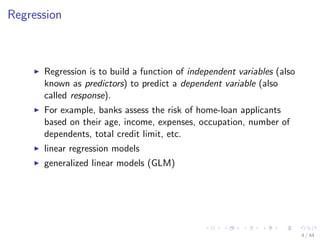
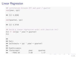
## correlation between CPI and year / quarter
cor(year, cpi)
## [1] 0.9096
cor(quarter, cpi)
## [1] 0.3738
## build a linear regression model with function lm()
fit - lm(cpi ~ year + quarter)
fit
##
## Call:
## lm(formula = cpi ~ year + quarter)
##
## Coefficients:
## (Intercept) year quarter
## -7644.49 3.89 1.17
8 / 44](https://image.slidesharecdn.com/rdatamining-slides-regression-classification-140915032901-phpapp01/85/Regression-and-Classification-with-R-10-320.jpg)
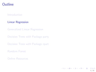
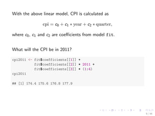
![With the above linear model, CPI is calculated as
cpi = c0 + c1 year + c2 quarter;
where c0, c1 and c2 are coecients from model fit.
What will the CPI be in 2011?
cpi2011 - fit$coefficients[[1]] +
fit$coefficients[[2]] * 2011 +
fit$coefficients[[3]] * (1:4)
cpi2011
## [1] 174.4 175.6 176.8 177.9
9 / 44](https://image.slidesharecdn.com/rdatamining-slides-regression-classification-140915032901-phpapp01/85/Regression-and-Classification-with-R-11-320.jpg)
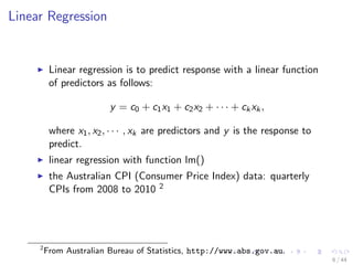
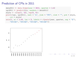
![With the above linear model, CPI is calculated as
cpi = c0 + c1 year + c2 quarter;
where c0, c1 and c2 are coecients from model fit.
What will the CPI be in 2011?
cpi2011 - fit$coefficients[[1]] +
fit$coefficients[[2]] * 2011 +
fit$coefficients[[3]] * (1:4)
cpi2011
## [1] 174.4 175.6 176.8 177.9
An easier way is to use function predict().
9 / 44](https://image.slidesharecdn.com/rdatamining-slides-regression-classification-140915032901-phpapp01/85/Regression-and-Classification-with-R-12-320.jpg)
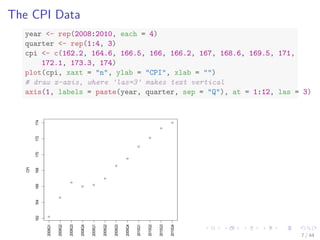
![More details of the model can be obtained with the code below.
attributes(fit)
## $names
## [1] coefficients residuals effects
## [4] rank fitted.values assign
## [7] qr df.residual xlevels
## [10] call terms model
##
## $class
## [1] lm
fit$coefficients
## (Intercept) year quarter
## -7644.488 3.888 1.167
10 / 44](https://image.slidesharecdn.com/rdatamining-slides-regression-classification-140915032901-phpapp01/85/Regression-and-Classification-with-R-13-320.jpg)
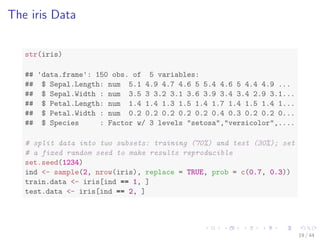
![The iris Data
str(iris)
## 'data.frame': 150 obs. of 5 variables:
## $ Sepal.Length: num 5.1 4.9 4.7 4.6 5 5.4 4.6 5 4.4 4.9 ...
## $ Sepal.Width : num 3.5 3 3.2 3.1 3.6 3.9 3.4 3.4 2.9 3.1...
## $ Petal.Length: num 1.4 1.4 1.3 1.5 1.4 1.7 1.4 1.5 1.4 1...
## $ Petal.Width : num 0.2 0.2 0.2 0.2 0.2 0.4 0.3 0.2 0.2 0...
## $ Species : Factor w/ 3 levels setosa,versicolor,....
# split data into two subsets: training (70%) and test (30%); set
# a fixed random seed to make results reproducible
set.seed(1234)
ind - sample(2, nrow(iris), replace = TRUE, prob = c(0.7, 0.3))
train.data - iris[ind == 1, ]
test.data - iris[ind == 2, ]
19 / 44](https://image.slidesharecdn.com/rdatamining-slides-regression-classification-140915032901-phpapp01/85/Regression-and-Classification-with-R-26-320.jpg)
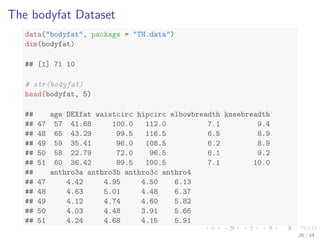
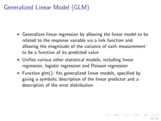
![The bodyfat Dataset
data(bodyfat, package = TH.data)
dim(bodyfat)
## [1] 71 10
# str(bodyfat)
head(bodyfat, 5)
## age DEXfat waistcirc hipcirc elbowbreadth kneebreadth
## 47 57 41.68 100.0 112.0 7.1 9.4
## 48 65 43.29 99.5 116.5 6.5 8.9
## 49 59 35.41 96.0 108.5 6.2 8.9
## 50 58 22.79 72.0 96.5 6.1 9.2
## 51 60 36.42 89.5 100.5 7.1 10.0
## anthro3a anthro3b anthro3c anthro4
## 47 4.42 4.95 4.50 6.13
## 48 4.63 5.01 4.48 6.37
## 49 4.12 4.74 4.60 5.82
## 50 4.03 4.48 3.91 5.66
## 51 4.24 4.68 4.15 5.91
26 / 44](https://image.slidesharecdn.com/rdatamining-slides-regression-classification-140915032901-phpapp01/85/Regression-and-Classification-with-R-33-320.jpg)
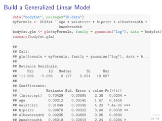
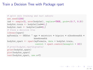
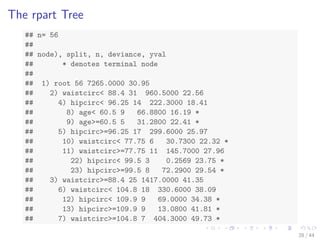
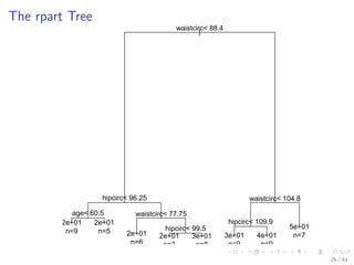
![Train a Decision Tree with Package rpart
# split into training and test subsets
set.seed(1234)
ind - sample(2, nrow(bodyfat), replace=TRUE, prob=c(0.7, 0.3))
bodyfat.train - bodyfat[ind==1,]
bodyfat.test - bodyfat[ind==2,]
# train a decision tree
library(rpart)
myFormula - DEXfat ~ age + waistcirc + hipcirc + elbowbreadth +
kneebreadth
bodyfat_rpart - rpart(myFormula, data = bodyfat.train,
control = rpart.control(minsplit = 10))
# print(bodyfat_rpart$cptable)
print(bodyfat_rpart)
plot(bodyfat_rpart)
text(bodyfat_rpart, use.n=T)
27 / 44](https://image.slidesharecdn.com/rdatamining-slides-regression-classification-140915032901-phpapp01/85/Regression-and-Classification-with-R-34-320.jpg)
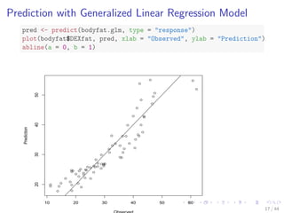
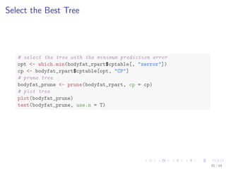
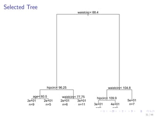
![Select the Best Tree
# select the tree with the minimum prediction error
opt - which.min(bodyfat_rpart$cptable[, xerror])
cp - bodyfat_rpart$cptable[opt, CP]
# prune tree
bodyfat_prune - prune(bodyfat_rpart, cp = cp)
# plot tree
plot(bodyfat_prune)
text(bodyfat_prune, use.n = T)
30 / 44](https://image.slidesharecdn.com/rdatamining-slides-regression-classification-140915032901-phpapp01/85/Regression-and-Classification-with-R-37-320.jpg)
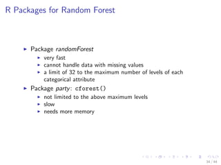
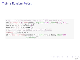
![Train a Random Forest
# split into two subsets: training (70%) and test (30%)
ind - sample(2, nrow(iris), replace=TRUE, prob=c(0.7, 0.3))
train.data - iris[ind==1,]
test.data - iris[ind==2,]
# use all other variables to predict Species
library(randomForest)
rf - randomForest(Species ~ ., data=train.data, ntree=100,
proximity=T)
35 / 44](https://image.slidesharecdn.com/rdatamining-slides-regression-classification-140915032901-phpapp01/85/Regression-and-Classification-with-R-42-320.jpg)


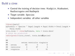
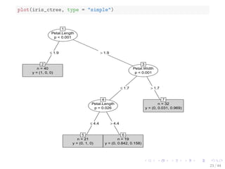
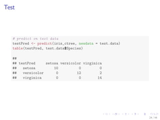
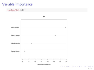
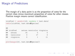
This document discusses building regression and classification models in R, including linear regression, generalized linear models, and decision trees. It provides examples of building each type of model using various R packages and datasets. Linear regression is used to predict CPI data. Generalized linear models and decision trees are built to predict body fat percentage. Decision trees are also built on the iris dataset to classify flower species.


![Introduction to R for Data Science :: Session 6 [Linear Regression in R]](https://cdn.slidesharecdn.com/ss_thumbnails/intrordatasciencesession6eng-160606173046-thumbnail.jpg?width=640&height=640&fit=bounds)


![Getting Started with Apache Spark: Big Data Made Simple [Free Meetup]](https://cdn.slidesharecdn.com/ss_thumbnails/apachesparkgettingstarted-260203175547-8361bcc3-thumbnail.jpg?width=640&height=640&fit=bounds)


