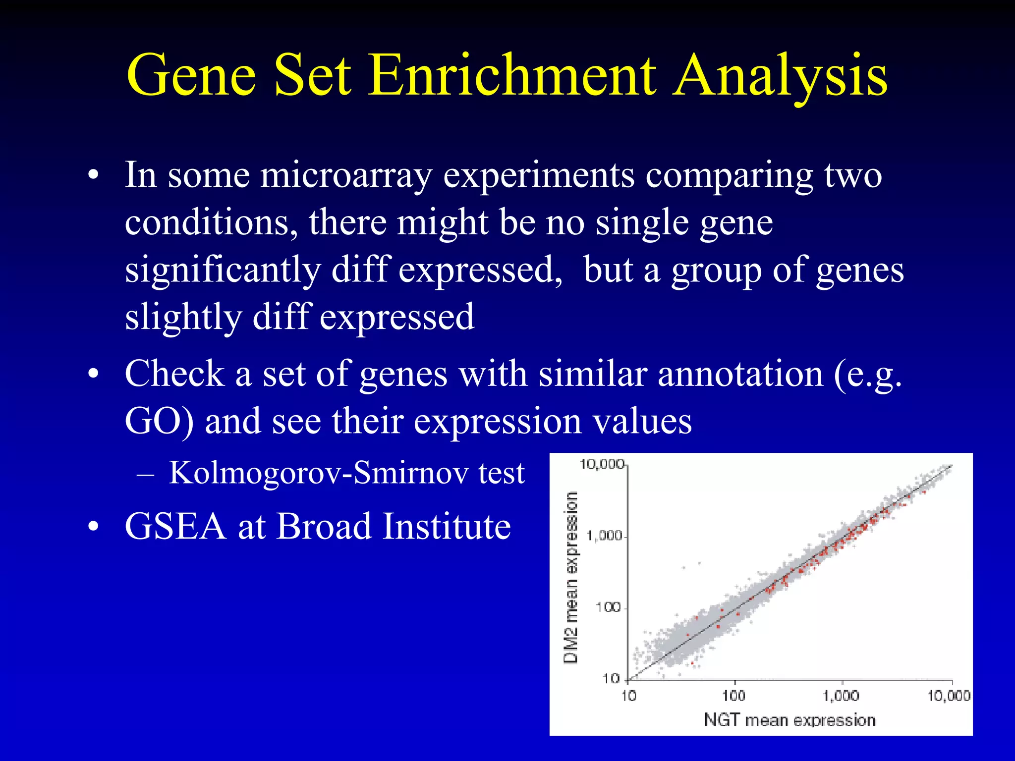
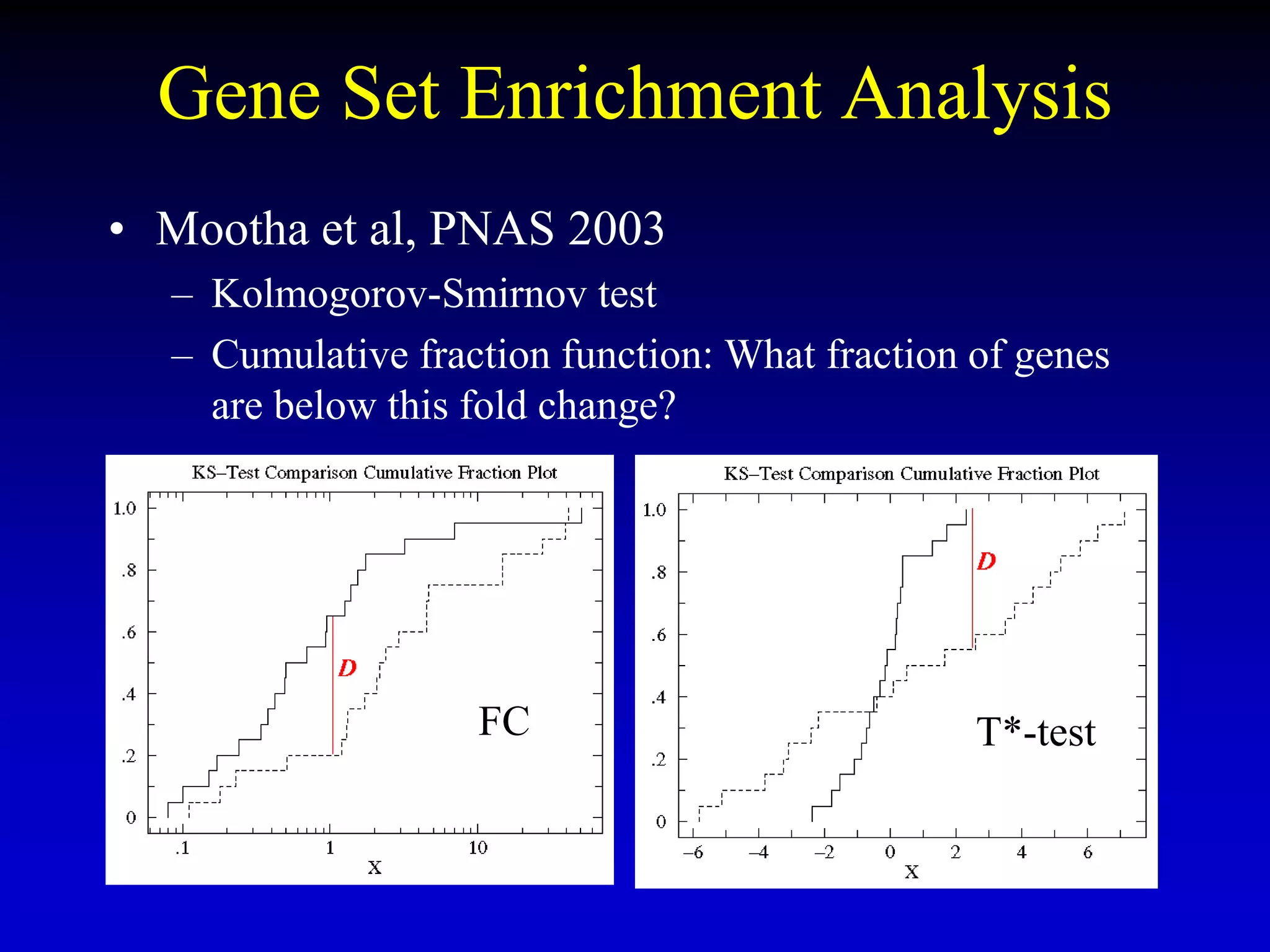
Gene Set Enrichment Analysis
Xiaole Shirley Liu
STAT115/STAT215
Gene Set Enrichment Analysis
• In some microarray experiments comparing two
conditions, there might be no single gene
significantly diff expressed, but a group of genes
slightly diff expressed
• Check a set of genes with similar annotation (e.g.
GO) and see their expression values
– Kolmogorov-Smirnov test
• GSEA at Broad Institute
Gene Set Enrichment Analysis
• Mootha et al, PNAS 2003
– Kolmogorov-Smirnov test
– Cumulative fraction function: What fraction of genes
are below this fold change?
T*-test
FC
STAT115
03/18/2008
4
Gene Set Enrichment Analysis
• Alternative to KS: one sample z-test
– Population with all the genes follow normal ~
N(,2)
– Avg of the genes (X) with a specific
annotation:
|
|
)
(
X
X
z




Gene Set Enrichment Analysis
• Set of genes with specific annotation involved in
coordinated down-regulation
• Need to define the set before looking at the data
• Can only see the significance by looking at the
whole set
Expanded Gene Sets
• Subramanian, et al PNAS 2005
6
Examples of GSEA
7
Break
Microarray Classification
Xiaole Shirley Liu
STAT115/STAT215
9
Microarray Classification
probe set Normal m412a
Normal m414a
Normal m416a
Normal m426a
Normal m430a
MM m282 MM m331a
MM m332a
MM m333a
MM m334a
MM m353a
MM m408a
MM m423a
MM m424a
39089_at 89.31 143.37 111.61 134.78 121.57 104.02 101.11 105.16 121.21 176.72 117.16 137.19 109.5 109.06
35862_at 95.05 107.04 71.06 100.63 117.58 103.96 95.2 114.35 95.03 90.32 93.13 88.61 90.87 112.95
41777_at 22.76 20.05 21.37 25.55 30.8 20.75 21.95 28.82 30.85 28.81 22.65 18.91 22.58 21.65
38250_at 53.55 62.89 29.36 62.74 36.14 60.07 37.46 42.85 27.86 41.48 116.4 46.39 38.9 29.11
656_at 177.69 177.65 167.15 166.04 155.07 180.4 136.47 200.4 201.8 138.38 165.92 176.25 162.85 156.17
332_at 128.5 98.29 130.58 111.49 103.56 115.47 121.01 134.5 118.85 88.71 105.08 93.28 113.18 140.13
39185_at 107.86 114.02 104.08 108.89 112.75 113.61 120.9 120.1 113.82 102.72 109.81 104.86 104.4 95.53
514_at 69.21 51.43 92.43 69.21 55.46 58.43 73.9 74.58 88.07 57.01 79.11 53.63 53.43 69.62
35010_at 65.34 42 48.14 52.85 59.07 49.62 62.59 68.39 55.57 47.92 46.97 49.73 44.7 55.73
34793_s_at 9.95 9.12 10.45 14.65 21.91 13.2 14.02 17.15 9.05 10.66 8.24 13.43 17.17 15.97
33277_at 153.21 120.52 136.7 113.79 110.23 140.96 153.44 149.59 119.14 98.57 156.85 101.86 117.28 104.72
34788_at 167.66 172.86 142.6 199.39 195.34 156.66 173.96 159.16 207.34 154.18 158.59 151.91 171.65 246.11
2053_at 91.76 111.82 99.57 95.58 87.17 123.15 82.24 93.92 97.76 114.66 80.33 107.65 89.78 85.41
33465_at 63.37 45.24 54.72 56.74 58.16 59.55 63.43 71.55 55.76 46.63 49.78 40.49 44.5 69.33
41097_at 145.34 148.08 171.78 151.96 128.26 138.98 148.45 160.25 169.47 133.5 166.24 135.37 159.2 129.96
32394_s_at 449.9 1190.09 429.93 1034.13 196.52 214.51 220.81 331.66 652.66 488.37 699.41 1903.88 843.79 575.16
1969_s_at 30.03 34.58 59.76 32.84 46.98 51.34 40.4 41.75 31.8 36.74 62.42 40.4 36.37 26.06
39225_at 43.19 82.15 97.56 78.3 57.23 65.29 75.14 54.5 58.35 62.47 124.64 56.42 90.55 57.28
36919_r_at 36.45 26.84 37.94 35.79 38.86 33.99 28.94 32.57 39.61 32.08 31.37 36.58 44.33 36.99
33574_at 16.14 12.58 10.93 14.65 29.64 19.38 14.65 15.29 16.14 19.72 11.23 12.6 18.2 24.04
36271_at 41.71 25.8 39.79 49.71 52.64 33.5 48.33 41.15 48.74 45.12 36.5 38.58 55.99 29.73
490_g_at 83.48 103.93 121.57 80.05 73.81 115.47 106.57 96.19 101.49 78.5 86.13 71.87 83.73 93.64
1654_at 78.63 82.7 93.15 73.96 73.82 104.4 100.39 91.78 82.26 63.21 76.23 56.97 76.2 73.04
41207_at 100.27 80.62 84.98 75.44 74.26 95.56 96.83 100.36 85.12 71.34 81.04 75.81 70.77 70.81
40080_at 172.83 106.63 122.03 118.12 131.15 153.53 150.19 161.04 123 101.64 142.03 110.02 113.58 117.18
38699_at 69.1 67.16 62.73 67.46 74.03 61.16 75.27 75.7 63.2 68.12 57.25 65.42 70.71 75.81
698_f_at 21.36 43.88 30.5 65.43 35.73 44.05 32.34 35.17 33.89 62.61 34.72 42.49 32.13 37.51
36036_at 105.59 71.45 88.72 79.84 75.78 95.13 115.07 100.81 84.13 69.87 76.51 71.58 72.16 73.85
40720_at 104.84 175.9 186.87 65.58 64 204.55 89.48 110.87 99 59.84 138.3 59.43 197.43 118.32
32194_at 34.01 165.32 153.91 59.4 43.4 98.5 59.53 43.28 47.98 63.09 217.29 127.38 79.38 82.04
31499_s_at 42.66 36.26 47.61 43.35 48.55 40.87 52.57 53.86 41.41 40.08 44.22 35.6 43.32 41.48
41685_at 25.07 14.68 22.41 22.98 19.79 22.21 21.85 25.12 20.27 18.44 20.37 12.85 22.02 25.91
31788_at 115.87 151.38 103.33 144.45 138.01 125.9 132.74 121.06 113.56 114.21 149.88 199.76 121.17 96.03
1719_at 15.65 18.26 16.74 21.49 15.16 11.49 17.52 21.35 19.36 20.6 15.13 14.3 18.77 18.49
973_at 169.15 142.44 164.57 129 151.38 189.15 171.12 169.57 139.02 140.37 145.62 145.17 130.23 132.35
?
10
Classification
• Equivalent to machine learning methods
• Task: assign object to class based on
measurements on object
– E.g. is sample normal or cancer based on expression
profile?
• Unsupervised learning
– Ignore known class labels
– Sometimes can’t separate even the known classes
• Supervised learning:
– Extract useful features based on known class labels to
best separate classes
– Can over fit the data, so need to separate training and
test set
11
Clustering Classification
• Which known samples does the unknown sample
cluster with?
• No guarantee that the known sample will cluster
• Try batch removal or different clustering methods
– Change linkage, select subset genes (semi-supervised)
12
K Nearest Neighbor
• Used in missing value estimation
• For observation X with unknown label, find
the K observations in the training data
closest (e.g. correlation) to X
• Predict the label of X based on majority
vote by KNN
• K can be determined by predictability of
known samples, semi-supervised again!
KNN Example
• Can extend KNN by
assigning weights to the
neighbors by inverse
distance from the test-
sample
• Offer little insights into
mechanism
13
14
MDS
• Multidimensional scaling
• Based on distance between data in high
dimensional space (e.g. correlations)
• Give 2-3D representation approximating the
pairwise distance relationship as much as
possible
• Non-linear projection
• Can directly predict
new sample based on dist
Break
15
Principal Component Analysis
• Linear transformation that projects the data on to new
coordinate system (linear combinations of the original
variables) to capture as much of the variation in data as
possible
• The first principal component accounts for the greatest
possible variance in dataset
• The second principal component accounts for the next
highest variance and is uncorrelated with (orthogonal to)
the first principal component.
Finding the Projections
• Looking for a linear combination to transform the
original data matrix X to:
Y= T X=1 X1+ 2 X2+..+ p Xp
• Where  =(1 , 2 ,.., p)T is a column vector of
weights with
1²+ 2²+..+ p² =1
• Maximize the variance of the projection of the
observations on the Y variables
Finding the Projections
• The direction of  is given by the eigenvector 1
correponding to the largest eigenvalue of matrix C
• The second vector that is orthogonal (uncorrelated) to the
first is the one that has the second highest variance which
comes to be the eignevector corresponding to the second
eigenvalue
17
Good Better
18
Principal Component Analysis
• Achieved by singular value decomposition (SVD):
X = UDVT
• X is the original data
• U (N × N) is the relative
projection of the points
• V is project directions
– v1 is a unit vector, direction of the first projection
– The eigenvector with the largest eigenvalue
– Linear combination (relative importance) of each gene
(if PCA on samples)
19
PCA
• D is scaling factor (eigenvalue)
– Diagonal matrix, d1  d2  d3  …  0
– dm
2 measures the variances captures by the mth principal
component
• u1d1 is distance along v1 from origin (first
principal components)
– Expression value projected on v1
– u1d1 captures the largest variance of original X
– v2 is 2nd projection direction, orthogonal to PC1, u2d2 is
2nd principal component and captures the 2nd largest var
of X
PCA for Classification
20
Blood transcriptome of
healthy individual (HI),
cardiovascular risk factor
individuals (RF),
individuals with
asymptomatic left
ventricular dysfunction
groups (ALVD) and
chronic heart failure
patients (CHF).
New sample predicted to
be CHF.
Interpretation of components
• See the weights of variables in each component
• If Y1= 0.41X1 +0.15X2 -0.38X3+0.03X4+…
• X1 and X3 are more important than X2 and X4 in PC1,
offers some biological insights
• PCA and MDS are both good dimension reduction
methods
• PCA is a good clustering method, and can be conducted
on genes or on samples
• PCA is only powerful if the biological question is
related to the highest variance in the dataset
PCA for Batch Effect Detection
• PCA can identify batch effect
• Obvious batch effect: early PC’s separate
samples by batch
22
Un-normalized Qnorm COMBAT
Brezina et al, Microarray 2015
Break
Supervised Learning
23
24
Supervised Learning
Performance Assessment
• If error rate is estimated from whole learning data
set, could overfit the data (do well now, but poorly
in future observations)
• Need cross validation to assess performance
• Leave-1 cross validation on n data points
– Build classifier on (n-1), test on the one left out
• N-fold cross validation
– Divide data into N subset (equal size), build classifier
on (N-1) subsets, compute error rate on left out subset
26
Logistic Regression
• Data: (yi, xi), i=1,…, n
• Dependent variable is binary: 0, 1
• Model
• Logit: natural log of odds ratio Pb(1) over Pb(0)
• b0+b1X really big, Y =1; b0+b1X really small, Y =0
• But change in probability is not linear with changes in X
• b0  intercept
• b1  regression slope
• b0+b1X = 0  decision
boundary Pb(1) = 0.5
0 1 1
ˆ
( 1| )
exp( )
ˆ
(1 ( 1| )) (1 )
i
i
i
P Y X
b b X
P Y X


   

  
   
  
 
 
Example (wiki)
• Hours study on Pb of passing an exam
• Significant association
– P-value 0.0167
• Pb (pass) = 1/[1+exp(-b0-b1X)]
= 1/[1+exp(4.0777-1.5046* Hours)]
• 4.0777/1.5046 = 2.71 hours  Pb (pass) = 0.5
27
28
Logistic Regression
• Sample classification: Y  Cancer 1, Normal 0
• Find subset of p genes whose expression x
collectively predict new sample classification
• ’s are estimated from training data (R)
• The decision boundary is determined by the linear
regression, i.e., classify yi =1 if:
• More later in the semester
ip
p
i
i
i
i
i
x
x
y
P
y
P


 






1
1
0
)
|
0
(
)
|
1
(
log
x
x
29
Support Vector Machine
• SVM
– Which hyperplane is the best?
30
Support Vector Machine
• SVM finds the hyperplane that maximizes
the margin
• Margin determined by support vectors
(samples lie on the class
edge), others irrelevant
31
Support Vector Machine
• SVM finds the hyperplane that maximizes
the margin
• Margin determined by support vectors
others irrelevant
• Extensions:
– Soft edge, support vectors diff
weight
– Non separable: slack var  > 0
Max (margin –   # bad)
Nonlinear SVM
• Project the data through higher dimensional space
with kernel function, so classes can be separated
by hyperplane
• A few implemented kernel functions available in
BioConductor, the choice is usually trial and error
and personal experience
K(x,y) = (xy)2
33
Outline
• GSEA for activities of group of genes
• Dimension reduction techniques
– MDS, PCA
• Unsupervised learning method
– Clustering, KNN, MDS
– PCA, batch effect
• Supervised learning for classification
– Logistic regression
– SVM
– Cross validation

Lect5_GSEA_Classify (1).ppt

  • 1.
    Gene Set EnrichmentAnalysis Xiaole Shirley Liu STAT115/STAT215
  • 2.
    Gene Set EnrichmentAnalysis • In some microarray experiments comparing two conditions, there might be no single gene significantly diff expressed, but a group of genes slightly diff expressed • Check a set of genes with similar annotation (e.g. GO) and see their expression values – Kolmogorov-Smirnov test • GSEA at Broad Institute
  • 3.
    Gene Set EnrichmentAnalysis • Mootha et al, PNAS 2003 – Kolmogorov-Smirnov test – Cumulative fraction function: What fraction of genes are below this fold change? T*-test FC
  • 4.
    STAT115 03/18/2008 4 Gene Set EnrichmentAnalysis • Alternative to KS: one sample z-test – Population with all the genes follow normal ~ N(,2) – Avg of the genes (X) with a specific annotation: | | ) ( X X z    
  • 5.
    Gene Set EnrichmentAnalysis • Set of genes with specific annotation involved in coordinated down-regulation • Need to define the set before looking at the data • Can only see the significance by looking at the whole set
  • 6.
    Expanded Gene Sets •Subramanian, et al PNAS 2005 6
  • 7.
  • 8.
  • 9.
    9 Microarray Classification probe setNormal m412a Normal m414a Normal m416a Normal m426a Normal m430a MM m282 MM m331a MM m332a MM m333a MM m334a MM m353a MM m408a MM m423a MM m424a 39089_at 89.31 143.37 111.61 134.78 121.57 104.02 101.11 105.16 121.21 176.72 117.16 137.19 109.5 109.06 35862_at 95.05 107.04 71.06 100.63 117.58 103.96 95.2 114.35 95.03 90.32 93.13 88.61 90.87 112.95 41777_at 22.76 20.05 21.37 25.55 30.8 20.75 21.95 28.82 30.85 28.81 22.65 18.91 22.58 21.65 38250_at 53.55 62.89 29.36 62.74 36.14 60.07 37.46 42.85 27.86 41.48 116.4 46.39 38.9 29.11 656_at 177.69 177.65 167.15 166.04 155.07 180.4 136.47 200.4 201.8 138.38 165.92 176.25 162.85 156.17 332_at 128.5 98.29 130.58 111.49 103.56 115.47 121.01 134.5 118.85 88.71 105.08 93.28 113.18 140.13 39185_at 107.86 114.02 104.08 108.89 112.75 113.61 120.9 120.1 113.82 102.72 109.81 104.86 104.4 95.53 514_at 69.21 51.43 92.43 69.21 55.46 58.43 73.9 74.58 88.07 57.01 79.11 53.63 53.43 69.62 35010_at 65.34 42 48.14 52.85 59.07 49.62 62.59 68.39 55.57 47.92 46.97 49.73 44.7 55.73 34793_s_at 9.95 9.12 10.45 14.65 21.91 13.2 14.02 17.15 9.05 10.66 8.24 13.43 17.17 15.97 33277_at 153.21 120.52 136.7 113.79 110.23 140.96 153.44 149.59 119.14 98.57 156.85 101.86 117.28 104.72 34788_at 167.66 172.86 142.6 199.39 195.34 156.66 173.96 159.16 207.34 154.18 158.59 151.91 171.65 246.11 2053_at 91.76 111.82 99.57 95.58 87.17 123.15 82.24 93.92 97.76 114.66 80.33 107.65 89.78 85.41 33465_at 63.37 45.24 54.72 56.74 58.16 59.55 63.43 71.55 55.76 46.63 49.78 40.49 44.5 69.33 41097_at 145.34 148.08 171.78 151.96 128.26 138.98 148.45 160.25 169.47 133.5 166.24 135.37 159.2 129.96 32394_s_at 449.9 1190.09 429.93 1034.13 196.52 214.51 220.81 331.66 652.66 488.37 699.41 1903.88 843.79 575.16 1969_s_at 30.03 34.58 59.76 32.84 46.98 51.34 40.4 41.75 31.8 36.74 62.42 40.4 36.37 26.06 39225_at 43.19 82.15 97.56 78.3 57.23 65.29 75.14 54.5 58.35 62.47 124.64 56.42 90.55 57.28 36919_r_at 36.45 26.84 37.94 35.79 38.86 33.99 28.94 32.57 39.61 32.08 31.37 36.58 44.33 36.99 33574_at 16.14 12.58 10.93 14.65 29.64 19.38 14.65 15.29 16.14 19.72 11.23 12.6 18.2 24.04 36271_at 41.71 25.8 39.79 49.71 52.64 33.5 48.33 41.15 48.74 45.12 36.5 38.58 55.99 29.73 490_g_at 83.48 103.93 121.57 80.05 73.81 115.47 106.57 96.19 101.49 78.5 86.13 71.87 83.73 93.64 1654_at 78.63 82.7 93.15 73.96 73.82 104.4 100.39 91.78 82.26 63.21 76.23 56.97 76.2 73.04 41207_at 100.27 80.62 84.98 75.44 74.26 95.56 96.83 100.36 85.12 71.34 81.04 75.81 70.77 70.81 40080_at 172.83 106.63 122.03 118.12 131.15 153.53 150.19 161.04 123 101.64 142.03 110.02 113.58 117.18 38699_at 69.1 67.16 62.73 67.46 74.03 61.16 75.27 75.7 63.2 68.12 57.25 65.42 70.71 75.81 698_f_at 21.36 43.88 30.5 65.43 35.73 44.05 32.34 35.17 33.89 62.61 34.72 42.49 32.13 37.51 36036_at 105.59 71.45 88.72 79.84 75.78 95.13 115.07 100.81 84.13 69.87 76.51 71.58 72.16 73.85 40720_at 104.84 175.9 186.87 65.58 64 204.55 89.48 110.87 99 59.84 138.3 59.43 197.43 118.32 32194_at 34.01 165.32 153.91 59.4 43.4 98.5 59.53 43.28 47.98 63.09 217.29 127.38 79.38 82.04 31499_s_at 42.66 36.26 47.61 43.35 48.55 40.87 52.57 53.86 41.41 40.08 44.22 35.6 43.32 41.48 41685_at 25.07 14.68 22.41 22.98 19.79 22.21 21.85 25.12 20.27 18.44 20.37 12.85 22.02 25.91 31788_at 115.87 151.38 103.33 144.45 138.01 125.9 132.74 121.06 113.56 114.21 149.88 199.76 121.17 96.03 1719_at 15.65 18.26 16.74 21.49 15.16 11.49 17.52 21.35 19.36 20.6 15.13 14.3 18.77 18.49 973_at 169.15 142.44 164.57 129 151.38 189.15 171.12 169.57 139.02 140.37 145.62 145.17 130.23 132.35 ?
  • 10.
    10 Classification • Equivalent tomachine learning methods • Task: assign object to class based on measurements on object – E.g. is sample normal or cancer based on expression profile? • Unsupervised learning – Ignore known class labels – Sometimes can’t separate even the known classes • Supervised learning: – Extract useful features based on known class labels to best separate classes – Can over fit the data, so need to separate training and test set
  • 11.
    11 Clustering Classification • Whichknown samples does the unknown sample cluster with? • No guarantee that the known sample will cluster • Try batch removal or different clustering methods – Change linkage, select subset genes (semi-supervised)
  • 12.
    12 K Nearest Neighbor •Used in missing value estimation • For observation X with unknown label, find the K observations in the training data closest (e.g. correlation) to X • Predict the label of X based on majority vote by KNN • K can be determined by predictability of known samples, semi-supervised again!
  • 13.
    KNN Example • Canextend KNN by assigning weights to the neighbors by inverse distance from the test- sample • Offer little insights into mechanism 13
  • 14.
    14 MDS • Multidimensional scaling •Based on distance between data in high dimensional space (e.g. correlations) • Give 2-3D representation approximating the pairwise distance relationship as much as possible • Non-linear projection • Can directly predict new sample based on dist Break
  • 15.
    15 Principal Component Analysis •Linear transformation that projects the data on to new coordinate system (linear combinations of the original variables) to capture as much of the variation in data as possible • The first principal component accounts for the greatest possible variance in dataset • The second principal component accounts for the next highest variance and is uncorrelated with (orthogonal to) the first principal component.
  • 16.
    Finding the Projections •Looking for a linear combination to transform the original data matrix X to: Y= T X=1 X1+ 2 X2+..+ p Xp • Where  =(1 , 2 ,.., p)T is a column vector of weights with 1²+ 2²+..+ p² =1 • Maximize the variance of the projection of the observations on the Y variables
  • 17.
    Finding the Projections •The direction of  is given by the eigenvector 1 correponding to the largest eigenvalue of matrix C • The second vector that is orthogonal (uncorrelated) to the first is the one that has the second highest variance which comes to be the eignevector corresponding to the second eigenvalue 17 Good Better
  • 18.
    18 Principal Component Analysis •Achieved by singular value decomposition (SVD): X = UDVT • X is the original data • U (N × N) is the relative projection of the points • V is project directions – v1 is a unit vector, direction of the first projection – The eigenvector with the largest eigenvalue – Linear combination (relative importance) of each gene (if PCA on samples)
  • 19.
    19 PCA • D isscaling factor (eigenvalue) – Diagonal matrix, d1  d2  d3  …  0 – dm 2 measures the variances captures by the mth principal component • u1d1 is distance along v1 from origin (first principal components) – Expression value projected on v1 – u1d1 captures the largest variance of original X – v2 is 2nd projection direction, orthogonal to PC1, u2d2 is 2nd principal component and captures the 2nd largest var of X
  • 20.
    PCA for Classification 20 Bloodtranscriptome of healthy individual (HI), cardiovascular risk factor individuals (RF), individuals with asymptomatic left ventricular dysfunction groups (ALVD) and chronic heart failure patients (CHF). New sample predicted to be CHF.
  • 21.
    Interpretation of components •See the weights of variables in each component • If Y1= 0.41X1 +0.15X2 -0.38X3+0.03X4+… • X1 and X3 are more important than X2 and X4 in PC1, offers some biological insights • PCA and MDS are both good dimension reduction methods • PCA is a good clustering method, and can be conducted on genes or on samples • PCA is only powerful if the biological question is related to the highest variance in the dataset
  • 22.
    PCA for BatchEffect Detection • PCA can identify batch effect • Obvious batch effect: early PC’s separate samples by batch 22 Un-normalized Qnorm COMBAT Brezina et al, Microarray 2015 Break
  • 23.
  • 24.
    24 Supervised Learning Performance Assessment •If error rate is estimated from whole learning data set, could overfit the data (do well now, but poorly in future observations) • Need cross validation to assess performance • Leave-1 cross validation on n data points – Build classifier on (n-1), test on the one left out • N-fold cross validation – Divide data into N subset (equal size), build classifier on (N-1) subsets, compute error rate on left out subset
  • 25.
    26 Logistic Regression • Data:(yi, xi), i=1,…, n • Dependent variable is binary: 0, 1 • Model • Logit: natural log of odds ratio Pb(1) over Pb(0) • b0+b1X really big, Y =1; b0+b1X really small, Y =0 • But change in probability is not linear with changes in X • b0  intercept • b1  regression slope • b0+b1X = 0  decision boundary Pb(1) = 0.5 0 1 1 ˆ ( 1| ) exp( ) ˆ (1 ( 1| )) (1 ) i i i P Y X b b X P Y X                     
  • 26.
    Example (wiki) • Hoursstudy on Pb of passing an exam • Significant association – P-value 0.0167 • Pb (pass) = 1/[1+exp(-b0-b1X)] = 1/[1+exp(4.0777-1.5046* Hours)] • 4.0777/1.5046 = 2.71 hours  Pb (pass) = 0.5 27
  • 27.
    28 Logistic Regression • Sampleclassification: Y  Cancer 1, Normal 0 • Find subset of p genes whose expression x collectively predict new sample classification • ’s are estimated from training data (R) • The decision boundary is determined by the linear regression, i.e., classify yi =1 if: • More later in the semester ip p i i i i i x x y P y P           1 1 0 ) | 0 ( ) | 1 ( log x x
  • 28.
    29 Support Vector Machine •SVM – Which hyperplane is the best?
  • 29.
    30 Support Vector Machine •SVM finds the hyperplane that maximizes the margin • Margin determined by support vectors (samples lie on the class edge), others irrelevant
  • 30.
    31 Support Vector Machine •SVM finds the hyperplane that maximizes the margin • Margin determined by support vectors others irrelevant • Extensions: – Soft edge, support vectors diff weight – Non separable: slack var  > 0 Max (margin –   # bad)
  • 31.
    Nonlinear SVM • Projectthe data through higher dimensional space with kernel function, so classes can be separated by hyperplane • A few implemented kernel functions available in BioConductor, the choice is usually trial and error and personal experience K(x,y) = (xy)2
  • 32.
    33 Outline • GSEA foractivities of group of genes • Dimension reduction techniques – MDS, PCA • Unsupervised learning method – Clustering, KNN, MDS – PCA, batch effect • Supervised learning for classification – Logistic regression – SVM – Cross validation