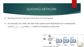
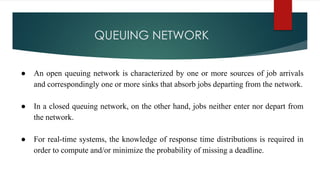
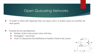
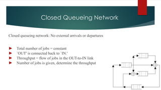
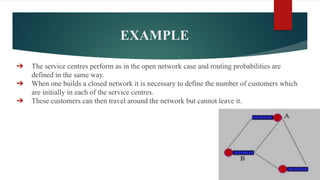
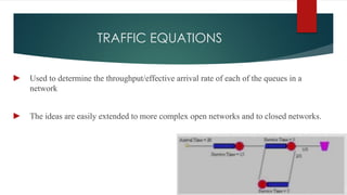
This document discusses queueing networks and probability models. It defines queueing networks as interconnected queues and describes open, closed, and mixed queueing networks. Open networks have external arrivals and departures, while closed networks have a fixed number of jobs. Mixed networks can be open for some workloads and closed for others. The document provides examples of different network types and discusses properties like jockeying. It also covers traffic equations used to determine throughput and mean value analysis for solving closed networks.

1. QUEUING
NETWORKS
PROBABILITY MODELS

2. INTRODUCTION
Queueing theory is the mathematical study of waiting lines, or queues.
A queueing model is constructed so that queue lengths and waiting time can be predicted.
In a model for computer system performance analysis, we may have a service center for the
CPU(s), a service center for each I/O channel, and possibly others.

3. QUEUING NETWORK
● Queuing network is the inter connections of several queues.
● For networks of m nodes, the state of the system can be described by an m–dimensional
vector (x1
, x2
, ..., xm
) where xi
= number of customers at each node.

4. QUEUING NETWORK
● An open queuing network is characterized by one or more sources of job arrivals
and correspondingly one or more sinks that absorb jobs departing from the network.
● In a closed queuing network, on the other hand, jobs neither enter nor depart from
the network.
● For real-time systems, the knowledge of response time distributions is required in
order to compute and/or minimize the probability of missing a deadline.

5. EXAMPLE
● Customers go from one queue to another in post office, bank, supermarket etc.
● Data packets traverse a network moving from a queue in a router to the queue in another router

6. CLASSIFICATION
► OPEN QUEUING NETWORK
► CLOSE QUEUING NETWORK
► MIXED QUEUING NETWORK

7. Open Queueing Networks
► A model in which jobs departing from one queue arrive at another queue (or possibly the
same queue)
► External arrivals and departures.
● Number of jobs in the system varies with time.
● Throughput = arrival rate.
● Goal: To characterize the distribution of number of jobs in the system.

8. EXAMPLE
➔ The yellow circle B, represents an external source of customers.
➔ Three inter-connected service centres and an external destination C.
➔ Attaching a weighting to each possible destination.
➔ For example customer leaving queue 2, there are 2 possible destinations.
➔ However, if queue1 had weight 1 and queue 0 had weight 2, then , on average, 1 in 3 customers
would go to queue 1 and 2 in 3 customers would go to queue 0.

9. Closed Queueing Network
Closed queueing network: No external arrivals or departures
► Total number of jobs = constant
► `OUT' is connected back to `IN.'
► Throughput = flow of jobs in the OUT-to-IN link
► Number of jobs is given, determine the throughput

10. EXAMPLE
➔ The service centres perform as in the open network case and routing probabilities are
defined in the same way.
➔ When one builds a closed network it is necessary to define the number of customers which
are initially in each of the service centres.
➔ These customers can then travel around the network but cannot leave it.

11. Mixed Queueing Network
► Open for some workloads and closed for others ⇒ Two classes of jobs.
► All jobs of a single class have the same service demands and transition probabilities.
Within each class, the jobs are indistinguishable.

12. EXAMPLE
► simple model of virtual circuit that is window flow controlled.

13. PROPERTIES
► Jockeying
► Blocking
► Routing
► Forking
► Joining

14. TRAFFIC EQUATIONS
► Used to determine the throughput/effective arrival rate of each of the queues in a
network
► The ideas are easily extended to more complex open networks and to closed networks.

15. TRAFFIC EQUATIONS
➔ We consider each queue in turn
➔ Queue 0 : Input to queue is 0
◆ The arrival rate from the source i.e 1/20.
◆ So the first traffic equation is: Xo = 1/20.
➔ Queue 1:
◆ X1=Xo+X2
➔ Queue 2: It only gets ⅔ of the customers that leave queue 1
◆ X2 = ⅔ X1
➔ For this example we get : Xo = 0.05 , X1= 0.15 , X2 = 0.1

16. MEAN VALUE ANALYSIS
❏ This allows solving closed queueing networks in a manner similar to that used for open
queueing networks.
❏ It gives the mean performance.
❏ Given a closed queueing network with N jobs: Ri(N) = Si (1+Qi(N-1))
❏ Here, Qi(N-1) is the mean queue length at ith device with N-1 jobs in the network

17. MEAN VALUE ANALYSIS
► Performance with no users ( N=0 ) can be easily computed
► Given the response times at individual devices, the system response time using the general response time
law is:

18. Jackson’s Theorem
► Jackson’s Theorem states that provided the arrival rate at each queue is such that equilibrium exists,
the probability of the overall system state (n1…….nK ) for K queues will be given by the product
form expression

19. Jackson’s Theorem Attributes
In Jackson”s network:
► Only one servers (M/M/1)
► queue disciplines “FCFS”
► Infinite waiting capacity
► Poisson input
► Open networks

20. THANK YOU