Unit-IV; Professional Sales Representative (PSR).pptx
Queueing theory
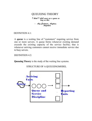
1. QUEUEING THEORY
I think I shall never see a queue as
long as this.
- Any Customer, Anytime,
Anywhere
DEFINITION 4.1:
A queue is a waiting line of "customers" requiring service from
one or more servers. A queue forms whenever existing demand
exceeds the existing capacity of the service facility; that is
whenever arriving customers cannot receive immediate service due
to busy servers.
DEFINITION 4.2:
Queueing Theory is the study of the waiting line systems.
STRUCTURE OF A QUEUEINGMODEL
2. I. COMPONENTS OF THE QUEUEING PROCESS
1.0. The Arrival Process
A. The calling source may be single or multiple populations.
B. The calling source may be finite or infinite.
C. Single or bulk arrivals may occur.
D. Total, partial or no control of arrivals can be exercised by the
queueing system.
E. Units can emanate from a deterministic or probabilistic
generating process.
F. A probabilistic arrival process can be described either by an
empirical or a theoretical probability distribution.
G. A stationary arrival process may or may not exist.
2.0 The Queue Configuration
The queue configuration refers to the number of queues in the
system, their relationship to the servers and spatial consideration.
A. A queue may be a single queue or a multiple queue.
B. Queues may exist
B.1 physically in one place
B.2 physically in disparate locations
B.3 conceptually
B.4 not at all
C. A queueing system may impose restriction on the maximum
number of units allowed.
3. 3.0 Queue Discipline
The following disciplines are possible:
A. lf the system is filled to capacity, the arriving unit is rejected
B. Balking - a customer does not join the queue
C. Reneging - a customer joins the queue and subsequently
decides to leave
D. Collusion - customers collaborate to reduce waiting time
E. Jockeying - a customer switching between multiple queues
F. Cycling - a customer returning to the queue after being given
service
Customers who do not balk, renege, collude, jockey,
cycle, nonrandomly select from among multiple queues
are said to be patient.
4.0 Service Discipline
A. First-Come, First-Served (FCFS)
B. Last-Come, First-Served (LCFS)
C. Service in Random Order (SIRO)
D. Round Robin Service
E. Priority Service
. preemptive
. non-preemptive
4. 5.0. Service Facility
A. The service facility can have none, one, or multiple servers.
B. Multiple servers can be parallel, in series (tandem) or both.
Single Queue, Single Server
..
..
Multiple Queue, Multiple Servers
..
Single Queue, Multiple Servers
5. Multiple Servers in Series
Multiple Servers, both in series and parallel
Channels in parallel may be cooperative or
uncooperative. By policy, channels can also be variable.
C. Service times can be deterministic or probabilistic. Random
variables may be specified by an empirical or theoretical
distribution.
D. State: Dependent state parameters refer to cases where the
parameters refer to cases where the parameters are affected by
a change of the number of units in the system.
E. Breakdowns among servers can also be considered.
6.
7. CLASSIFICATIONS OF MODELS AND SOLUTIONS
1.0. Taxonomy of Queueing Models
A model may be represented using the Kendall- Lee
Notation:
(a/b/c):( d/e/f)
where:
a = arrival rate distribution
b = service rate distribution
c = no. of parallel service channels (identical
service)
d = service discipline
e = maximum no. allowed in the system
f = calling source
Common Notations:
M – Poissonl/Exponential rates
G - General Distribution of Service Times
Ek - Erlangian Distribution
2.0 Methods of Solution
A. Analytical: The use of standard queueing models yields
analytical results.
B. Simulation: Some complex queueing systems cannot be
solved analytically. (non-Poisson models)
8. 3.0 Transient vs. Steady State
A. A solution in the transient state is one that is time
dependent.
B. A solution is in the steady state when it is in statistical
equilibrium (time independent)
4.0 Analytical Queueing Models - Information Flow
In steady state systems, the operating characteristics do not
vary with time.
Notations
λc = effective mean arrival rate
λ = λc if queue is infinite
λe = λ - [expected number who balk if the queue is finite]
W = expected waiting time of a customer in the system
Wq = expected waiting time of a customer in the queue
L = expected no. of customers in the system
Lq = expected number of customers in the queue
Po = probability of no customers in the system
Pn = probability of n customers in the system
ρ = traffic intensity= λ/μ
ρc = effective traffic intensity= λe/μ
9.
10. GENERAL RELATIONSHIPS: (LITTLE'S FORMULA)
The following expressions are valid for all queueing models.These
relationships were developed by J. Little
L=λW
Lq = λWq
W =Wq+1/μ
L = L q + λ/ μ
Note: lf the queue is finite, λ is replaced by λe
EXPONENTIAL QUEUEING MODELS
In the models that will be presented the following assumptions hold
true for any model:
1. The customers of the queueing system are patient customers.
2. The service discipline is general discipline (GD), which means
that the derivations do not consider any specific type of service
discipline.
The derivation of the queueing models involve the use of a set of
difference-differential equations which allow the determination of
the state probabilities. These state probabilities can also be
calculated by the use of the following principle:
Rate-Equality Principle: The rate at which the process enters state n
equals the rate at which it leaves state n.
11. CASE 1: SINGLE CHANNEL-POISSON/EXPONENTIAL
MODEL [(M/M/1):(GD/ α /α)]
Characteristics:
1. Input population is infinite.
2. Arrival rate has a Poisson Distribution
3. There is only one server.
4. Service time is exponentially distributed with mean 1/μ. [λ<μ]
5. System capacity is infinite. .
6. Balking and reneging are not allowed.
Using the rate-equality principle, we obtain our first equation for this
type of system:
λPo=μP1
To understand the above relationship, consider state 0. When in
state 0, the process can leave this state only by an arrival. Since the
arrival rate is λ and the proportion of the time that the process is in
state 0 is given by Po, it follows that the rate at which the process
leaves state 0 is λPo. On the other hand, state 0 can only be reached
from state 1 via a departure. That is, if there is a single customer in
the system and he completes service, then the system becomes
empty. Since the service rate is μ and the proportion of the time that
the system has exactly once customer is P1, it follows that the rate
at which the process enters 0 is μPl. The balance equations using
this principle for any n can now be written as:
State Rate at which the process leaves = rate at which it enters
0 λ P0=μP1
.
12. n ≥1 (λ + μ)Pn = λP + μP
n-1 n+l
In order to solve the above equations, we rewrite them to
obtain
Solving in terms of P0
yields:
In order to determine P0, we use the fact that the Pn must
sum to 1, and thus
or
13. Note that for the above equations to be valid, it is necessary for
to be less than 1 so that the sun of the geometric progression
customers in the system at any time, we use
The last equation follows upon application of the algebraic identity
The rest of the steady state queueing statistics can be calculated
using the expression for L and Little's Formula. A summary of
the queueing formulas for Case I is given below.
14. SUMMARY OF CASE 1 FORMULAS
CASE II : MULTIPLE SERVER, POISSON/
15. EXPONENTIAL MODEL [(M/M/C):(GD/∞/∞ )]
The assumptions of Case II are the same as Case 1 except that
the number of service channels is more than one. For this case, the
service rate of the system is given by:
cµ η≥ c
ηµ η<c
Thus, a multiple server model is equivalent to a single-server
system with service rate varying with η.
λη = λ & µη = ηµ η < c
Using the equality rate principle we have the following balance
equations:
=0
20. CASE III: SINGLE CHANNEL.POISSON ARRIVALS,
ARBITRARY SERVICE TIME: Pollaczek - Khintchine Formula
[(M/G/l): (GD/∞/∞)]
This case is similar to Case 1 except that the service rate
distribution is arbitrary.
Let:
N = no. of units in the queueing system immediately after a unit
departs
T = the time needed to service the unit that follows the one
departing (unit 1) at the beginning of the time count.
K= no. of new arrivals units the system during the time needed to
service the unit that follows the one departing (unit 1)
Nl = no. of units left in the system when the unit (1) departs
Then:
Nl = N + K – 1; if N = 0
=K
Let:
a = 1 if N = 0
a = 0 if N > 0 a*N =0
Then:
Nl = N + K + a – 1
In a steady state system: ~.
E(N)= E( )
E( )= E[ ]
E( )=
21. E (a) = -E (K) + 1
=
=
Since a = 0 or 1: a*N= 0
But
Therefore :
but E(a) = 1 - E(K)
Then:
22. If the arrival rate is Poisson ,
E(K/t) = λt
But in a Poisson Distribution: Mean = Variance
E (K2/t) = λt + (λt)2
23. Substituting and solving for E(N):
The other quantities can be solved using the general relationships
derived by Little.
25. CASE IV: POISSON ARRIVAL AND SERVICE RATE,
INFINITE NUMBER OF SERVERS: Self-Service Model
[(M/M/∞): (GD/∞/∞)]
Consider a multiple server system. The equivalent single server
system if the number of servers is infinite would be:
From the multiple server system:
But
26. Therefore:
Since the number of servers is infinite: Lq = Wq = 0.
Solving for L:
Again, W could be solved using Little’s Formula.
28. CASE V: SINGLE CHANNEL, POISSON/EXPONENTIAL
MODEL, FINITE QUEUE
[(M/M/1) : (GD/m/∞)]
This case is similar to Case 1 except that the queue is finite, i.e.,
when the total number of customers in the system reaches the
allowable limit, all arrivals balk.
Let m = maximum number allowed in system
The balance equations are obtained in the same manner as before.
n=0:
n=1
n=m-1:
n=m:
But
29. Where is a finite geometric series with sum
Therefore:
Now:
.
.
.
31. CASE VI : MULTIPLE CHANNEL, POISSONEXPONENTIAL
MODEL, FINITE QUEUE [(M/M/c):(GD/m/∞)]
This case is an extension of Case V. We assume that the number of
service channels is more than one. For this system:
The balance equations are similar to Case II. The manipulation of
equations is basically the same. The following are the results.
32. As in Case V, we solve for:
This expression is used in solving for the other statistics.
33. CASE VII : MACHINE SERVICING MODEL [(M/M/R):
(GD/K/K)]
This model assumes that R repairmen are available for servicing a
total of K machines. Since a broken machine cannot generate new
calls while in service, this model is an example of finite calling
source. This model can be treated as a special case of the single
server, infinite queue model. Moreover, the arrival rate λ is
defined as the rate of breakdown per machine. Therefore:
The balance equations yield the following formulas for the steady
state system:
34. The other measures are given by:
To solve for the effective arrival rate, we determine:
35. ECONOMIC CONDITIONS
COSTS INVOLVED IN THE QUEUEING SYSTEM
1. FACILITY COST - cost of (acquiring) services facilities
Construction (capital investment) expressed by interest and
amortization
Cost of operation: labor, energy & materials
Cost of maintenance & repair
Other Costs such as insurance, taxes, rental of space
2. WAITING COST - may include ill-will due to poor service,
opportunity loss of customers who get impatient and leave or a
possible loss of repeat business due to dissatisfaction.
The total cost of the queueing system is given by:
TC = SC+WC
where:
SC = facility (service cost)cost
WC = waiting cost or the cost of waiting (in queue & while
being served) per unit time
TC = Total Cost
Let
Cw = cost of having 1 customer wait per unit time
36. Then
WCw = average waiting cost per customer
But since λ customers arrive per unit time:
WC = λ WCw = LCw
The behavior of the different cost Component is depicted in the
following graph:
Management Objective: Cost Minimization or
Achieving a Desired Service Level
An example of a desired service level is the reduction of waiting
time of customers. The minimization of cost would involve the
minimization of the sum of service cost and waiting cost.
The decision is a matter of organizational policy and influenced by
competition and consumer pressure.