Downloaded 71 times


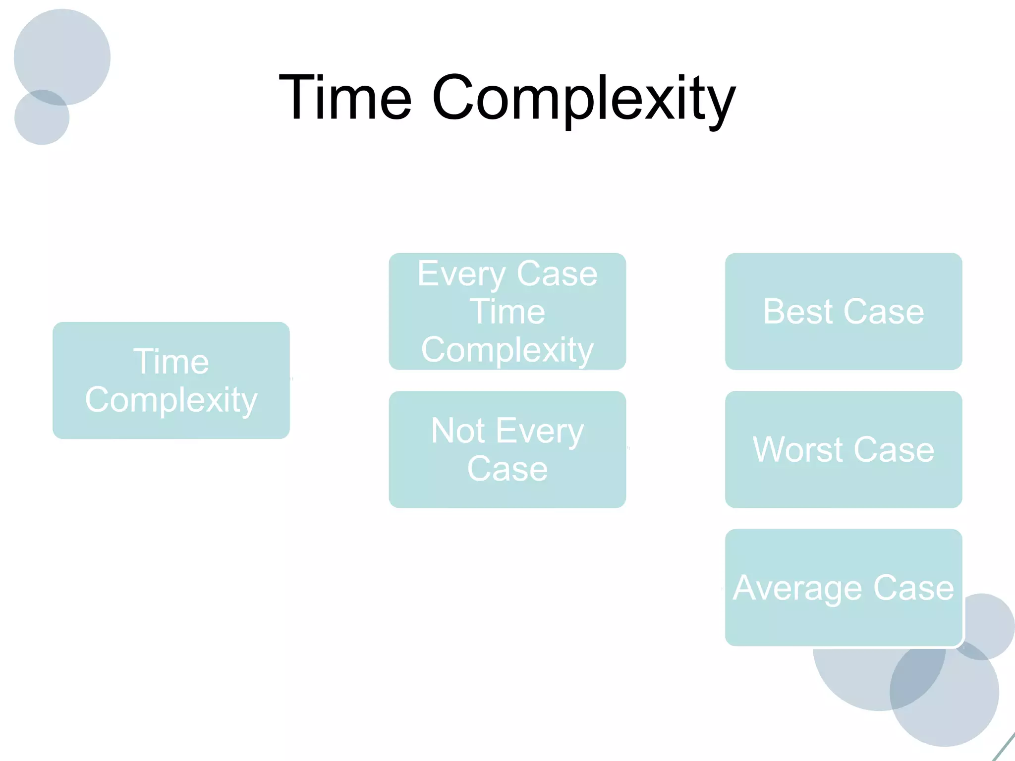

![Every case time
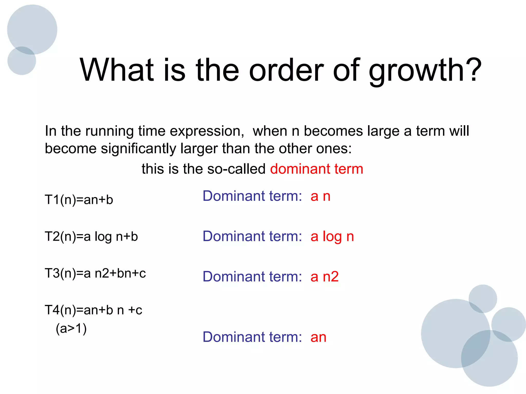
Complexity(examples)
• Sum of elements of array
Algorithm sum_array(A,n)
sum=0
for i=1 to n
sum+=A[i]
return sum](https://image.slidesharecdn.com/02-orderofgrowth-150601060814-lva1-app6891/75/02-order-of-growth-21-2048.jpg)

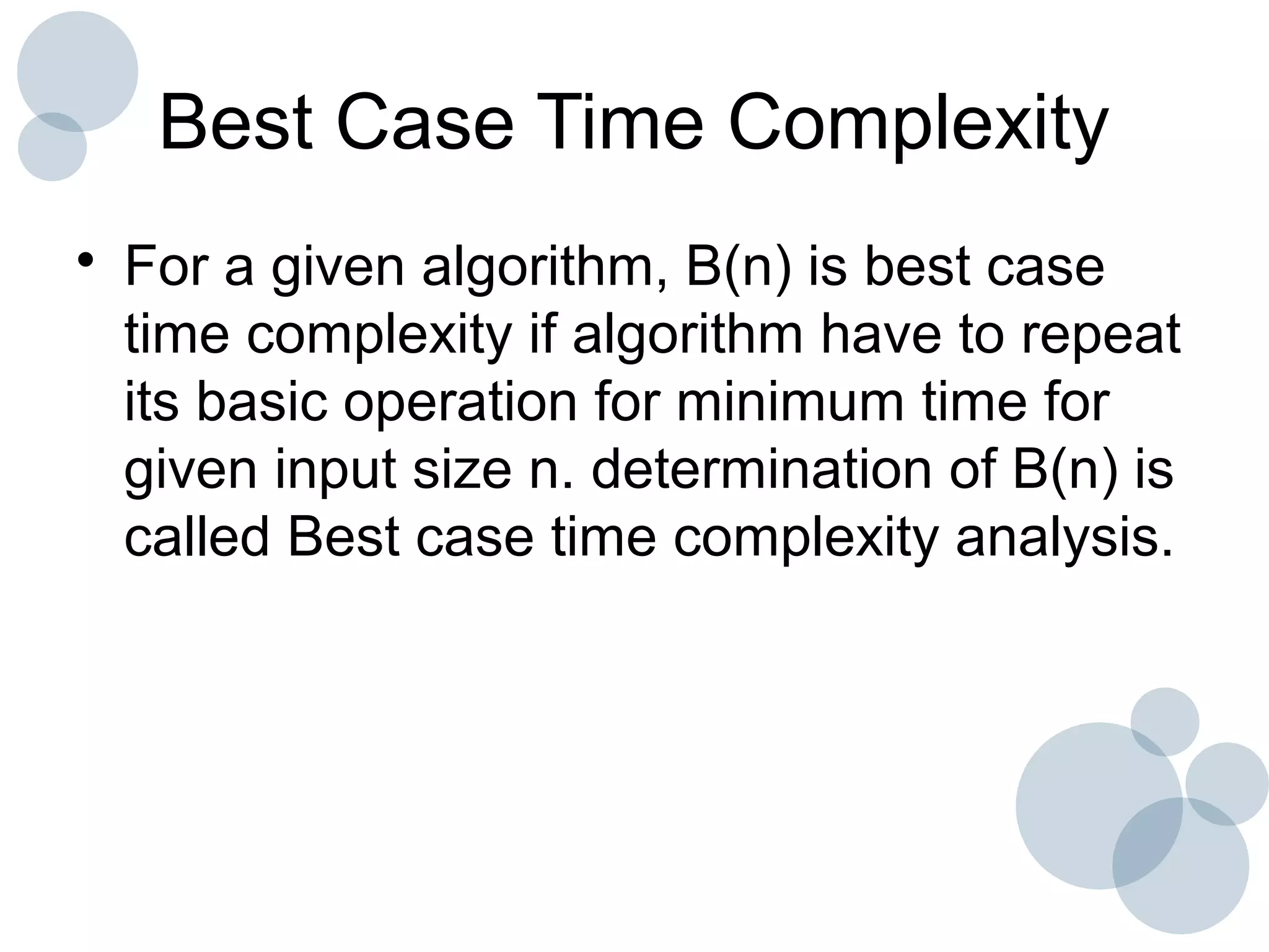
![Every case time
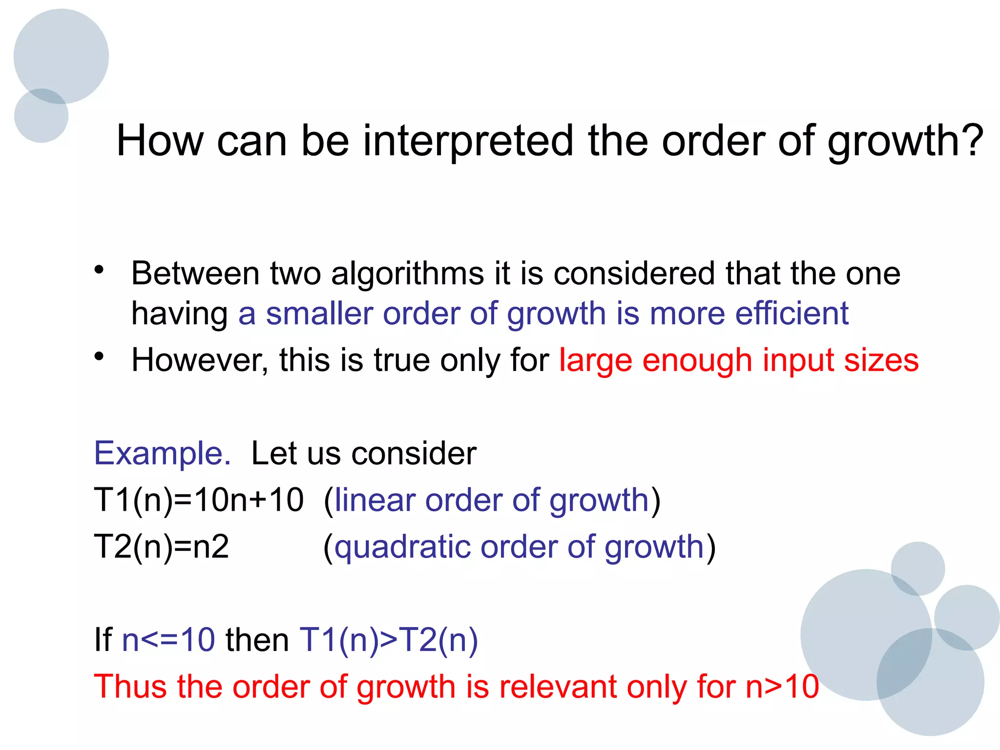
Complexity(examples)
• Exchange Sort
Algorithm exchange_sort(A,n)
for i=1 to n-1
for j= i+1 to n
if A[i]>A[j]
exchange A[i] &A[j]](https://image.slidesharecdn.com/02-orderofgrowth-150601060814-lva1-app6891/75/02-order-of-growth-23-2048.jpg)

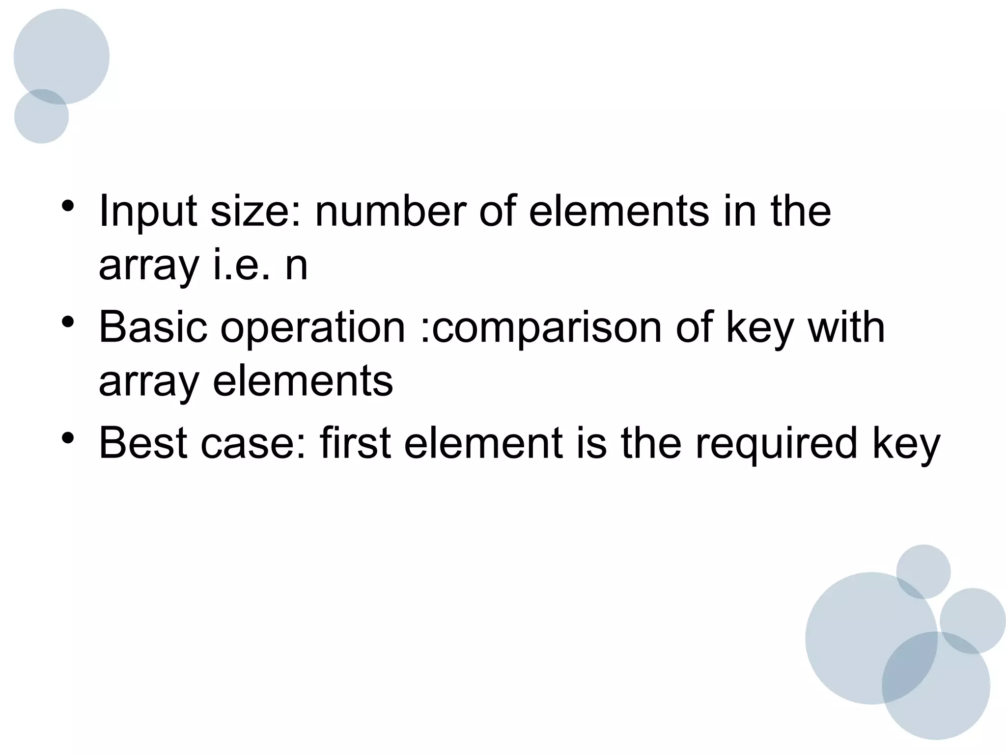
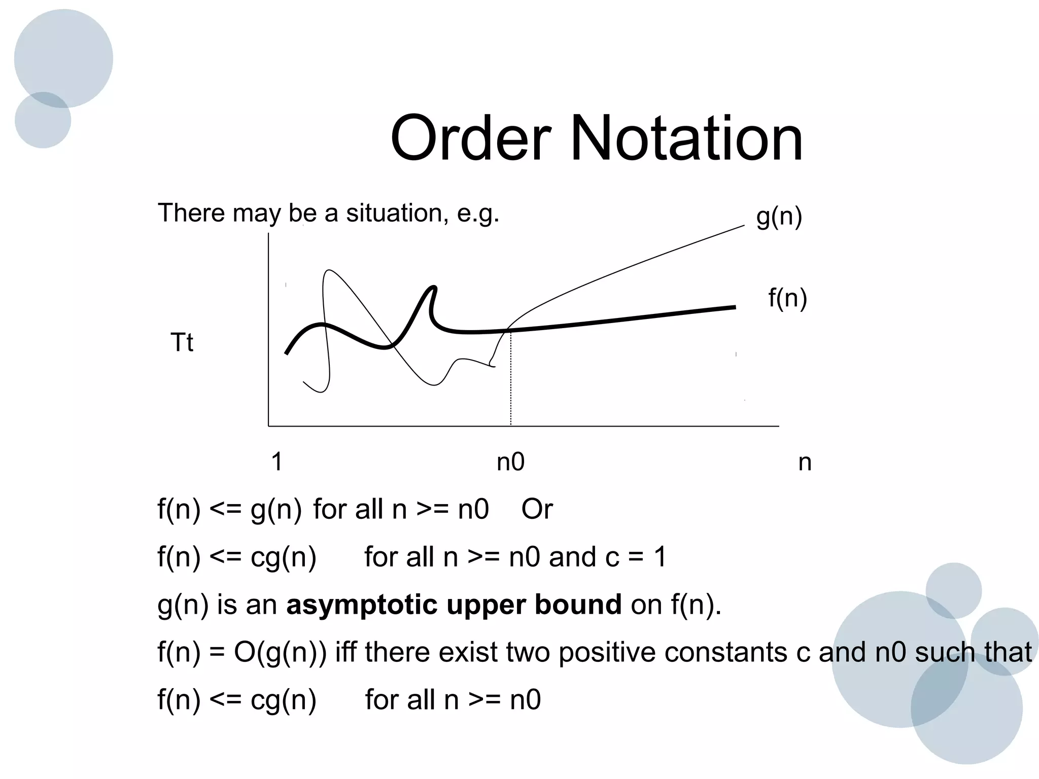
![Best Case Time Complexity
(Example)
Algorithm sequential_search(A,n,key)
i=0
while i<n && A[i]!= key
i=i+1
If i<n
return i
Else return-1](https://image.slidesharecdn.com/02-orderofgrowth-150601060814-lva1-app6891/75/02-order-of-growth-26-2048.jpg)

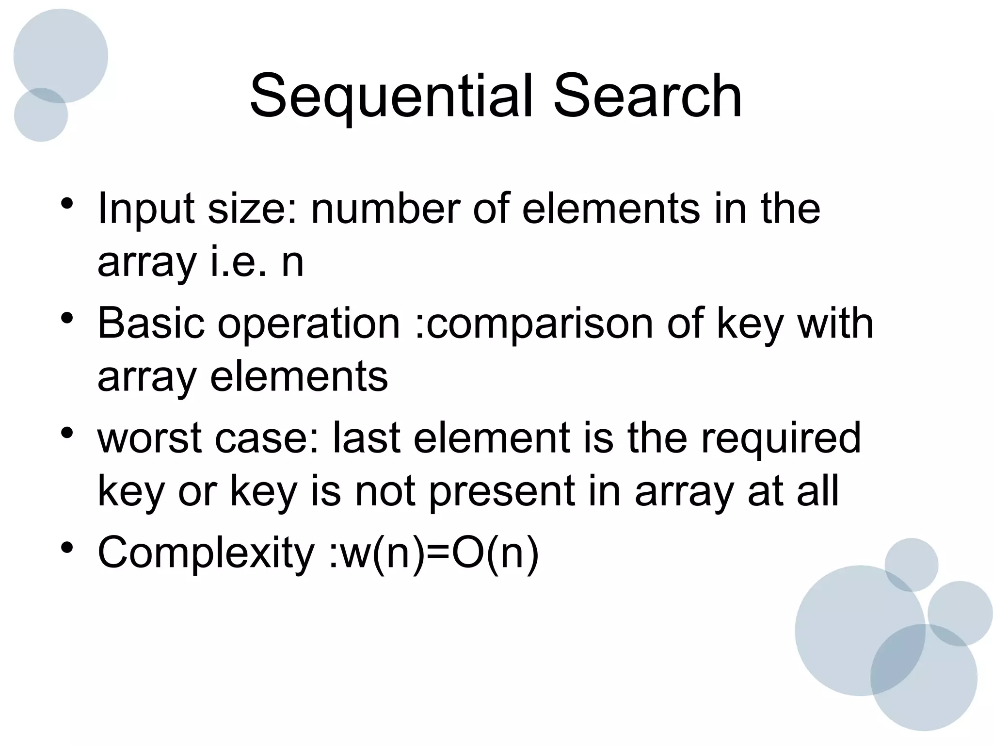


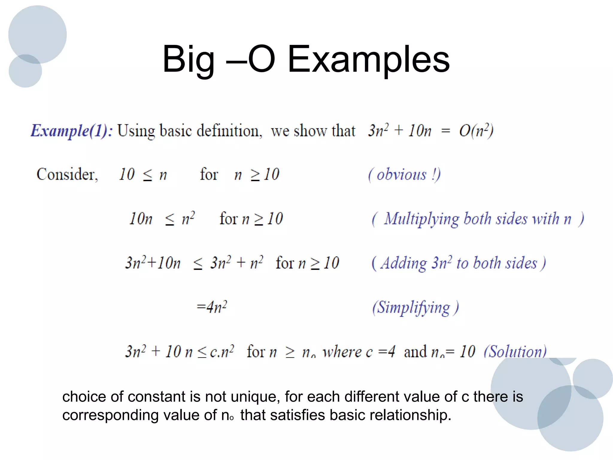
![• Average case: probability of successful
search is p(0<=p<=1)
• Probability of each element is p/n
multiplied with number of comparisons ie
• p/n*i
• A(n)=[1.p/n+2.p/n+…..n.p/n]+n.(1-p)
p/n(1+2+3+…+n)+n.(1-p)
P(n+1)/2 +n(1-p)](https://image.slidesharecdn.com/02-orderofgrowth-150601060814-lva1-app6891/75/02-order-of-growth-32-2048.jpg)


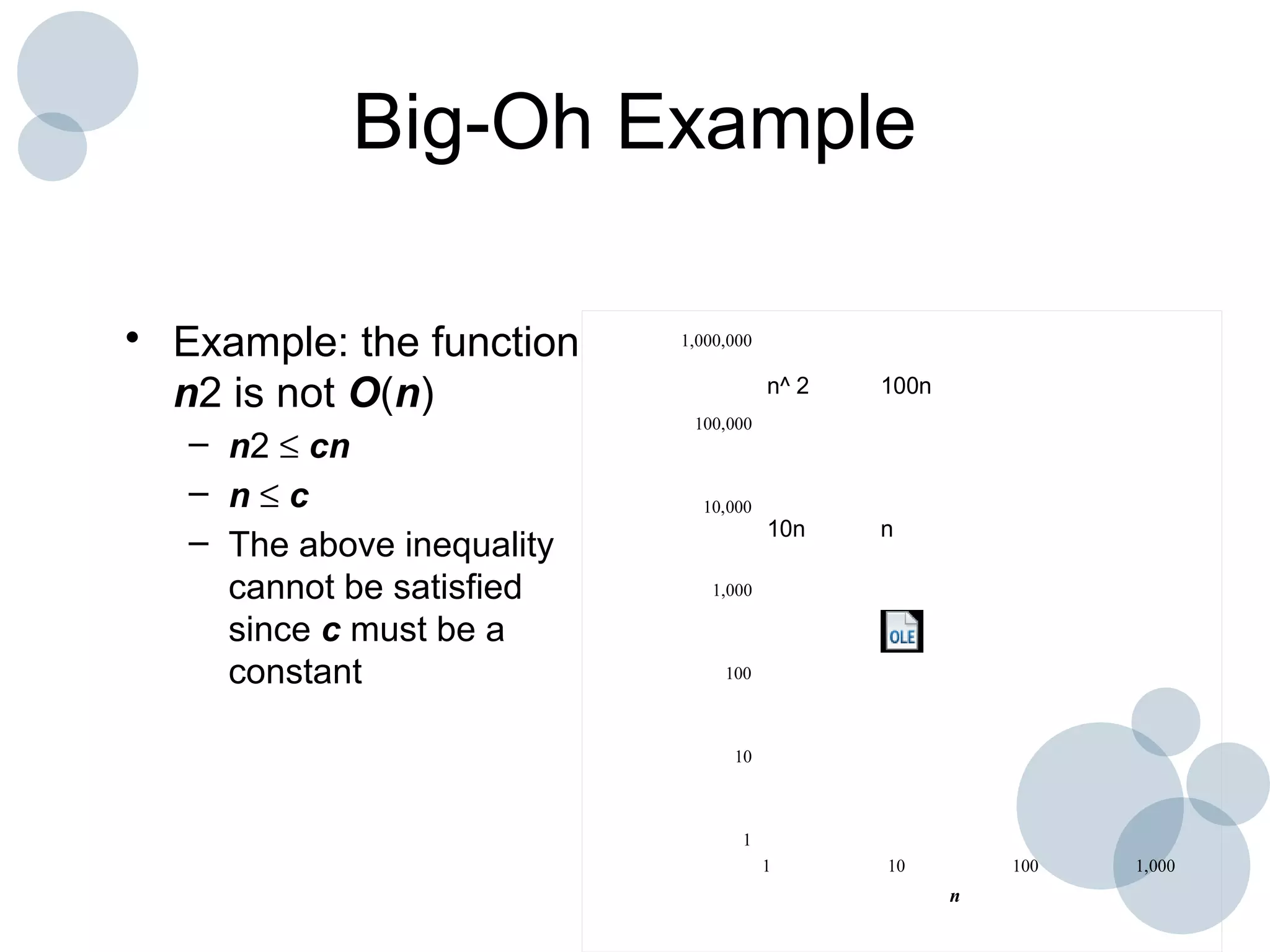


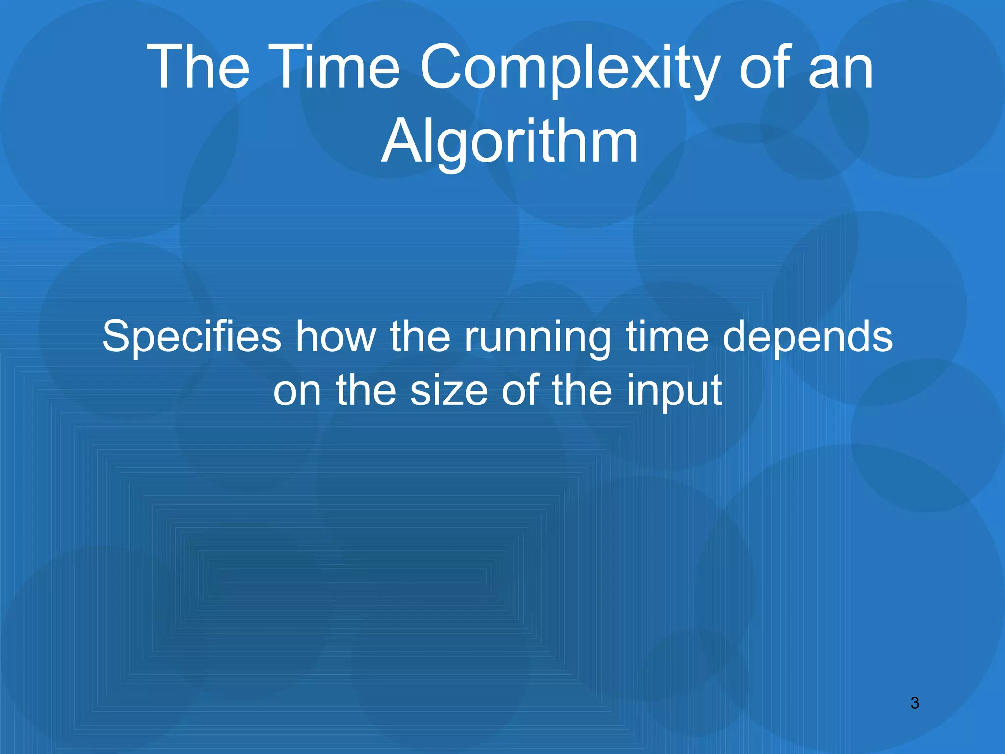
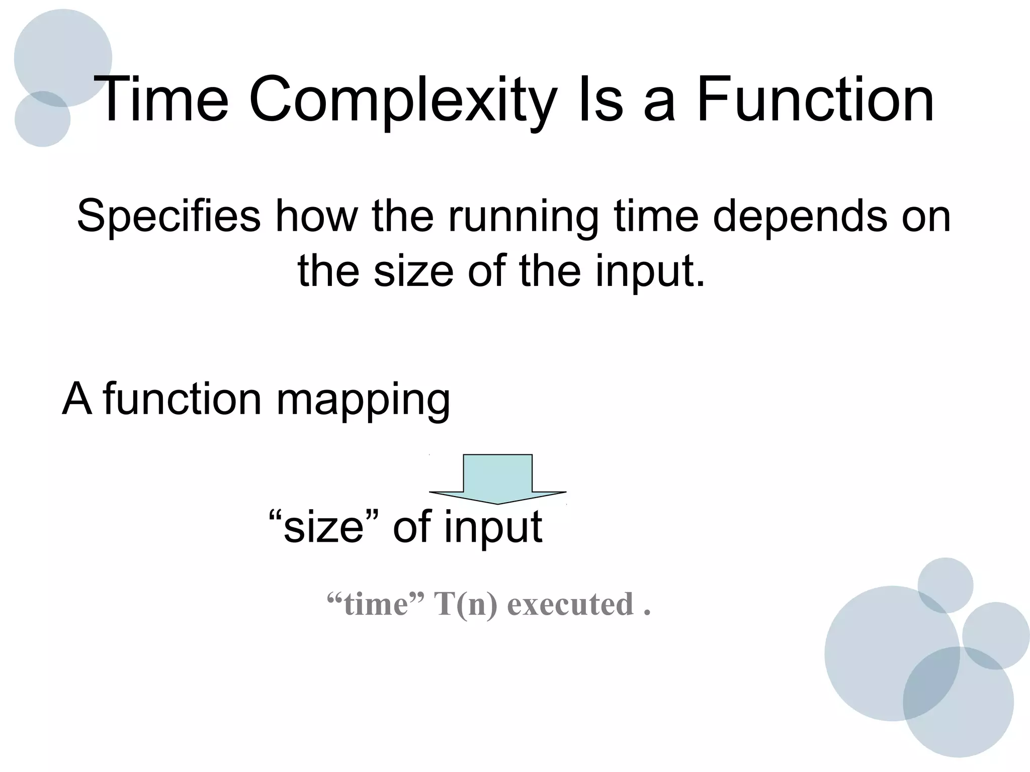
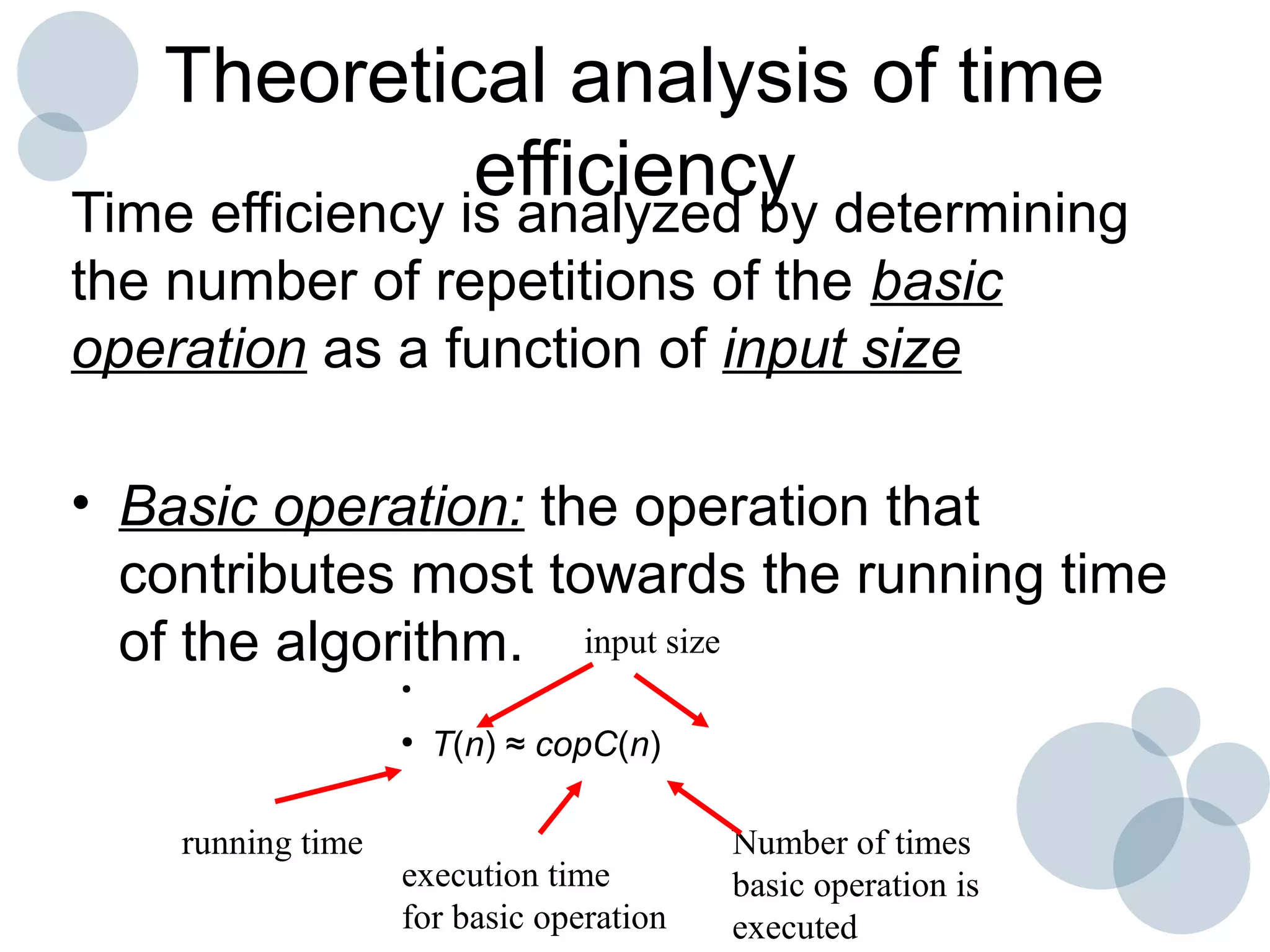
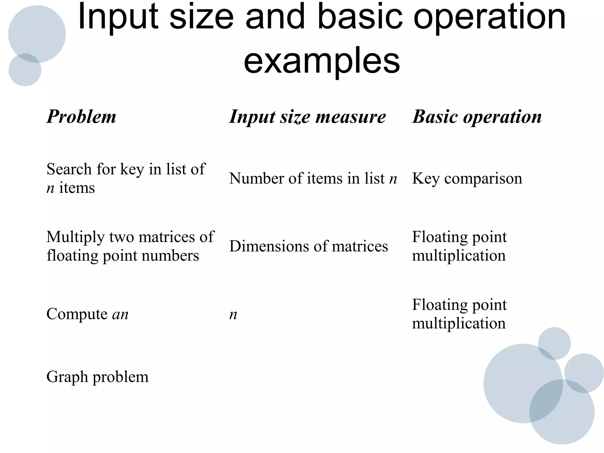
Time complexity analysis specifies how the running time of an algorithm depends on the size of its input. It is determined by identifying the basic operation of the algorithm and counting how many times it is executed as the input size increases. The time complexity of an algorithm can be expressed as a function T(n) relating the input size n to the running time. Common time complexities include constant O(1), linear O(n), logarithmic O(log n), and quadratic O(n^2). The order of growth indicates how fast the running time grows as n increases and is used to compare the efficiency of algorithms.