Download as PDF, PPTX

![● Example: evaluate f= x2
+ y2
. First define the graph.
import tensorflow as tf
x = tf.Variable( 3)
y = tf.Variable( 4)
f = x*x + y*y
● It’s separated from its execution:
>>> sess = tf.Session()
>>> sess.run(x.initializer)
>>> sess.run(y.initializer)
>>> result = sess.run() # Result equals 25
● Or more compactly:
init = tf.global_variables_initializer()
with tf.Session() as sess:
init.run()
result = f.eval
12
Deep Learning with TensorFlow
● Example:Graph for Logistic Regression on the MNIST database.
# Data input
x = tf.placeholder(tf.float32, [ None, 784])
y = tf.placeholder(tf.float32, [ None, 10])
# Set model weights
W = tf.Variable(tf.zeros([ 784, 10]))
b = tf.Variable(tf.zeros([ 10]))
# Construct model
pred = tf.nn.softmax(tf.matmul(x, W) + b) # Softmax
# Minimize error using cross entropy
cost = tf.reduce_mean( -tf.reduce_sum(y *tf.log(pred), axis=1))
# Gradient Descent
optimizer = tf.train.GradientDescentOptimizer(learning_rate)
.minimize(cost)
● Running and optimising:
with tf.Session() as sess:
sess.run(init)
for i in range(total_batch):
batch_xs, batch_ys = mnist.train.next_batch(batch_size)
_, c = sess.run([optimizer, cost], feed_dict ={x: batch_xs,
y: batch_ys})
# Compute average loss
avg_cost += c / total_batch
TensorFlow is a open source software library for numerical computation.](https://image.slidesharecdn.com/presentacionpycones2017-170925101327/85/Python-Tensorflow-how-to-earn-money-in-the-Stock-Exchange-with-Deep-Learning-PyconEs2017-talk-12-320.jpg)
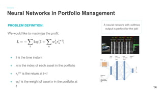
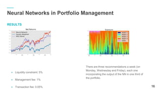

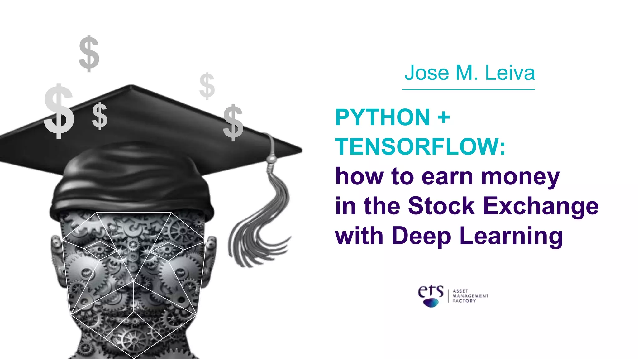
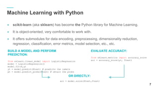
The document discusses using Python and TensorFlow for deep learning applications in stock exchange trading and asset management. It covers foundational concepts in machine learning, including neural networks, training models, and performance evaluation, along with practical examples. Additionally, it explores the use of neural networks in portfolio management to maximize profits while incorporating various constraints.


![[신경망기초] 합성곱신경망](https://cdn.slidesharecdn.com/ss_thumbnails/2-180604135842-thumbnail.jpg?width=640&height=640&fit=bounds)

![[신경망기초]오류역전파알고리즘구현](https://cdn.slidesharecdn.com/ss_thumbnails/nn-190319093725-thumbnail.jpg?width=640&height=640&fit=bounds)