Download as PDF, PPTX


![8
8
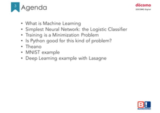
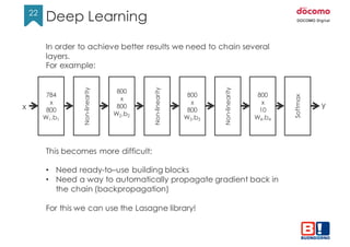
To create a classifier we want the output y to look like a set of
probabilities. For example:
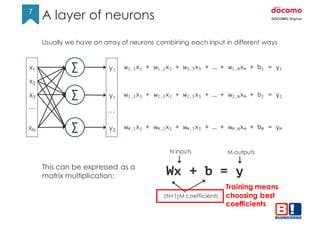
x1
x2
x3
xN
…
Σ
Σ
Σ
Y1 = 2
Y1 = 0.6
Y3 = 0.1
…
Is it a cat?
Is it a dog?
Is it a fish?
We have a set of scores y called ”logits” but in this version they
cannot be used as probabilities because:
• The are not values in the range [0,1]
• They do not add up to 1
Example](https://image.slidesharecdn.com/neuralnetworkswithpython-160419073810/85/Neural-networks-with-python-8-320.jpg)
![9
9
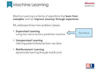
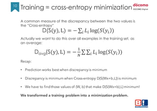
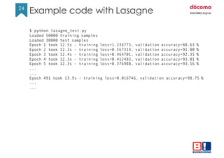
To convert logits into probabilities we can use the Softmax function:
S(𝑦𝑖) =
&'(
∑ &'
This guarantees all values are between [0,1] and they add up to 1.
At this point we can compare the result of a prediction with the expected
value coming from the label.
This is a cat so the ideal result should be [1,0,0]
x1
x2
x3
xN
…
Σ
Σ
Σ
Y1
Y2
Y3
softmax
0.72
0.18
0.10
S(y)
1
0
0
Label
(one-hot)
≠
Ideally S(y) == Label
Training means making S(y) as close to Label as possible.
Softmax and cross-entropy](https://image.slidesharecdn.com/neuralnetworkswithpython-160419073810/85/Neural-networks-with-python-9-320.jpg)

![14
14
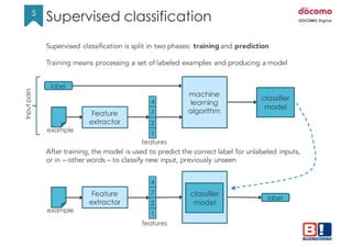
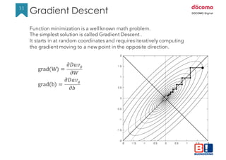
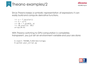
from theano import function
import theano.tensor as T
a = T.dscalar()
b = T.dscalar()
c = a + b
f = theano.function([a,b], c)
assert 4.0 == f(1.5, 2.5)
A simple program to build a symbolic expression and run a computation
Note: Theano builds a symbolic representation of the math behind the function
so the expression can be manipulated or rearranged dynamically before the
actual computation happens.
Same happens for matrixes
x = T.dmatrix('x') # you can give a symbolic name to the variable
y = T.dmatrix('y')
z = x + y
f = function([x, y], z)
assert numpy.all(f([[1, 2],[3, 4]], [[10,20],[30,40]]) ==
numpy.array([[11.,22.],[33.,44.]]))
Theano examples/1](https://image.slidesharecdn.com/neuralnetworkswithpython-160419073810/85/Neural-networks-with-python-14-320.jpg)
![18
18
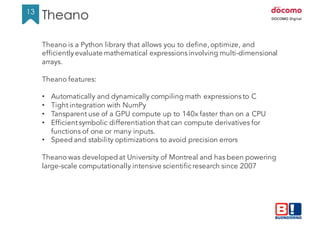
import theano
import theano.tensor as T
class NN1Layer(object):
def __init__(self, n_in, n_out, learning_rate=1.0):
# create two symbolic variables for our model
x = T.matrix('x') # matrix of [784, nsamples] input pixels
y = T.ivector('y') # 1D vector of [nsamples] output labels
# create the coefficient matrixes, pre-filled with zeros
self.W = theano.shared(value=numpy.zeros((n_in, n_out)))
self.b = theano.shared(value=numpy.zeros((n_out,)))
# expression of label probabilities
p_y_given_x = T.nnet.softmax(T.dot(x, self.W) + self.b)
# expression for the cost function
cost = -T.mean(T.log(p_y_given_x)[T.arange(y.shape[0]), y])
Example MNIST – The code/1](https://image.slidesharecdn.com/neuralnetworkswithpython-160419073810/85/Neural-networks-with-python-18-320.jpg)
![19
19
# gradients of the cost over the coefficients
grad_W = T.grad(cost=cost, wrt=self.W)
grad_b = T.grad(cost=cost, wrt=self.b)
updates = [(self.W, self.W - learning_rate * grad_W),
(self.b, self.b - learning_rate * grad_b)]
# the function for training
self.train_model = theano.function([x, y], cost,
updates=updates, allow_input_downcast=True)
# expression for prediction
y_pred = T.argmax(p_y_given_x, axis=1)
# the function for prediction
self.predict_model = theano.function([x], y_pred)
Example MNIST – The code/2](https://image.slidesharecdn.com/neuralnetworkswithpython-160419073810/85/Neural-networks-with-python-19-320.jpg)
![20
20
def train(self, data_x, data_y, val_x, val_y, n_epochs=1000):
for epoch in range(n_epochs):
avg_cost = self.train_model(data_x, data_y)
precision = 100*self.validate(val_x, val_y)
print("Epoch {}, cost={:.6f}, precision={:.2f}%”.format(
epoch, avg_cost, precision))
def predict(self, data_x):
return self.predict_model(data_x)
def validate(self, data_x, data_y):
# execute a prediction and check how many results are OK
pred_y = self.predict(data_x)
nr_good = 0
for i in range(len(data_y)):
if pred_y[i] == data_y[i]:
nr_good += 1
return 1.0*nr_good/len(data_y)
Example MNIST – The code/3](https://image.slidesharecdn.com/neuralnetworkswithpython-160419073810/85/Neural-networks-with-python-20-320.jpg)
![23
23
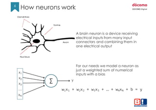
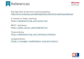
Example code with Lasagne
import lasagne
import lasagne.layers as LL
Import lasagne.nonlinearities as LNL
class MultiLayerPerceptron(object):
def __init__(self):
x = T.matrix('x')
y = T.ivector(’y')
network = self.build_mlp(x)
pred1 = network.get_output()
cost = lasagne.objectives.categorical_crossentropy(pred1, y).mean()
params = LL.get_all_params(network)
updates = lasagne.updates.nesterov_momentum(
cost, params, learning_rate=0.01, momentum=0.9)
self.train_model = theano.function([x, y], cost, updates=updates)
pred2 = network.get_output(deterministic=True)
self.prediction_model = theano.function([x, y], pred2)
def build_mlp(self, x):
l1 = LL.InputLayer(shape=(None, 784), input_var=x)
l2 = LL.DropoutLayer(l1, p=0.2)
l3 = LL.DenseLayer(l2, num_units=800, nonlinearity=LNL.rectify)
l4 = LL.DropoutLayer(l3, p=0.5)
l5 = LL.DenseLayer(l4, num_units=800, nonlinearity=LNL.rectify)
l6 = LL.DropoutLayer(l5, p=0.5)
return LL.DenseLayer(l6, num_units=10, nonlinearity=LNL.softmax)](https://image.slidesharecdn.com/neuralnetworkswithpython-160419073810/85/Neural-networks-with-python-23-320.jpg)


This document discusses neural networks in Python using Theano and Lasagne libraries. It begins with an introduction to machine learning concepts like supervised learning and neural network training as minimizing a cost function. It then demonstrates how to build and train a simple neural network classifier for MNIST digits using Theano. Finally, it shows how to build a deeper multi-layer network for MNIST using Lasagne, obtaining better results through multiple layers and dropout regularization.