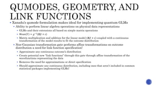
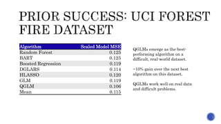
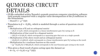
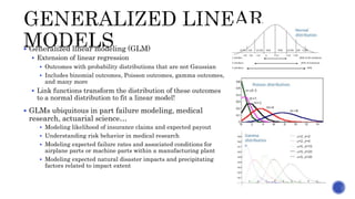
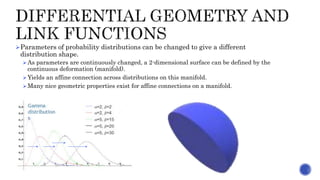
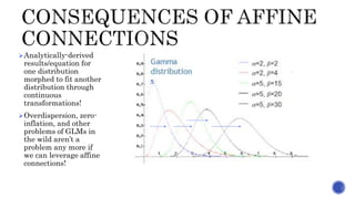
Colleen M. Farrelly and Uchenna Chukwu
 Generalized linear modeling (GLM)
 Extension of linear regression
 Outcomes with probability distributions that are not Gaussian
 Includes binomial outcomes, Poisson outcomes, gamma outcomes,
and many more
 Link functions transform the distribution of these outcomes
to a normal distribution to fit a linear model!
 GLMs ubiquitous in part failure modeling, medical
research, actuarial science…
 Modeling likelihood of insurance claims and expected payout
 Understanding risk behavior in medical research
 Modeling expected failure rates and associated conditions for
airplane parts or machine parts within a manufacturing plant
 Modeling expected natural disaster impacts and precipitating
factors related to impact extent
 Many supervised learning algorithm extensions
 Link function
 Either directly specified and modeled
 Or estimated during the algorithm
 Examples
 Boosted regression, Morse-Smale regression, dgLARS, Bayesian
model averaging…
 Dealing with the link function in machine learning
 Various optimization algorithms to find minimum sum of square
error
 Series of general mappings leading to a potentially novel link
function through deep learning
 Models struggle when distribution has a lot of 0’s or
outliers.
 Alternative approach:
1. Exploit the geometric relationships between distributions
2. Superpose these distributions
3. Collapse to the “ideal” link
Parameters of probability distributions can be changed to give a different
distribution shape.
As parameters are continuously changed, a 2-dimensional surface can be defined by the
continuous deformation (manifold).
Yields an affine connection across distributions on this manifold.
Many nice geometric properties exist for affine connections on a manifold.
Analytically-derived
results/equation for
one distribution
morphed to fit another
distribution through
continuous
transformations!
Overdispersion, zero-
inflation, and other
problems of GLMs in
the wild aren’t a
problem any more if
we can leverage affine
connections!
 Xanadu’s qumode formulation makes ideal for implementing quantum GLMs
 Ability to perform linear algebra operations on physical data representations
 GLMs and their extensions all based on simple matrix operations
 𝑀𝑒𝑎𝑛 𝑌 = 𝑔−1
𝑿𝛽 + 𝜀
 Matrix multiplication and addition for the linear model 𝑿𝛽 + 𝜀 coupled with a continuous
transformation of the model results to fit the outcome distribution
 Non-Gaussian transformation gate performs affine transformations on outcome
distribution a need for link function specification!
 Approximate any continuous outcome’s distribution
 Create potential new “link functions” through this gate through affine transformation of the
wavefunctions representing the data
 Removes the need for approximations or direct specification
 Should approximate any continuous distribution, including ones that aren’t included in common
statistical packages implementing GLMs!
Algorithm Scaled Model MSE
Random Forest 0.125
BART 0.125
Boosted Regression 0.119
DGLARS 0.114
HLASSO 0.120
GLM 0.119
QGLM 0.106
Mean 0.115
QGLMs emerge as the best-
performing algorithm on a
difficult, real-world dataset.
~10% gain over the next best
algorithm on this dataset.
QGLMs work well on real data
and difficult problems.
 GLMs embedded within Xanadu’s qumode quantum computer simulation software
(and qumode computer) with a singular value decomposition of the 𝛽 coefficient in
the formulation:
 𝑀𝑒𝑎𝑛 𝑌 = 𝑔−1 𝑋𝛽
 Translates to 𝛽 = 𝑂1Σ𝑂2, which is modeled through a series of quantum circuit
gates:
 Multiplication of X and an orthogonal matrix:
 | 𝑂1 𝑋 ≅ 𝑈1| 𝑋 , which corresponds to a linear interferometer gate (𝑈1) acting on X
 Multiplication of that result by a diagonal matrix:
 |Σ𝑂1 𝑋 ∝ 𝑆 𝑟 | 𝑂1 𝑋 , which corresponds to a squeezing gate that acts on a single qumode
 Multiplication of the above result and an orthogonal matrix:
 | 𝑂2Σ𝑂1 𝑋 ≅ 𝑈2|Σ 𝑂1 𝑋 , which corresponds to a linear interferometer gate (𝑈2) acting on the result
 Multiplication by a nonlinear function on this result:
 |𝑔−1
( 𝑂2Σ𝑂1 𝑋) ≅ Φ|𝑂2Σ𝑂1 𝑋 , which corresponds to the non-Gaussian gate acting on the result
 This gives a final result of gates acting upon the dataset as:
 Φ ∗ 𝒰2 ∗ 𝒮 ∗ 𝒰1| 𝑋 ∝ | 𝑔−1
𝑋𝛽
 Data used will include a small subset of the processed UCI dataset (reduced
dimension).
 Code implemented through Strawberry Fields package in Python:
 Use pandas data frame to read csv files of training and test data for UCI Forest
Fire.
 Shuffled training and test data set and took only the first 30 and 10 rows,
respectively. Both data sets have 4 features and 1 output.
 Learning rate = 0.1
 Mean-squared error loss function
 Stochastic Gradient Descent
 Batch size = 10
 Iterations = 50
 For training size = 30 and test size = 10, mean-squared error for test equals 0.152
 Jorgensen, B. (1997). The theory of dispersion models. CRC Press.
 Jørgensen, B., Goegebeur, Y., & Martínez, J. R. (2010). Dispersion models for extremes. Extremes, 13(4), 399-437.
 Killoran, N., Bromley, T. R., Arrazola, J. M., Schuld, M., Quesada, N., & Lloyd, S. (2018). Continuous-variable quantum
neural networks. arXiv preprint arXiv:1806.06871.
 Killoran, N., Izaac, J., Quesada, N., Bergholm, V., Amy, M., & Weedbrook, C. (2018). Strawberry Fields: A Software
Platform for Photonic Quantum Computing. arXiv preprint arXiv:1804.03159.
 Luitel, B. N. (2016). Prediction of North Atlantic tropical cyclone activity and rainfall (Doctoral dissertation, The University
of Iowa).
 Marriott, P. (1990). Applications of differential geometry to statistics (Doctoral dissertation, University of Warwick).
 Mills, K. L., Teesson, M., Ross, J., & Peters, L. (2006). Trauma, PTSD, and substance use disorders: findings from the
Australian National Survey of Mental Health and Well-Being. American Journal of Psychiatry, 163(4), 652-658.
 Nielsen, F., & Garcia, V. (2009). Statistical exponential families: A digest with flash cards. arXiv preprint arXiv:0911.4863.
 Osborne, M. R., Presnell, B., & Turlach, B. A. (2000). A new approach to variable selection in least squares problems. IMA
journal of numerical analysis, 20(3), 389-403.
 Pistone, G., & Rogantin, M. P. (1999). The exponential statistical manifold: mean parameters, orthogonality and space
transformations. Bernoulli, 5(4), 721-760.
 Sawalha, Z., & Sayed, T. (2006). Traffic accident modeling: some statistical issues. Canadian Journal of Civil Engineering,
33(9), 1115-1124.
 Tweedie, M. C. K. (1984). An index which distinguishes between some important exponential families. In Statistics:
Applications and new directions: Proc. Indian statistical institute golden Jubilee International conference (Vol. 579, p. 6o4).

PyData Miami 2019, Quantum Generalized Linear Models

  • 1.
    Colleen M. Farrellyand Uchenna Chukwu
  • 2.
     Generalized linearmodeling (GLM)  Extension of linear regression  Outcomes with probability distributions that are not Gaussian  Includes binomial outcomes, Poisson outcomes, gamma outcomes, and many more  Link functions transform the distribution of these outcomes to a normal distribution to fit a linear model!  GLMs ubiquitous in part failure modeling, medical research, actuarial science…  Modeling likelihood of insurance claims and expected payout  Understanding risk behavior in medical research  Modeling expected failure rates and associated conditions for airplane parts or machine parts within a manufacturing plant  Modeling expected natural disaster impacts and precipitating factors related to impact extent
  • 3.
     Many supervisedlearning algorithm extensions  Link function  Either directly specified and modeled  Or estimated during the algorithm  Examples  Boosted regression, Morse-Smale regression, dgLARS, Bayesian model averaging…  Dealing with the link function in machine learning  Various optimization algorithms to find minimum sum of square error  Series of general mappings leading to a potentially novel link function through deep learning  Models struggle when distribution has a lot of 0’s or outliers.  Alternative approach: 1. Exploit the geometric relationships between distributions 2. Superpose these distributions 3. Collapse to the “ideal” link
  • 4.
    Parameters of probabilitydistributions can be changed to give a different distribution shape. As parameters are continuously changed, a 2-dimensional surface can be defined by the continuous deformation (manifold). Yields an affine connection across distributions on this manifold. Many nice geometric properties exist for affine connections on a manifold.
  • 5.
    Analytically-derived results/equation for one distribution morphedto fit another distribution through continuous transformations! Overdispersion, zero- inflation, and other problems of GLMs in the wild aren’t a problem any more if we can leverage affine connections!
  • 6.
     Xanadu’s qumodeformulation makes ideal for implementing quantum GLMs  Ability to perform linear algebra operations on physical data representations  GLMs and their extensions all based on simple matrix operations  𝑀𝑒𝑎𝑛 𝑌 = 𝑔−1 𝑿𝛽 + 𝜀  Matrix multiplication and addition for the linear model 𝑿𝛽 + 𝜀 coupled with a continuous transformation of the model results to fit the outcome distribution  Non-Gaussian transformation gate performs affine transformations on outcome distribution a need for link function specification!  Approximate any continuous outcome’s distribution  Create potential new “link functions” through this gate through affine transformation of the wavefunctions representing the data  Removes the need for approximations or direct specification  Should approximate any continuous distribution, including ones that aren’t included in common statistical packages implementing GLMs!
  • 7.
    Algorithm Scaled ModelMSE Random Forest 0.125 BART 0.125 Boosted Regression 0.119 DGLARS 0.114 HLASSO 0.120 GLM 0.119 QGLM 0.106 Mean 0.115 QGLMs emerge as the best- performing algorithm on a difficult, real-world dataset. ~10% gain over the next best algorithm on this dataset. QGLMs work well on real data and difficult problems.
  • 8.
     GLMs embeddedwithin Xanadu’s qumode quantum computer simulation software (and qumode computer) with a singular value decomposition of the 𝛽 coefficient in the formulation:  𝑀𝑒𝑎𝑛 𝑌 = 𝑔−1 𝑋𝛽  Translates to 𝛽 = 𝑂1Σ𝑂2, which is modeled through a series of quantum circuit gates:  Multiplication of X and an orthogonal matrix:  | 𝑂1 𝑋 ≅ 𝑈1| 𝑋 , which corresponds to a linear interferometer gate (𝑈1) acting on X  Multiplication of that result by a diagonal matrix:  |Σ𝑂1 𝑋 ∝ 𝑆 𝑟 | 𝑂1 𝑋 , which corresponds to a squeezing gate that acts on a single qumode  Multiplication of the above result and an orthogonal matrix:  | 𝑂2Σ𝑂1 𝑋 ≅ 𝑈2|Σ 𝑂1 𝑋 , which corresponds to a linear interferometer gate (𝑈2) acting on the result  Multiplication by a nonlinear function on this result:  |𝑔−1 ( 𝑂2Σ𝑂1 𝑋) ≅ Φ|𝑂2Σ𝑂1 𝑋 , which corresponds to the non-Gaussian gate acting on the result  This gives a final result of gates acting upon the dataset as:  Φ ∗ 𝒰2 ∗ 𝒮 ∗ 𝒰1| 𝑋 ∝ | 𝑔−1 𝑋𝛽
  • 9.
     Data usedwill include a small subset of the processed UCI dataset (reduced dimension).  Code implemented through Strawberry Fields package in Python:
  • 10.
     Use pandasdata frame to read csv files of training and test data for UCI Forest Fire.  Shuffled training and test data set and took only the first 30 and 10 rows, respectively. Both data sets have 4 features and 1 output.
  • 11.
     Learning rate= 0.1  Mean-squared error loss function  Stochastic Gradient Descent  Batch size = 10  Iterations = 50
  • 13.
     For trainingsize = 30 and test size = 10, mean-squared error for test equals 0.152
  • 14.
     Jorgensen, B.(1997). The theory of dispersion models. CRC Press.  Jørgensen, B., Goegebeur, Y., & Martínez, J. R. (2010). Dispersion models for extremes. Extremes, 13(4), 399-437.  Killoran, N., Bromley, T. R., Arrazola, J. M., Schuld, M., Quesada, N., & Lloyd, S. (2018). Continuous-variable quantum neural networks. arXiv preprint arXiv:1806.06871.  Killoran, N., Izaac, J., Quesada, N., Bergholm, V., Amy, M., & Weedbrook, C. (2018). Strawberry Fields: A Software Platform for Photonic Quantum Computing. arXiv preprint arXiv:1804.03159.  Luitel, B. N. (2016). Prediction of North Atlantic tropical cyclone activity and rainfall (Doctoral dissertation, The University of Iowa).  Marriott, P. (1990). Applications of differential geometry to statistics (Doctoral dissertation, University of Warwick).  Mills, K. L., Teesson, M., Ross, J., & Peters, L. (2006). Trauma, PTSD, and substance use disorders: findings from the Australian National Survey of Mental Health and Well-Being. American Journal of Psychiatry, 163(4), 652-658.  Nielsen, F., & Garcia, V. (2009). Statistical exponential families: A digest with flash cards. arXiv preprint arXiv:0911.4863.  Osborne, M. R., Presnell, B., & Turlach, B. A. (2000). A new approach to variable selection in least squares problems. IMA journal of numerical analysis, 20(3), 389-403.  Pistone, G., & Rogantin, M. P. (1999). The exponential statistical manifold: mean parameters, orthogonality and space transformations. Bernoulli, 5(4), 721-760.  Sawalha, Z., & Sayed, T. (2006). Traffic accident modeling: some statistical issues. Canadian Journal of Civil Engineering, 33(9), 1115-1124.  Tweedie, M. C. K. (1984). An index which distinguishes between some important exponential families. In Statistics: Applications and new directions: Proc. Indian statistical institute golden Jubilee International conference (Vol. 579, p. 6o4).

Editor's Notes

  • #5 Marriott, P. (1990). Applications of differential geometry to statistics (Doctoral dissertation, University of Warwick). Nielsen, F., & Garcia, V. (2009). Statistical exponential families: A digest with flash cards. arXiv preprint arXiv:0911.4863. Amari, S. I. (1997). Information geometry. Contemporary Mathematics, 203, 81-96. Pistone, G., & Rogantin, M. P. (1999). The exponential statistical manifold: mean parameters, orthogonality and space transformations. Bernoulli, 5(4), 721-760.
  • #6 Jørgensen, B., & Martínez, J. R. (2013, March). Multivariate exponential dispersion models. In Multivariate Statistics: Theory and Applications. Proceedings of the IX Tartu Conference on Multivariate Statistics & XX International Workshop on Matrices and Statistics (pp. 73-98). Jorgensen, B. (1997). The theory of dispersion models. CRC Press. Sawalha, Z., & Sayed, T. (2006). Traffic accident modeling: some statistical issues. Canadian Journal of Civil Engineering, 33(9), 1115-1124. Jørgensen, B., Goegebeur, Y., & Martínez, J. R. (2010). Dispersion models for extremes. Extremes, 13(4), 399-437. Marriott, P. (1990). Applications of differential geometry to statistics (Doctoral dissertation, University of Warwick).