This document provides an introduction to pumping stations, including:
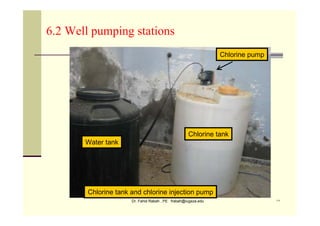
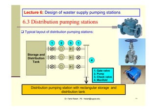
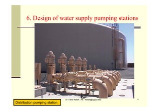
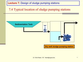
- The main purposes of pumping stations are to transfer fluids from low to high points, with main types being wastewater, water, sludge, and storm water pumping stations.
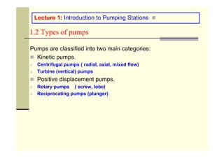
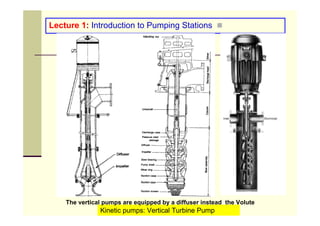
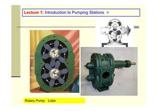
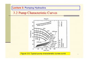
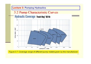
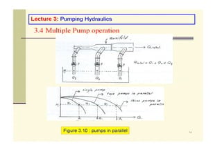
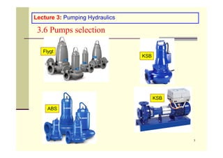
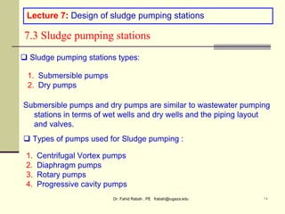
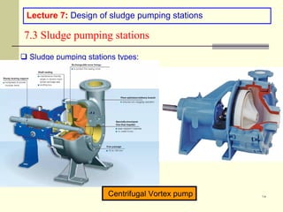
- Pumps are classified as kinetic (centrifugal, turbine) or positive displacement (rotary, reciprocating).
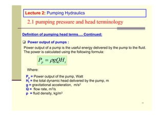
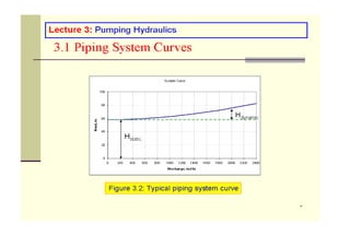
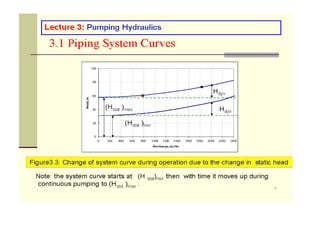
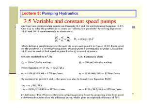
- Key pumping terminology is defined, including static head, total dynamic head (TDH), gage head, velocity head, and friction and minor losses. Pump efficiency and power output equations are also presented.