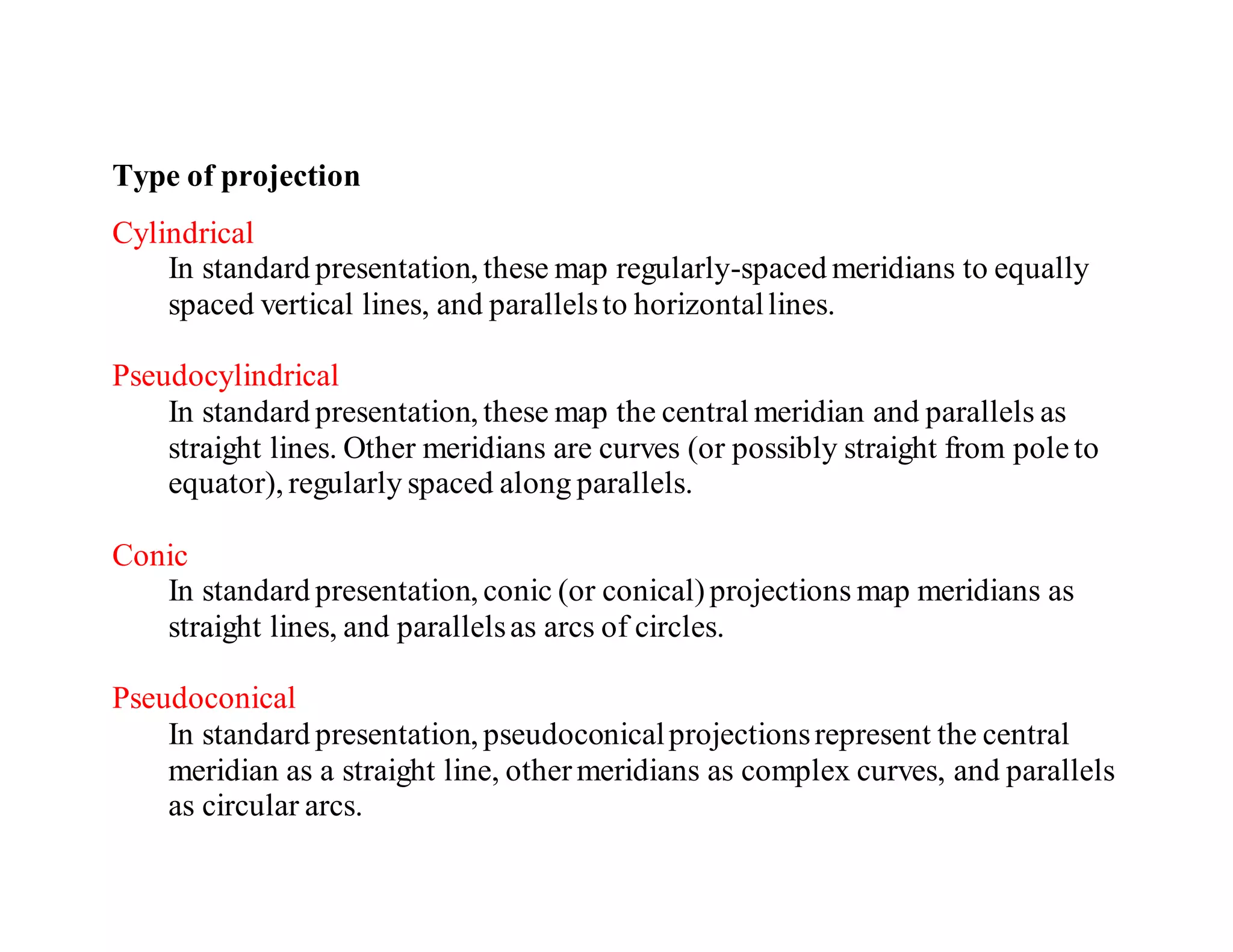
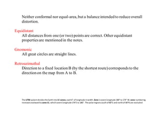
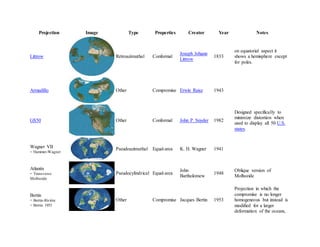
The document describes various types of map projections, including their standard presentations and key properties. It provides examples of specific projections like Mercator, UTM, and Mollweide and notes their creators and intended uses. Tables give more details on individual projections like their image type, properties preserved, year created, and brief descriptions.

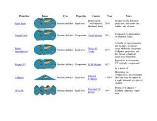
![Projection Image Type Properties Creator Year Notes
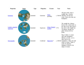
Eckert IV Pseudocylindrical Equal-area
Max Eckert-
Greifendorff
1906
Parallels are unequal in
spacing and scale; outer
meridians are semicircles;
other meridians are
semiellipses.
Eckert VI Pseudocylindrical Equal-area
Max Eckert-
Greifendorff
1906
Parallels are unequal in
spacing and scale; meridians
are half-period sinusoids.
Ortelius oval Pseudocylindrical Compromise Battista Agnese 1540 Meridians are circular.[2]
Goode homolosine Pseudocylindrical Equal-area
John Paul
Goode
1923
Hybrid of Sinusoidal and
Mollweide projections.
Usually used in interrupted
form.
Kavrayskiy VII Pseudocylindrical Compromise
Vladimir V.
Kavrayskiy
1939
Evenly spaced parallels.
Equivalent to Wagner VI
horizontally compressed by
a factor of .
Robinson Pseudocylindrical Compromise
Arthur H.
Robinson
1963
Computed by interpolation
of tabulated values. Used by
Rand McNally since
inception and used by NGS
in 1988–1998.](https://image.slidesharecdn.com/projections-220723042317-98d0816b/85/projections-docx-12-320.jpg)
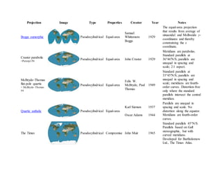
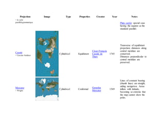
![Projection Image Type Properties Creator Year Notes
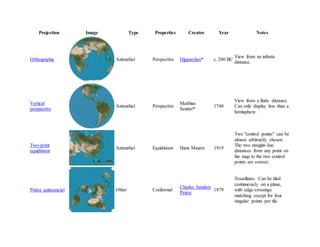
Van der Grinten Other Compromise
Alphons J. van
der Grinten
1904
Boundary is a circle. All
parallels and meridians are
circular arcs. Usually
clipped near 80°N/S.
Standard world projection
of the NGS in 1922–1988.
Equidistant conic
= simple conic
Conic Equidistant
Based on
Ptolemy's 1st
Projection
c. 100
Distances along meridians
are conserved, as is distance
along one or two standard
parallels.[3]
Lambert conformal
conic
Conic Conformal
Johann Heinrich
Lambert
1772 Used in aviation charts.
Albers conic Conic Equal-area
Heinrich C.
Albers
1805
Two standard parallels with
low distortion between
them.](https://image.slidesharecdn.com/projections-220723042317-98d0816b/85/projections-docx-16-320.jpg)
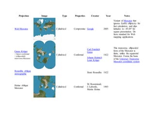
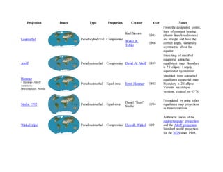
![Projection Image Type Properties Creator Year Notes
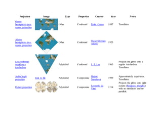
Rectangular
polyconic
Pseudoconical Compromise
U.S. Coast
Survey
c. 1853
Latitude along which scale
is correct can be chosen.
Parallels meet meridians at
right angles.
Latitudinally
equal-differential
polyconic
Pseudoconical Compromise
China State
Bureau of
Surveying and
Mapping
1963
Polyconic: parallels are non-
concentric arcs of circles.
Nicolosi globular Pseudoconical[4] Compromise
Abū Rayḥān al-
Bīrūnī;
reinvented by
Giovanni
Battista
Nicolosi,
1660.[1]:14
c. 1000
Azimuthal
equidistant
=Postel
=zenithal equidistant
Azimuthal Equidistant
Abū Rayḥān al-
Bīrūnī
c. 1000
Distances from center are
conserved.
Used as the emblem of the
United Nations, extending
to 60° S.](https://image.slidesharecdn.com/projections-220723042317-98d0816b/85/projections-docx-18-320.jpg)
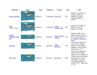
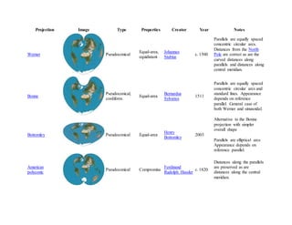
![Projection Image Type Properties Creator Year Notes
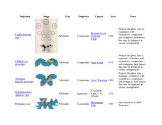
Myriahedral
projections
Polyhedral Equal-area
Jarke J. van
Wijk
2008
Projects the globe onto a
myriahedron: a polyhedron
with a very large number of
faces.[5][6]
Craig
retroazimuthal
= Mecca
Retroazimuthal Compromise
James Ireland
Craig
1909
Hammer
retroazimuthal,
front hemisphere
Retroazimuthal Ernst Hammer 1910
Hammer
retroazimuthal,
back hemisphere
Retroazimuthal Ernst Hammer 1910](https://image.slidesharecdn.com/projections-220723042317-98d0816b/85/projections-docx-23-320.jpg)
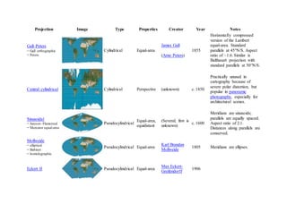
![Projection Image Type Properties Creator Year Notes
to achieve lesser
deformation of the
continents. Commonly used
for French geopolitical
maps.[7]
*The first known popularizer/user and not necessarily the creator.](https://image.slidesharecdn.com/projections-220723042317-98d0816b/85/projections-docx-25-320.jpg)