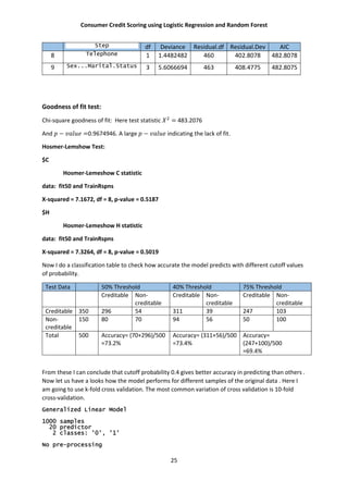
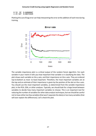
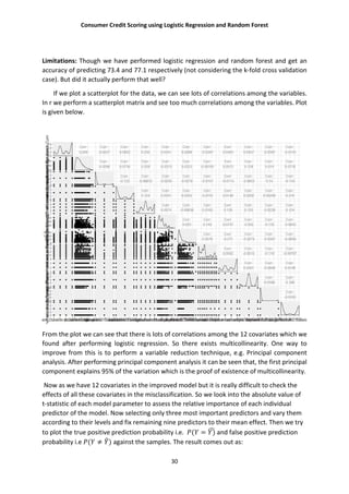
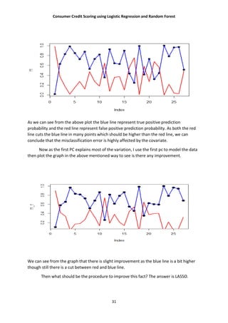
The document discusses using logistic regression and random forest models for consumer credit scoring. It begins by introducing credit scoring and explaining that the goal is to classify applicants as "good" or "bad" credit risks. It then outlines the typical steps taken in developing a credit scoring model, including understanding the problem, defining variables, exploratory data analysis, and splitting data into training and test sets. The document focuses on logistic regression, explaining the logistic regression model and how it is fitted. It also briefly introduces random forest methods and LASSO regularization.
Credit risks are calculated based on the borrowers’ overall ability to repay. Our objective was to use optimization in order to create a tool that approves or rejects loans to borrowers. We also used optimization to establish how much interest rate/credit will be extended to borrowers who were approved for a loan.
Default credit cards are an important issue that bring negative consequences to both sides, i.e, banks and customer. If a customer does not pay his obligations, banks loose money, the customer will lose credibility in future payments, collection calls start to be made and in last resort, the case may go into the court. In order to avoid all of that trouble, effective methods that are able to predict the default of credit cards are needed. Therefore, default credit card prediction is an important, challenging and useful task that should be addressed.
This presentation documents how the problem can be addressed, following the pipeline of a typical Patter Recognition application. The main task is to classify a set of samples representing the history of payments and bill statements of a given client plus some background information about the client according to its ability to pay or not (Default) the next monthly payment of its credit card.
Predicting Credit Card Defaults using Machine Learning AlgorithmsSagar Tupkar
This is a project that I worked on as a Capstone for my Masters in Business Analytics program at the University of Cincinnati. In this project, I have performed an end-to-end data mining exercise including data cleaning, distribution analysis, exploratory data analysis, model building etc. to identify and predict Credit Card defaults using Customer's data on past payments and general profile. In the process for building Machine Learning models, I have fit and compared the performance of multiple models and algorithms like Logistic Regreesion, PCA, Classification tree, AdaBoost Classifier, ANN and LDA.
QU Speaker Series - Session 3
https://qusummerschool.splashthat.com
A conversation with Quants, Thinkers and Innovators all challenged to innovate in turbulent times!
Join QuantUniversity for a complimentary summer speaker series where you will hear from Quants, innovators, startups and Fintech experts on various topics in Quant Investing, Machine Learning, Optimization, Fintech, AI etc.
Topic: Machine Learning and Model Risk (With a focus on Neural Network Models)
All models are wrong and when they are wrong they create financial or non-financial risks. Understanding, testing and managing model failures are the key focus of model risk management particularly model validation.
For machine learning models, particular attention is made on how to manage model fairness, explainability, robustness and change control. In this presentation, I will focus the discussion on machine learning explainability and robustness. Explainability is critical to evaluate conceptual soundness of models particularly for the applications in highly regulated institutions such as banks. There are many explainability tools available and my focus in this talk is how to develop fundamentally interpretable models.
Neural networks (including Deep Learning), with proper architectural choice, can be made to be highly interpretable models. Since models in production will be subjected to dynamically changing environments, testing and choosing robust models against changes are critical, an aspect that has been neglected in AutoML.
Machine Learning Project - Default credit card clients Vatsal N Shah
- The model we built here will use all possible factors to predict data on customers to find who are defaulters and non‐defaulters next month.
- The goal is to find the whether the clients are able to pay their next month credit amount.
- Identify some potential customers for the bank who can settle their credit balance.
- To determine if their customers could make the credit card payments on‐time.
- Default is the failure to pay interest or principal on a loan or credit card payment.
What is Predictive Analytics?
Predictive Analytics is the stream of the advanced analytics which utilizes diverse techniques like data mining, predictive modelling, statistics, machine learning and artificial intelligence to analyse current data and predict future.
To Know more: https://goo.gl/zAcnCR
LOAN DEFAULT PREDICTION – A CASE STUDY
Content Covered in this video:
Business Problem & Benefits
The Risk - LOAN DEFAULT PREDICTION
Data Analysis Process
Data Processing
Predictive Analysis Process
Tools & Technology
AI powered Decision Making in Banks - How Banks today are using Advanced analytics in credit Decisioning, enhancing customer life time value, lower operating costs and stronger customer acquisition
Certain Cases of Customers default on Payments in Taiwan.
From a Risk Management Perspective a Bank/Credit Card Company is more interested in minimizing their losses towards a particular customer.
The information that is more valuable to them is estimating the probability of default rather than classifying a customer as credible/not credible.
Goal: To compute the predictive accuracy of probability of default for a Taiwanese Credit Card Client.
Problem Analysis – Classify Probability of default for next month: 1 as “Default” and 0 as “Not Default”.
Our latest analysis of readiness and maturity of intraday liquidity management shows that many financial institutions run the risk not to meet payment and settlement obligations, if they don’t manage their intraday liquidity effectively. There are ways to make up for the necessary investments to that end by optimizing the intraday liquidity management.
Credit scoring has been used to categorize customers based on various characteristics to evaluate their credit worthiness. Increasingly, machine learning techniques are being deployed for customer segmentation, classification and scoring. In this talk, we will discuss various machine learning techniques that can be used for credit risk applications. Through a case study built in R, we will illustrate the nuances of working with practical data sets which includes categorical and numerical data, different techniques that can be used to evaluate and explore customer profiles, visualizing high dimensional data sets and machine learning techniques for customer segmentation.
Measuring and Managing Credit Risk With Machine Learning and Artificial Intel...accenture
In recent years, technological developments have undergone in-depth analysis among banks, but we are still far from attaining mature levels both at the methodological and at the credit granting, monitoring and control process levels. Banks should equip themselves with new and more structured Model Risk frameworks to manage new Machine Learning model validation paradigms. Learn more from Accenture Finance & Risk: https://accntu.re/2qGUUMx
Credit Scores: What's New
Tuesday, May 3, 11 a.m.-12:30 p.m. ET
This 90-minute webinar will present findings from Experian Public Education Director Rod Griffin and Dr. Barbara O'Neill. This webinar will cover the fundamentals of credit reporting and credit scoring and what you must do to get the credit you want and need.
Speakers: Dr. Barbara O'Neill and Rod Griffin
Register, join & find supporting resources: https://learn.extension.org/events/2488
Improve Your Regression with CART and RandomForestsSalford Systems
Why You Should Watch: Learn the fundamentals of tree-based machine learning algorithms and how to easily fine tune and improve your Random Forest regression models.
Abstract: In this webinar we'll introduce you to two tree-based machine learning algorithms, CART® decision trees and RandomForests®. We will discuss the advantages of tree based techniques including their ability to automatically handle variable selection, variable interactions, nonlinear relationships, outliers, and missing values. We'll explore the CART algorithm, bootstrap sampling, and the Random Forest algorithm (all with animations) and compare their predictive performance using a real world dataset.
Introduction to Analytics
Introduction to SAS
Introduction to Satistics
Introduction to Predictive Modeling
Introduction to Forecasting
Introduction to Bigdata
First presented at the MSUG Conference on June 4, 2015, this presentation discusses concepts and tools to add to your logistic regression modeling practice and also how to use these concepts and tools.
Dr. Trevor Hastie: Data Science of GBM (October 10, 2013: Presented With H2O)Sri Ambati
Dr. Trevor Hastie of Stanford University discusses the data science behind Gradient Boosted Regression and Classification
- Powered by the open source machine learning software H2O.ai. Contributors welcome at: https://github.com/h2oai
- To view videos on H2O open source machine learning software, go to: https://www.youtube.com/user/0xdata
Tree models with Scikit-Learn: Great models with little assumptionsGilles Louppe
This talk gives an introduction to tree-based methods, both from a theoretical and practical point of view. It covers decision trees, random forests and boosting estimators, along with concrete examples based on Scikit-Learn about how they work, when they work and why they work.
A gentle introduction to 2 classification techniques, as presented by Kriti Puniyani to the NYC Predictive Analytics group (April 14, 2011). To download the file please go here: http://www.meetup.com/NYC-Predictive-Analytics/files/
This slide deck presents an introduction to statistical modeling by Don McCormack of JMP. Don presents at Building Better Models seminars throughout the world. Upcoming complimentary US seminars are listed here: http://jmp.com/about/events/seminars/
Tong is a data scientist in Supstat Inc and also a master students of Data Mining. He has been an active R programmer and developer for 5 years. He is the author of the R package of XGBoost, one of the most popular and contest-winning tools on kaggle.com nowadays.
Agenda:
Introduction of Xgboost
Real World Application
Model Specification
Parameter Introduction
Advanced Features
Kaggle Winning Solution
DEVELOPING PREDICTION MODEL OF LOAN RISK IN BANKS USING DATA MINING mlaij
Nowadays, There are many risks related to bank loans, for the bank and for those who get the loans. The
analysis of risk in bank loans need understanding what is the meaning of risk. In addition, the number of
transactions in banking sector is rapidly growing and huge data volumes are available which represent
the customers behavior and the risks around loan are increased. Data Mining is one of the most motivating
and vital area of research with the aim of extracting information from tremendous amount of accumulated
data sets. In this paper a new model for classifying loan risk in banking sector by using data mining. The
model has been built using data form banking sector to predict the status of loans. Three algorithms have
been used to build the proposed model: j48, bayesNet and naiveBayes. By using Weka application, the
model has been implemented and tested. The results has been discussed and a full comparison between
algorithms was conducted. J48 was selected as best algorithm based on accuracy.
An Analysis of Factors Influencing Customer Creditworthiness in the Banking S...Dr. Amarjeet Singh
This research is based on Bahraini bankers’ perception on the factors influencing customer creditworthiness in the banking sector of Kingdom of Bahrain. We consider that the research was done in the Kingdom of Bahrain which has a growing banking industry. To enhance the whole procedure of the creditworthiness, it is vital for an employer to understand the most important factors influencing customer creditworthiness. The purpose of the study was to investigate the factors influencing customers creditworthiness in the banking industry. The creditworthiness can be assessed through qualitative factors, quantitative factors and risk factors. The research was conducted through a survey, using the questionnaire as the research instrument. The respondents of the study are employees of banks across the Kingdom dealing with creditworthiness. The statistical tools used in the study are Multiple Regression Analyses and weighted mean. The researcher has found that there is significant relationship between all three factors and creditworthiness, and they don’t equally influence the creditworthiness. The research provides recommendations to banks in assessing the creditworthiness. The researcher recommended that employees must use the most effective methods such as credit scoring to conduct the analysis of creditworthiness in order to make effective decisions. Moreover, the researcher recommended that analysts should take into considerations the most effective factors in the analysis process and they must not neglect other.
https://ijitce.com/index.php
Our journal maintains rigorous peer review standards. Each submitted article undergoes a thorough evaluation by experts in the respective field. This stringent review process helps ensure that only high-quality and scientifically sound research is accepted for publication. Researchers can trust that the articles they find in IJITCE have been critically assessed for validity, significance, and originality.
PROBABILISTIC CREDIT SCORING FOR COHORTS OF BORROWERSAndresz26
Este Working Paper relata sobre el nivel del riesgo crediticio, se debe reconocer que el riesgo de un grupo proviene de la diversidad de sus miembros, este libro propone una metodología para la aplicación de la medición del riesgo crediticio, y permite hacer un ranking de la población por su nivel de riesgo. La misma que realiza una distinción en los diferentes rankings de la población por su nivel de riesgo, y considerando en el ranking los riesgos de sus preferencias en sus decisiones realizadas.
http://www.udla.edu.ec/
Running Head BANK LENDING PRACTICES AT THE BANK OF AMERICABANK .docxsusanschei
Running Head: BANK LENDING PRACTICES AT THE BANK OF AMERICA
BANK LENDING PRACTICES AT THE BANK OF AMERICA 4
Bank Lending Practices at the Bank of America
Rasmussen College
March 19, 2017
Individual and Commercial Lending Practices
As one of the largest financial organizations, the Bank of America (BOA) serves both personal and commercial businesses and corporations. Businesses owners are offered loans to enable them to purchase inventory and materials. Furthermore, loans are provided by the BOA to refinance debt or finance account receivables. In the individual aspects, loans on mortgages are given to enable people to fund their new homes. Car loans are also get provided to the client as the banks depending on the eligibility of an individual (Hanken, Young, Smilowitz, Chiampas & Waskowski, 2016).
Under the Small Business Administration Federal Agency, the Bank of America offers loans to small established businesses and to firms that are getting started. A minimum of $350,000 gets provided to businesses to buy equipment or purchasing real estate. The loan can get paid for a seven-year term. Competitive variable rates based on prime rates gets offered. Considerations get made in a type of relationship an individual or business has with the bank. An online banking system is also provided to give clients more access to their finances.
Risk Measurement Techniques
Risk analysis and management are indispensable at the Bank of America in particular with the high rates or credits offered to individuals and commercial corporations. The Bank of America utilizes different strategies for competency credit risk policies to monitor and manage credit risks in the company. A team of credit risk analyst exists that extensive conduct analysis of the bank’s exposure to credit risks. Studies are carried out on financial statements of industrial corporations to determine their credibility for credit. For individual loans, credit-card loss forecasting is done to assess and calculate the risks of personal lending. On the other hand, an SAS Enterprise Risk Management system and an IBM grid are used in to evaluate the risks exposed to the bank. The high technologies can ensure that useful calculations on statistics are conducted to determine the credit risks in the bank. Consequently, almost accurate forecasts can be made therefore evading considerable risks on the part of the company. Short term deposits get required from all borrowers to according to the time frame indicated in the issuance of credit. The Bank of America has a Corporate Investments Group that models and calculates the risks and probability of default to securities offered. Furthermore, a compliance team also exists and provides guidance and advice to the Bank on issues related to financial lending.
Benefits of Transfer of Credit Risk
There are various benefits associated with the transfer of credit risks. One of the most apparent ...
Our goal with this commentary is to put common credit score myths to rest, and to shed some light on what the insights and research from Equifax proves to be true.
WNS’ commercial banking solutions coupled with cutting-edge transformational solutions enable superior customer experience & cost-effective commercial banking operations.
Get more details on - https://s3.wns.com/S3_5/Documents/Articles/PDFFiles/7064/274/3_Step_Changes_That_Transform_Commercial_Credit_Appraisal.pdf
Despite the proliferation of banking services, lending to industry and
the public still constitutes the core of the income of commercial banks and
other lending institutions in developed as well as post-transition countries.
From the technical perspective, the lending process in general is a relatively
straightforward series of actions involving two principal parties. These activities
range from the initial loan application to the successful or unsuccessful
repayment of the loan. Although retail lending belongs among
the most profitable investments in lenders’ asset portfolios (at least in developed
countries), increases in the amounts of loans also bring increases
in the number of defaulted loans, i.e. loans that either are not repaid at all
or cases in which the borrower has problems with paying debts. Thus,
the primary problem of any lender is to differentiate between “good” and
“bad” debtors prior to granting credit. Such differentiation is possible by using
a credit-scoring method. The goal of this paper is to review credit-scoring
methods and elaborate on their efficiency based on the examples from
the applied research. Emphasis is placed on credit scoring related to retail
loans.
AI-based credit scoring - An Overview.pdfStephenAmell4
AI-based credit scoring is a contemporary method for evaluating a borrower’s creditworthiness. In contrast to the conventional approach that hinges on static variables and historical information, AI-based credit scoring harnesses the power of machine learning algorithms to scrutinize an extensive array of data from various sources.
MSc research project report - Optimisation of Credit Rating Process via Machi...AmarnathVenkataraman
Optimization of Credit rating process via Machine Learning
The credit rating process is considered to be one of the vital processes that defenses the global economy. The majority of investments will be obtained based on these credit ratings which acts as the representation of the financial credibility of companies. As the current credit rating process found to be expensive, small and medium-sized enterprises(SMEs) which are considered to be the backbone of the global economy might find it difficult to access the funds via investment for their development which in turn affects the global economy as well. This issue might be solved with the outcome of this research in terms of the optimized credit rating system with improved accuracy and continuous credit rating transition. Support Vector Machine(SVM) managed to achieve the highest accuracy of 92.0% whereas Random Forest(RF) and C5.0 decision tree also achieved greater accuracies with different formats of the dataset. With the help of dictionary-based sentiment analysis, this research proved that a continuous credit rating transition system could track the changes in the financial status of the company which in turn helps to predict the crisis like bankruptcy and default in prior.
Barclays - Case Study Competition | ISB | National FinalistNaveen Kumar
We were the National Finalist in the case study competition organized by ISB partnered with Barclays.
Our solution to Barclay's bank to increase its foray into the consumer lending bank using customer segmentation using clustering techniques - Multi factor cluster analysis on 1.5 Million credit profile datasets.
We identified profitable pools from our ML model which were then coupled with upcoming banking trends such as open banking to increase market share.
Similar to Consumer Credit Scoring Using Logistic Regression and Random Forest (20)
Techniques to optimize the pagerank algorithm usually fall in two categories. One is to try reducing the work per iteration, and the other is to try reducing the number of iterations. These goals are often at odds with one another. Skipping computation on vertices which have already converged has the potential to save iteration time. Skipping in-identical vertices, with the same in-links, helps reduce duplicate computations and thus could help reduce iteration time. Road networks often have chains which can be short-circuited before pagerank computation to improve performance. Final ranks of chain nodes can be easily calculated. This could reduce both the iteration time, and the number of iterations. If a graph has no dangling nodes, pagerank of each strongly connected component can be computed in topological order. This could help reduce the iteration time, no. of iterations, and also enable multi-iteration concurrency in pagerank computation. The combination of all of the above methods is the STICD algorithm. [sticd] For dynamic graphs, unchanged components whose ranks are unaffected can be skipped altogether.
06-04-2024 - NYC Tech Week - Discussion on Vector Databases, Unstructured Data and AI
Round table discussion of vector databases, unstructured data, ai, big data, real-time, robots and Milvus.
A lively discussion with NJ Gen AI Meetup Lead, Prasad and Procure.FYI's Co-Found
Adjusting primitives for graph : SHORT REPORT / NOTESSubhajit Sahu
Graph algorithms, like PageRank Compressed Sparse Row (CSR) is an adjacency-list based graph representation that is
Multiply with different modes (map)
1. Performance of sequential execution based vs OpenMP based vector multiply.
2. Comparing various launch configs for CUDA based vector multiply.
Sum with different storage types (reduce)
1. Performance of vector element sum using float vs bfloat16 as the storage type.
Sum with different modes (reduce)
1. Performance of sequential execution based vs OpenMP based vector element sum.
2. Performance of memcpy vs in-place based CUDA based vector element sum.
3. Comparing various launch configs for CUDA based vector element sum (memcpy).
4. Comparing various launch configs for CUDA based vector element sum (in-place).
Sum with in-place strategies of CUDA mode (reduce)
1. Comparing various launch configs for CUDA based vector element sum (in-place).
Quantitative Data AnalysisReliability Analysis (Cronbach Alpha) Common Method...2023240532
Quantitative data Analysis
Overview
Reliability Analysis (Cronbach Alpha)
Common Method Bias (Harman Single Factor Test)
Frequency Analysis (Demographic)
Descriptive Analysis
Adjusting OpenMP PageRank : SHORT REPORT / NOTESSubhajit Sahu
For massive graphs that fit in RAM, but not in GPU memory, it is possible to take
advantage of a shared memory system with multiple CPUs, each with multiple cores, to
accelerate pagerank computation. If the NUMA architecture of the system is properly taken
into account with good vertex partitioning, the speedup can be significant. To take steps in
this direction, experiments are conducted to implement pagerank in OpenMP using two
different approaches, uniform and hybrid. The uniform approach runs all primitives required
for pagerank in OpenMP mode (with multiple threads). On the other hand, the hybrid
approach runs certain primitives in sequential mode (i.e., sumAt, multiply).
Consumer Credit Scoring Using Logistic Regression and Random Forest
1. Consumer Credit Scoring using Logistic Regression and Random Forest
1
Consumer credit scoring using Logistic
Regression and Random Forest
A DISSERTATION SUBMITTED IN PARTIAL
FULFILLMENT OF THE REQUIREMENTS FOR THE
DEGREE OF MASTER OF SCIENCE IN STATISTICS OF
THE WEST BENGAL STATE UNIVERSITY
HIRAK SEN ROY
REG. NO. 214003129
DEPARTMENT OF STATISTICS
2. Consumer Credit Scoring using Logistic Regression and Random Forest
2
ABSTRACT
Credit scoring has been regarded as a core appraisal tool of different institutions during the
last few decades, and has been widely investigated in different areas, such as finance and
accounting. Different scoring techniques are being used in areas of classification and
prediction, where statistical techniques have conventionally been used. Credit scoring is the
term used to describe formal statistical methods used for classifying applicants into “good”
and “bad” risk classes. Such methods have become increasingly important with the dramatic
growth in consumer credit in recent years. In this study, the concept and application of credit
scoring in a German banking environment is explained. The steps necessary to develop a
credit scoring model is looked at with focus on the credit risk context. The statistics behind
credit scoring is also explained, with particular emphasis on logistic regression. As logistic
regression is not the only method used in credit scoring, a popular non parametric
classification method, random forest will also be discussed. Limitations using logistic
regression will be explained via the effects of covariates in misclassification and possible
solutions will be given mainly using LASSO.
3. Consumer Credit Scoring using Logistic Regression and Random Forest
3
Chapter 1: Introduction
A credit score is a numerical expression based on a statistical analysis of a person's credit files,
to represent the creditworthiness of that person. A credit score is primarily based on credit
report information typically sourced from credit bureaus. Lenders, such as banks and credit
card companies, use credit scores to evaluate the potential risk posed by lending money to
consumers and to mitigate losses due to bad debt. Lenders use credit scores to determine
who qualifies for a loan, at what interest rate, and what credit limits. Lenders also use credit
scores to determine which customers are likely to bring in the most revenue. At the same
time, credit scoring is not limited to banks. Other organizations, such as mobile phone
companies, insurance companies, landlords, and government departments employ the same
techniques.
Here we have the credit information of 1000 German individuals from pre-euro
era. They applied for bank loan for various purposes. Some of the individuals defaulted after
certain period. The bank wants to create a decision support system to help the loan officer
using this data.
When a bank receives a loan application, based on the applicant’s profile the bank
has to make a decision regarding whether to go ahead with the loan approval or not. Two
types of risks are associated with the bank’s decision –
If the applicant is a good credit risk, i.e. is likely to repay the loan, then not approving the
loan to the person results in a loss of business to the bank
If the applicant is a bad credit risk, i.e. is not likely to repay the loan, then approving the
loan to the person results in a financial loss to the bank
Our objective of analysis here is – “Minimization of risk and maximization of profit on behalf
of the bank.”
To minimize loss from the bank’s perspective, the bank needs a decision rule regarding who to
give approval of the loan and who not to. An applicant’s demographic and socio-economic profiles
are considered by loan managers before a decision is taken regarding his/her loan application.
1.1 Brief Outline of the Study
In the second chapter a brief history of credit and subsequent modern development in credit
scoring model will be outlined. Some benefits and criticisms will be given,
Chapter three discusses steps in credit scoring model development.
Chapter four discusses in detail the logistic regression model, interpretation of
a fitted logistic model, model building strategies, assessing the fit of the model.
Chapter five gives a brief outline of random forest methods and how it can be
used in credit scoring. Chapter six gives a brief overview of LASSO (least absolute shrinkage
and selection operator).
4. Consumer Credit Scoring using Logistic Regression and Random Forest
4
In chapter seven data analysis based on the German credit scoring data will be
shown. Results will be outlined and necessary comments will be given.
Appendix section covers the codes used for the analysis and a brief description
of the data set.
5. Consumer Credit Scoring using Logistic Regression and Random Forest
5
Chapter 2: Credit Scoring
2.1 Historical Motivation
The phenomenon of borrowing and lending has a long history associated with human
behaviour (Thomas et al., 2002). Therefore, credit is perhaps a phenomenon as old as trade
and commerce. Despite the very long history of credit back to around 2000 BC or earlier, the
history of credit scoring is very short, beginning only about six decades ago. Information
collected by banks and/or financial institutions of a credit applicant is used to develop a
numerical score for each applicant (Thomas et al., 2002; Hand & Jacka, 1998; Lewis, 1992).
Recently, credit scoring techniques have been expanded to include more applications in
different fields. Moreover, the idea of reducing the probability of a customer defaulting,
which predicts customer risk, is a new role for credit scoring, which can support and help
maximize the expected profit from that customer for financial institutions, especially banks.
By the start of the 21st century, the use of credit scoring had expanded more and more,
especially with the tremendous technologies created, introducing more advanced techniques
and evaluation criteria, such as GINI and area under the ROC curve. Besides, the high
capabilities of computing technology make the use of credit scoring much easier than before.
2.2 Credit Scoring Definitions
Credit evaluation is one of the most crucial processes in banks’ credit management decisions.
This process includes collecting, analysing and classifying different credit elements and
variables to assess the credit decisions. The quality of bank loans is the key determinant of
competition, survival and profitability. One of the most important kits, to classify a bank’s
customers, as a part of the credit evaluation process to reduce the current and the expected
risk of a customer being bad credit, is credit scoring. Hand & Jacka, (1998, p. 106) stated that
“the process (by financial institutions) of modelling creditworthiness is referred to as credit
scoring”. It is also useful to provide further definitions of credit scoring.
Credit scoring models (see, for example: Lewis, 1992; Bailey, 2001; Mays, 2001; Malhotra &
Malhotra, 2003; Thomas et al., 2004; Sidique, 2006; Chuang & Lin, 2009; Sustersic et al, 2009)
are some of the most successful applications of research modelling in finance and banking, as
reflected in the number of scoring analysts in the industry, which is continually increasing.
“However, credit scoring has been (vital) in allowing the phenomenal growth in consumer
credit over the last five decades. Without (credit scoring techniques, as) an accurate and
automatically operated risk assessment tool, lenders of consumer credit could not have
expanded their loan (effectively)” (Thomas et al, 2002, p. xiii).
6. Consumer Credit Scoring using Logistic Regression and Random Forest
6
2.3 Benefits and Criticisms of Credit Scoring
Benefits of credit scoring: credit scoring requires less information to make a decision, because
credit scoring models have been estimated to include only those variables, which are
statistically and/or significantly correlated with repayment performance; whereas
judgemental decisions, prima facie, have no statistical significance and thus no variable
reduction methods are available (Crook, 1996). Credit scoring models attempt to correct the
bias that would result from considering the repayment histories of only accepted applications
and not all applications. They do this by assuming how rejected applications would have
performed if they had been accepted. Judgemental methods are usually based on only the
characteristics of those who were accepted, and who subsequently defaulted (Crook, 1996).
Credit scoring models consider the characteristics of good as well as bad payers, while,
judgemental methods are generally biased towards awareness of bad payers only. Credit
scoring models are built on much larger samples than a loan analyst can remember. Credit
scoring models can be seen to include explicitly only legally acceptable variables whereas it is
not so easy to ensure that such variables are ignored by a loan analyst. Credit scoring models
demonstrate the correlation between the variables included and repayment behaviour,
whereas this correlation cannot be demonstrated in the case of judgemental methods
because many of the characteristics which a loan analyst may use are not impartially
measured. A credit scoring model includes a large number of a customer’s characteristics
simultaneously, including their interactions, while a loan analyst’s mind cannot arguably do
this, for the task is too challenging and complex. An additional essential benefit of credit
scoring is that the same data can be analysed easily and clearly by different credit analysts or
statisticians and give the same weights. This is highly unlikely to be so in the case of
judgemental methods (Chandler & Coffman, 1979; Crook, 1996).
Criticisms of credit scoring: credit scores use any characteristic of a customer in spite of
whether a clear link with a likely repayment can be justified. Also, sometimes economic
factors are not included. In addition, using credit scoring models, sometimes customers may
have the characteristics, which make them more similar too bad than good payers, but may
have these entirely by chance (a misclassification problem). Statistically a credit scoring model
is “incomplete”, for it leaves out some variables, which taken with the others, might predict
that the customer will repay. But unless a credit scoring model has every possible variable in
it, normally it will misclassify some people. Another criticism of credit scoring models is the
possibility of indirect discrimination (Crook, 1996). Furthermore, credit scoring models: are
not standardized and differ from one market to another; are expensive to buy and
subsequently to train credit analysts; and sometimes a credit scoring system may “reject (a)
creditworthy applicant because he/she changes address or job‟ (Al Amari, 2002, p. 69; citing
Chandler & Coffman, 1979).
7. Consumer Credit Scoring using Logistic Regression and Random Forest
7
Chapter 3: Steps in Credit Scoring Model
Development
Credit scoring is a mechanism used to quantify the risk factors relevant for an obligor’s ability
and willingness to pay. The aim of the credit score model is to build a single aggregate risk
indicator for a set of risk factors. The risk indicator indicates the ordinal or cardinal credit risk
level of the obligor. To obtain this, several issues needs to be addressed, and is explained in
the following steps:
3.1 Understanding the business problem
The aim of the model should be determined in this step. It should be clear what this model
will be used for as this influences the decisions of which technique to use and what
independent variables will be appropriate. It will also influence the choice of the dependent
variable.
3.2 Defining the dependent variable
The definition identifies events vs. non-events (0- 1 dependent variable). In the credit scoring
environment, one will mostly focus on the prediction of default. Note that an event (default)
is normally referred to as a "bad" and a non -event as a "good".
Note that the dependent variable will also be referred to as either the outcome or
in traditional credit scoring the "bad" or default variable. In credit scoring, the default
definition is used to describe the dependent (outcome) variable. In our dataset the dependent
variable is defined as “Creditability”.
3.3 Exploratory Data Analysis
There exist several methods for quickly producing and visualizing simple summaries of data
sets (Tukey,1977). Exploratory data analysis or “EDA” is a critical first step in analysing the
data from an experiment. Here are the main reasons we use EDA:
detection of mistakes
checking of assumptions
preliminary selection of appropriate models
determining relationships among the explanatory variables, and
assessing the direction and rough size of relationships between explanatory
and outcome variables.
Loosely speaking, any method of looking at data that does not include formal statistical
modeling and inference falls under the term exploratory data analysis.
8. Consumer Credit Scoring using Logistic Regression and Random Forest
8
Exploratory data analysis is generally cross-classified in two ways. First, each method
is either non-graphical or graphical. And second, each method is either univariate or
multivariate.
Non-graphical methods generally involve calculation of summary statistics, while
graphical methods obviously summarize the data in a diagrammatic or pictorial way.
Univariate methods lo ok at one variable (data column) at a time, while multivariate methods
look at two or more variables at a time to explore relationships. It is almost always a good
idea to perform univariate EDA on each of the components of a multivariate EDA before
performing the multivariate EDA.
3.3 Splitting the datasets
When our objective turns to prediction, and in particular towards the development of
predictive models, we will typically use our models to guide many decisions, and to make
hundreds, thousands, or even billions of predictions. With a predictive model our principal
focus is no longer on the data but on a type of theory about reality.
The simplest partition possible for cross-sectional data is a two-way random partition to
generate a learning (or training) set and a test set (sometimes instead referred to as a
validation set). The thinking underlying such a division is that:
The data available for analytics fairly represents the real world processes we wish to
model
The real world processes we wish to model are expected to remain relatively stable
over time so that a well-constructed model built on last month’s data is reasonably
expected to perform adequately on next month’s data
Why Bother Creating a test partition?
First and foremost, we create test partitions to provide us honest assessments of the
performance of our predictive models. No amount of mathematical reasoning and
manipulation of results based on the training data will be convincing to an experienced
observer. Most of us have encountered strategies for profitable stock selection that
perform brilliantly on past (training) data but somehow fall down where it counts,
namely on future data. The same will apply to any predictive model we generate with
modern learning machines.
9. Consumer Credit Scoring using Logistic Regression and Random Forest
9
Chapter 4: Logistic Regression
4.1 Introduction:
What distinguishes a logistic regression model from the linear regression model is that the
outcome variable in logistic regression is binary or dichotomous. This difference between
logistic and linear regression is reflected both in the form of the model and its assumptions.
Once this difference is accounted for, the methods employed in an analysis using logistic
regression follow, more or less, the same general principles used in linear regression. Thus,
the techniques used in linear regression analysis motivate our approach to logistic regression.
4.2 The principles behind logistic regression:
In simple linear regression, we saw that the outcome variable Y is predicted from the equation
of a straight line: ( | ) = + in which is the intercept and is the slope of the
straight line, is the value of the predictor variable. In multiple regression, in which there are
several predictors, a similar equation is derived in which each predictor has its own
coefficient. In logistic regression, instead of predicting the value of a variable Y from predictor
variables, we calculate the probability of = Yes given known values of the predictors. The
logistic regression equation bears many similarities to the linear regression equation. In its
simplest form, when there is only one predictor variable, the logistic regression equation from
which the probability of Y is predicted is given by:
1
1 + ( )
One of the assumptions of linear regression is that the relationship between variables is
linear. When the outcome variable is dichotomous, this assumption is usually violated. The
logistic regression equation described above expresses the multiple linear regression
equation in logarithmic terms and thus overcomes the problem of violating the assumption
of linearity. On the hand, the resulting value from the equation is a probability value that
varies between 0 and 1. A value close to 0 means that is very unlikely to have occurred, and
a value close to 1 means that Y is very likely to have occurred.
4.3 Logistic regression model:
Usually, binary data result from a nonlinear relationship between ( ) = ( | ) and . A
fixed change in often has less impact when ( ) is near 0 or 1 than when ( ) is near 0.5.
In practice, nonlinear relationships between ( ) and are often monotonic, with ( )
increasing continuously or ( ) decreasing continuously as increases. The S-shaped curves
in Figure 4.1 are typical. The most important curve with this shape has the model formula
( ) =
exp( + )
1 + exp( + )
10. Consumer Credit Scoring using Logistic Regression and Random Forest
10
This is the logistic regression model. As → ∞, ( ) ↓ 0 when < 0 and ( ) ↑ 1 when
> 0.
The odds are
( )
( )
= exp( + ). The log odds called the logit has the linear
relationship:
( ) = log
( )
( )
= + .
The curve in the above is defined by the equation ( ) =
( )
( )
. We can see that it
is S-shaped.
4.4 Fitting the logistic regression model:
Suppose we have a s ample of n independent observations of the pair ( , ), = 1, 2, ..., n,
where denotes the value of a dichotomous outcome variable and is the value of the
independent variable for the th subject. Furthermore, assume that the outcome variable has
been coded as 0 or 1, representing the absence or the presence of the characteristic,
respectively. This coding for a dichotomous outcome is used throughout the text. Fitting the
logistic regression model in equation to a set of data requires that we estimate the values
of 0
, 1
, the unknown parameters.
To fit a logistic regression model ( ) =
exp 0+ 1
1+exp( 0+ 1 )
to a set of data requires
that the value of 0
, 1
to be estimated. Now with some models, like the logistic curve, there is
no mathematical solution that will produce explicit expressions for least square estimates of
11. Consumer Credit Scoring using Logistic Regression and Random Forest
11
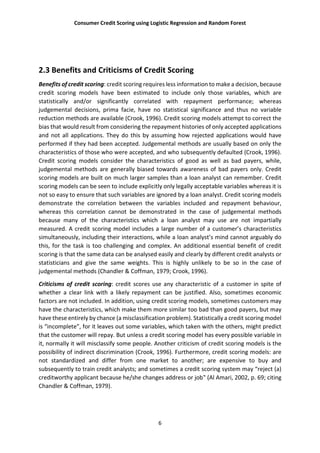
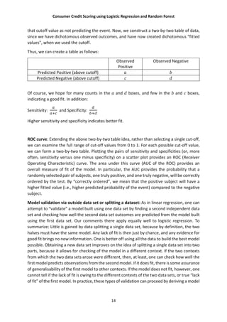
the parameters. The approach that will be followed here is called maximum likelihood. This
method yields values for the unknown parameters that maximize the probability of obtaining
the observed set of data. To apply this method, a likelihood function must be constructed.
This function expressed the probability of the observed data as a function of the unknown
parameters. The maximum likelihood estimators of these parameters are chosen that this
function is maximized, hence the resulting estimators will agree most closely with the
observed data.
Now if is coded as 0 or 1, the expression for ( ) =
( )
( )
provides
conditional probability that = 1 given . This is denoted as ( ). It follow that 1 − ( ) gives the
conditional probability that = 1 given . Now this can be expressed for the observation ( , ) as:
( ) [1 − ( )]
The assumption is that the observations are independent, thus the likelihood function is
obtained as a product of the terms given by the above expression.
(β) = ∏( ( ) [1 − ( )] )
Where is the vector of unknown parameters.
Now has to be estimated so that (β) is maximized. The log likelihood
function is defined as:
( ) = { ln[ ( )] + (1 − ) ln[1 − ( )]}.
In linear regression, the normal equations obtained by minimizing the SSE, was linear in the
unknown parameters that are easily solved. In logistic regression, minimizing the log
likelihood yields equations that are nonlinear in the unknowns, so numerical methods are
used to obtain their solutions.
Deviance: Compare the observed values of the response variable to predicted values
obtained from models with and without the variable in question. In logistic regression,
comparison of observed to predicted values is based on the log likelihood function.
To better understand this comparison, it is helpful conceptually to think of an
observed value of the response variable as also being a predicted value resulting from a
saturated model. A saturated model is one that contains as many parameters as there are
data points.
The comparison of the observed to predicted values using the likelihood
function is based on the following expression:
= −2 ln
ℎ ( )
ℎ ( )
Substituting the likelihood function gives us the deviance statistic:
= −2 ∑ ln + (1 − ) ln .
12. Consumer Credit Scoring using Logistic Regression and Random Forest
12
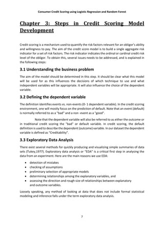
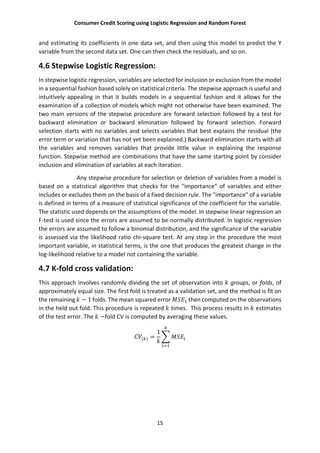
Likelihood Ratio Test: The likelihood-ratio test uses the ratio of the maximized value of the
likelihood function for the full model ( ) over the maximized value of the likelihood function
for the simpler model ( ). The full model has all the parameters of interest in it. The
likelihood ratio test statistic equals:
−2 ln = −2[ln − ln ]
The likelihood-ratio test tests if the logistic regression coefficient for the dropped
variable can be treated as zero, thereby justifying the dropping of the variable from the
model.
Wald Test: The Wald test is used to test the statistical significance of each coefficient ( ) in
the model. A Wald test calculates a statistic which is:
=
This value is squared which yields a chi-square distribution and is used as the Wald
test statistic. (Alternatively the value can be directly compared to a normal distribution.)
Score Test: A test for significance of a variable, which does not require the computation of
the maximum likelihood estimates for the coefficients, is the Score test. The Score test is
based on the distribution of the derivatives of the log likelihood.
Let be the likelihood function which depends on a univariate parameter and let
be the data. The score is ( ) where
( ) =
ln ( | )
The observed Fisher information is
( ) =
ln ( | )
The statistic to test : = is: ( ) =
( )
( )
Which take (1) distribution asymptotically when is true.
4.5 Goodness of fit in Logistic regression
As in linear regression, goodness of fit in logistic regression attempts to get at how well a
model fits the data. It is usually applied after a “final model” has been selected. As we have
seen, often in selecting a model no single “final model” is selected, as a series of models are
fit, each contributing towards final inferences and conclusions. In that case, one may wish to
see how well more than one model fits, although it is common to just check the fit of one
13. Consumer Credit Scoring using Logistic Regression and Random Forest
13
model. This is not necessarily bad practice, because if there are a series of “good” models
being fit, often the fit from each will be similar.
The following measures of fit are available, sometimes divided into “global” and “local”
measures:
Chi-square goodness of fit tests and deviance
Hosmer-Lemshow Tests
Classification Tables
ROC curves
Logistic regression
Model validation via outside data set or by splitting the data set
Chi-square Test: Define standardize residual as
=
−
−
One can find statistics as
=
The statistics follows distribution with − ( + 1) degrees of freedom.
Hosmer-Lemshow Test: The Hosmer-Lemeshow goodness of fit test is based on dividing the
sample up according to their predicted probabilities, or risks. Specifically, based on the
estimated parameter values for each observation in the sample the probability that = 1
is calculated, based on each observation's covariate values: consider fitting a logistic
regression model, calculating all fitted values and grouping the covariate patterns
according to the ordering of from lowest to highest, say. The test statistic can be defined
as
( − )
Provided ( + 1) < . Where denotes the number of observed = 0 in the group
denotes the number of observed = 1 in the group and and denotes the
number of zeroes.
Classification tables: In an idea similar to that above, one can again start by fitting a model
and calculating all fitted values. Then, one can choose a cutoff value on the probability scale,
say 50%, and classify all predicted values above that as predicting an event, and all below
14. Consumer Credit Scoring using Logistic Regression and Random Forest
14
that cutoff value as not predicting the event. Now, we construct a two-by-two table of data,
since we have dichotomous observed outcomes, and have now created dichotomous “fitted
values”, when we used the cutoff.
Thus, we can create a table as follows:
Observed
Positive
Observed Negative
Predicted Positive (above cutoff)
Predicted Negative (above cutoff)
Of course, we hope for many counts in the and boxes, and few in the and boxes,
indicating a good fit. In addition:
Sensitivity: and Specificity:
Higher sensitivity and specificity indicates better fit.
ROC curve: Extending the above two-by-two table idea, rather than selecting a single cut-off,
we can examine the full range of cut-off values from 0 to 1. For each possible cut-off value,
we can form a two-by-two table. Plotting the pairs of sensitivity and specificities (or, more
often, sensitivity versus one minus specificity) on a scatter plot provides an ROC (Receiver
Operating Characteristic) curve. The area under this curve (AUC of the ROC) provides an
overall measure of fit of the model. In particular, the AUC provides the probability that a
randomly selected pair of subjects, one truly positive, and one truly negative, will be correctly
ordered by the test. By “correctly ordered”, we mean that the positive subject will have a
higher fitted value (i.e., higher predicted probability of the event) compared to the negative
subject.
Model validation via outside data set or splitting a dataset: As in linear regression, one can
attempt to “validate” a model built using one data set by finding a second independent data
set and checking how well the second data set outcomes are predicted from the model built
using the first data set. Our comments there apply equally well to logistic regression. To
summarize: Little is gained by data splitting a single data set, because by definition, the two
halves must have the same model. Any lack of fit is then just by chance, and any evidence for
good fit brings no new information. One is better off using all the data to build the best model
possible. Obtaining a new data set improves on the idea of splitting a single data set into two
parts, because it allows for checking of the model in a different context. If the two contexts
from which the two data sets arose were different, then, at least, one can check how well the
first model predicts observations from the second model. If it does fit, there is some assurance
of generalisability of the first model to other contexts. If the model does not fit, however, one
cannot tell if the lack of fit is owing to the different contexts of the two data sets, or true “lack
of fit” of the first model. In practice, these types of validation can proceed by deriving a model
15. Consumer Credit Scoring using Logistic Regression and Random Forest
15
and estimating its coefficients in one data set, and then using this model to predict the Y
variable from the second data set. One can then check the residuals, and so on.
4.6 Stepwise Logistic Regression:
In stepwise logistic regression, variables are selected for inclusion or exclusion from the model
in a sequential fashion based solely on statistical criteria. The stepwise approach is useful and
intuitively appealing in that it builds models in a sequential fashion and it allows for the
examination of a collection of models which might not otherwise have been examined. The
two main versions of the stepwise procedure are forward selection followed by a test for
backward elimination or backward elimination followed by forward selection. Forward
selection starts with no variables and selects variables that best explains the residual (the
error term or variation that has not yet been explained.) Backward elimination starts with all
the variables and removes variables that provide little value in explaining the response
function. Stepwise method are combinations that have the same starting point by consider
inclusion and elimination of variables at each iteration.
Any stepwise procedure for selection or deletion of variables from a model is
based on a statistical algorithm that checks for the "importance" of variables and either
includes or excludes them on the basis of a fixed decision rule. The "importance" of a variable
is defined in terms of a measure of statistical significance of the coefficient for the variable.
The statistic used depends on the assumptions of the model. In stepwise linear regression an
F-test is used since the errors are assumed to be normally distributed. In logistic regression
the errors are assumed to follow a binomial distribution, and the significance of the variable
is assessed via the likelihood ratio chi-square test. At any step in the procedure the most
important variable, in statistical terms, is the one that produces the greatest change in the
log-likelihood relative to a model not containing the variable.
4.7 K-fold cross validation:
This approach involves randomly dividing the set of observation into groups, or folds, of
approximately equal size. The first fold is treated as a validation set, and the method is fit on
the remaining − 1 folds. The mean squared error then computed on the observations
in the held out fold. This procedure is repeated times. This process results in estimates
of the test error. The −fold CV is computed by averaging these values.
( ) =
1
16. Consumer Credit Scoring using Logistic Regression and Random Forest
16
Chapter 5: Random Forest
5.1 An Overview of classification:
The linear regression model assumes that the response variable is quantitative. But in many
situations, the response variable is instead qualitative. For example, eye colour is qualitative,
taking on values blue, brown, or green. Often qualitative variables are referred to as
categorical; we will use these terms interchangeably. In this chapter, we study approaches for
predicting qualitative responses, a process that is known as classification. Predicting a
qualitative response for an observation can be referred to as classifying that observation,
since it involves assigning the observation to a category, or class. On the other hand, often
the methods used for classification first predict the probability of each of the categories of a
qualitative variable, as the basis for making the classification. In this sense they also behave
like regression methods.
Models of data with a categorical response are called classifiers. A classifier is
built from training data, for which classifications are known. The classifier assigns new test
data to one of the categorical levels of the response. Previously we have discussed one of the
most widely used classifier: Logistic regression.
5.2 Introduction to random forest:
To take advantage of the sheer size of modern data sets, we now need learning algorithms
that scale with the volume of information, while maintaining sufficient statistical efficiency.
Random forests, devised by Breiman in the early 2000s (Breiman 2001), are part of the list of
the most successful methods currently available to handle data in these cases. This supervised
learning procedure, influenced by the early work of Amit and Geman (1997), Ho (1998), and
Dietterich (2000), operates according to the simple but effective “divide and conquer”
principle: sample fractions of the data, grow a randomized tree predictor on each small piece,
then paste (aggregate) these predictors together.
What has greatly contributed to the popularity of forests is the fact that they can be
applied to a wide range of prediction problems and have few parameters to tune. Aside from
being simple to use, the method is generally recognized for its accuracy and its ability to deal
with small sample sizes and high-dimensional feature spaces. At the same time, it is easily
parallelizable and has, therefore, the potential to deal with large real-life systems. Howard
(Kaggle) and Bowles (Biomatica) claim in Howard and Bowles (2012) that ensembles of
decision trees—often known as “random forests”—have been the most successful general-
purpose algorithm in modern times, while Varian, Chief Economist at Google, advocates in
Varian (2014) the use of random forests in econometrics.
The difficulty in properly analysing random forests can be explained by the black-
box flavor of the method, which is indeed a subtle combination of different components.
Among the forests’ essential ingredients, both bagging (Breiman 1996) and the Classification
And Regression Trees (CART)-split criterion (Breiman et al. 1984) play critical roles. Bagging (a
contraction of bootstrap-aggregating) is a general aggregation scheme, which generates
17. Consumer Credit Scoring using Logistic Regression and Random Forest
17
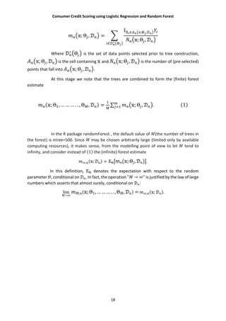
bootstrap samples from the original data set, constructs a predictor from each sample, and
decides by averaging. It is one of the most effective computationally intensive procedures to
improve on unstable estimates, especially for large, high-dimensional data sets, where finding
a good model in one step is impossible because of the complexity and scale of the problem
(Bühlmann and Yu 2002; Kleiner et al. 2014; Wager et al. 2014) However, while bagging and
the CART-splitting scheme play key roles in the random forest mechanism, both are difficult
to analyse with rigorous mathematics, thereby explaining why theoretical studies have so far
considered simplified versions of the original procedure. This is often done by simply ignoring
the bagging step and/or replacing the CART-split selection by a more elementary cut protocol.
As well as this, in Breiman’s (2001) forests, each leaf (that is, a terminal node) of individual
trees contains a small number of observations, typically between 1 and 5.
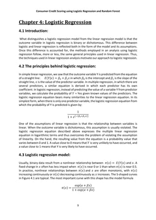
5.3 Definition of random forests:
A random forest is a classifier consisting a collection of tree-structured classifiers
{ℎ( , Θ ), = 1, … … … } where {Θ } are independent and identically distributed
random vectors and each tree casts a unit vote for the most popular class at input .
5.4 Basic principles:
Let us start with a word of caution. The term “random forests” is a bit ambiguous. For some
authors, it is but a generic expression for aggregating random decision trees, no matter how
the trees are obtained. For others, it refers to Breiman’s (2001) original algorithm. We
essentially adopt the second point of view in the present survey.
Our objective in this section is to provide a concise but mathematically precise
presentation of the algorithm for building a random forest. The general framework is
nonparametric regression estimation, in which an input random vector ∈ ⊂ ℝ is
observed, and the goal is to predict the square integrable random response ∈ ℝ by
estimating the regression
function ( ) = [ | = ]. With this aim in mind we assume that we have training sample
= ( , ), … … … . , ( , ) of independent random variables distributed as the
independent prototype pair ( , ).The goal is to use the dataset to construct an estimate
: → ℝ of the function . In this respect we say that regression function estimate is
(mean squared error) is consistent if [ ( ) − ( )] → 0 as → ∞(the expectation is
evaluated over and the sample .
A random forest is a predictor consisting of a collection of randomized
regression trees. For the tree is the family, the predicted value at the query point is
denoted by ; Θ , , where Θ , … … … . . , Θ are independent random variables
distributed same as the generic random variable Θ and independent of . In practice, the
variable Θ is used to resample the training set prior to the growing of individual trees and to
select the successive directions for splitting. In mathematical terms the tree estimate takes
the form:
18. Consumer Credit Scoring using Logistic Regression and Random Forest
18
; Θ , =
∈ ; ,
; Θ ,
∈ ∗
Where ∗
Θ is the set of data points selected prior to tree construction,
; Θ , is the cell containing and ; Θ , is the number of (pre-selected)
points that fall into ; Θ , .
At this stage we note that the trees are combined to form the (finite) forest
estimate
( ; Θ , … … … . . , Θ , ) = ∑ ; Θ , . (1)
In the R package randomForest , the default value of (the number of trees in
the forest) is ntree=500. Since may be chosen arbitrarily large (limited only by available
computing resources), it makes sense, from the modelling point of view to let tend to
infinity, and consider instead of (1) the (infinite) forest estimate
, ( ; ) = ;Θ , .
In this definition, denotes the expectation with respect to the random
parameter , conditional on . In fact, the operation " → ∞" is justified by the law of large
numbers which asserts that almost surely, conditional on :
lim
→
, ( ;Θ1,………..,Θ , ) = , ( ; ).
19. Consumer Credit Scoring using Logistic Regression and Random Forest
19
Chapter 6: An overview of LASSO:
6.1 Introduction
The “lasso” minimizes the residual sum of squares subject to the sum of absolute value of the
coefficients being less than a constant. Because of the nature of this constant it tends to
produce some coefficients that are exactly 0 and hence give interpretable models.
The two standard techniques for improving the OLS estimates, subset selection
and ridge regression, both have drawbacks. Subset selection provides interpretable models
but can be extremely variable because it is a discrete process- regressors are either retained
or dropped from the model. Small changes in the data set can result in very different models
being selected and this can reduce prediction accuracy. Ridge regression is a continuous
process that shrinks coefficients and hence is more stable: however, it does not set any
coefficients to 0 and hence does not give an easily interpretable model.
The lasso shrinks some coefficients and sets others to zero and hence tries to
retain good features of both subset selection and ridge regression.
6.2 Definition
Suppose that we have the data ( , ), = 1,2, … … … , , where = , , … … … ,
are the predictor variables and are the responses. As in the regression set-up, we assume
that either the observations are independent or that the are conditionally independent
given the . We assume that are standardized so that ∑ ⁄ = 0 and ∑ = 1.⁄
Letting = , … … , , the lasso estimate , is defined by
, = argmin ∑ y − α − ∑ subject to ∑ | | ≤ .
Here ≥ 0 is a tuning parameter. Now for all , the solution for is = . We can assume
without loss of generality that = 0 and hence omit .
We can also write the lasso problem in the equivalent Lagrangian form.
yi
− α − + | | = + | |
Here we say that lasso generates sparse models, i.e. models that involves only a subset of
variables.
20. Consumer Credit Scoring using Logistic Regression and Random Forest
20
Chapter 7: Analysis of German credit data:
Here I first perform parametric classification e.g. Logistic regression, shall see how the model fits,
infer about it then I will use non-parametric classification e.g. Random Forest.
Before getting into any sophisticated analysis, the first step is to do an EDA and data
cleaning. Since both categorical and continuous variables are included in the data set,
appropriate tables and summary statistics are provided. Proportions of applicants belonging
to each classification of a categorical variable are shown in the following table (below).
Depending on the cell proportions given in the one-way table above two or more cells are
merged for several categorical predictors. We present below the final classification for the
predictors that may potentially have any influence on Creditability.
21. Consumer Credit Scoring using Logistic Regression and Random Forest
21
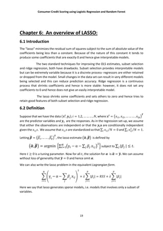
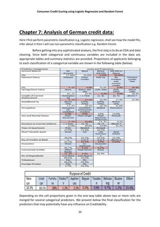
Account Balance: No account (1), None (No balance) (2), Some Balance (3)
Payment Status: Some Problems (1), Paid Up (2), No Problems (in this bank) (3)
Savings/
Stock Value: None, Below 100 DM, [100, 1000] DM, Above 1000 DM
Employment Length: Below 1 year (including unemployed), [1, 4), [4, 7), Above 7
Sex/Marital Status: Male Divorced/Single, Male Married/Widowed, Female
No of Credits at this bank: 1, More than 1
Guarantor: None, Yes
Concurrent Credits: Other Banks or Dept. Stores, None
Foreign Worker variable may be dropped from the study
Purpose of Credit: New car, Used car, Home Related, Other
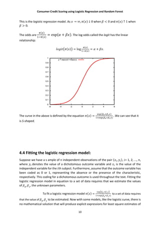
Cross-tabulation of the some of the 9 predictors as defined above with Creditability is shown
below. The proportions shown in the cells are column proportions and so are the marginal
proportions. For example, 30% of 1000 applicants have no account and another 30% have no
balance while 40% have some balance in their account. Among those who have no account
135 are found to be Creditable and 139 are found to be Non-Creditable. In the group with no
balance in their account, 40% were found to be on-Creditable whereas in the group having
some balance only 1% are found to be Non-Creditable.
| Acc.Balance
Creditability | 1 | 2 | 3 | Row Total |
--------------|-----------|-----------|-----------|-----------|
0 | 240 | 14 | 46 | 300 |
| 0.4 | 0.2 | 0.1 | |
--------------|-----------|-----------|-----------|-----------|
1 | 303 | 49 | 348 | 700 |
| 0.6 | 0.8 | 0.9 | |
--------------|-----------|-----------|-----------|-----------|
Column Total | 543 | 63 | 394 | 1000 |
| 0.5 | 0.1 | 0.4 | |
--------------|-----------|-----------|-----------|-----------|
| Payment. Status
Creditability | 1 | 2 | 3 | Row Total |
--------------|-----------|-----------|-----------|-----------|
0 | 53 | 169 | 78 | 300 |
| 0.6 | 0.3 | 0.2 | |
--------------|-----------|-----------|-----------|-----------|
1 | 36 | 361 | 303 | 700 |
| 0.4 | 0.7 | 0.8 | |
--------------|-----------|-----------|-----------|-----------|
Column Total | 89 | 530 | 381 | 1000 |
| 0.1 | 0.5 | 0.4 | |
--------------|-----------|-----------|-----------|-----------|
| Savings
Creditability | 1 | 2 | 3 | Row Total |
--------------|-----------|-----------|-----------|-----------|
0 | 217 | 34 | 49 | 300 |
| 0.4 | 0.3 | 0.2 | |
--------------|-----------|-----------|-----------|-----------|
1 | 386 | 69 | 245 | 700 |
23. Consumer Credit Scoring using Logistic Regression and Random Forest
23
In preparation of predictors to use in building a logistic regression model, we consider bivariate
association of the response (Creditability) with the categorical predictors.
Model building with 50:50 cross validation:
Only significant predictors are to be included in the logistic regression model. Since there are 1000
observations 50:50 cross-validation scheme is tried. 1000 observations are randomly partitioned
into two equal sized subsets – Training and Test data. A logistic model is fit to the Training set.
We perform backward stepwise logistic regression here. The final model after performing
stepwise regression and associated results are given below.
Call:
glm(formula = Creditability ~ Account.Balance + Duration.of.Credit..month. +
Payment.Status.of.Previous.Credit + Purpose + Credit.Amount + Value.Savings.Stocks +
Length.of.current.employment + Instalment.per.cent + Guarantors +
Duration.in.Current.address + Age..years. + Foreign.Worker, family = "binomial", data =
Train50)
Deviance Residuals:
Min 1Q Median 3Q Max
-2.8881 -0.5960 0.3079 0.6393 2.5293
24. Consumer Credit Scoring using Logistic Regression and Random Forest
24
Null deviance: 610.86 on 499 degrees of freedom
Residual deviance: 408.48 on 463 degrees of freedom
AIC: 482.48
If we want to see which variables are dropped, we can see here:
Step df Deviance Residual.df Residual.Dev AIC
1 NA NA 445 391.3381 501.3381
2 Most. Valuable. avai
lable.asset
3 0.8845622 448 392.2226 496.2226
3 Occupation 3 1.2792911 451 393.5019 491.5019
4 No.of.Credits.at.thi
s.Bank
3 2.3052671 454 395.8072 487.8072
5 No.of. dependents 1 0.3380494 455 396.1452 486.1452
6 Concurrent.Credits 2 2.7130649 457 395.8583 484.8583
7 Type.of.apartment 2 2.5642810 459 401.4226 483.4226
25. Consumer Credit Scoring using Logistic Regression and Random Forest
25
Step df Deviance Residual.df Residual.Dev AIC
8 Telephone 1 1.4482482 460 402.8078 482.8078
9 Sex...Marital.Status 3 5.6066694 463 408.4775 482.8075
Goodness of fit test:
Chi-square goodness of fit: Here test statistic = 483.2076
And − =0.9674946. A large − indicating the lack of fit.
Hosmer-Lemshow Test:
$C
Hosmer-Lemeshow C statistic
data: fit50 and TrainRspns
X-squared = 7.1672, df = 8, p-value = 0.5187
$H
Hosmer-Lemeshow H statistic
data: fit50 and TrainRspns
X-squared = 7.3264, df = 8, p-value = 0.5019
Now I do a classification table to check how accurate the model predicts with different cutoff values
of probability.
Test Data 50% Threshold 40% Threshold 75% Threshold
Creditable Non-
creditable
Creditable Non-
creditable
Creditable Non-
creditable
Creditable 350 296 54 311 39 247 103
Non-
creditable
150 80 70 94 56 50 100
Total 500 Accuracy= (70+296)/500
=73.2%
Accuracy= (311+56)/500
=73.4%
Accuracy=
(247+100)/500
=69.4%
From these I can conclude that cutoff probability 0.4 gives better accuracy in predicting than others .
Now let us have a looks how the model performs for different samples of the original data . Here I
am going to use k-fold cross validation. The most common variation of cross validation is 10-fold
cross-validation.
Generalized Linear Model
1000 samples
20 predictor
2 classes: '0', '1'
No pre-processing
26. Consumer Credit Scoring using Logistic Regression and Random Forest
26
Resampling: Cross-Validated (10 fold, repeated 10 times)
Summary of sample sizes: 900, 900, 900, 900, 900, 900, ...
Resampling results:
Accuracy Kappa
0.7478 0.3642265
Now let’s see if there is any improvement in accuracy via confusion matrix.
Confusion Matrix and Statistics
Reference
Prediction 0 1
0 74 37
1 76 313
Accuracy : 0.774
95% CI : (0.7348, 0.8099)
No Information Rate : 0.7
P-Value [Acc > NIR] : 0.0001305
Kappa : 0.4187
Mcnemar's Test P-Value : 0.0003506
Sensitivity : 0.4933
Specificity : 0.8943
Pos Pred Value : 0.6667
Neg Pred Value : 0.8046
Prevalence : 0.3000
Detection Rate : 0.1480
Detection Prevalence : 0.2220
Balanced Accuracy : 0.6938
'Positive' Class : 0
Here we can see in comparison to previous classification table we have a slight improvement
in accuracy, here we have 77.4% accuracy in predicting the true values of .
Now the question remains, is this model is a good fit? What are the effects of covariates
in misclassification? How does it affect the model? I discuss these later. First let’s see how the
nonparametric classifier e.g. Random forest performs.
Random forests are very good in that it is an ensemble learning method used for classification
and regression. It uses multiple models for better performance that just using a single tree
model. In addition, because many sample are selected in the process a measure of variable
importance can be obtain and this approach can be used for model selection and can be
particularly useful when forward/backward stepwise selection is not appropriate and when
working with an extremely high number of candidate variables that need to be reduced.
Here I do an unsupervised random forest method. Which leads to the following
results:
Call:
randomForest(formula = as.factor(Creditability) ~ ., data = Train50,
ntree = 400, importance = TRUE, proximity = TRUE)
Type of random forest: classification
Number of trees: 400
No. of variables tried at each split: 4
OOB estimate of error rate: 24%
Confusion matrix:
0 1 class.error
27. Consumer Credit Scoring using Logistic Regression and Random Forest
27
0 53 97 0.64666667
1 23 327 0.06571429
Plotting this out of bag error can help interpreting the error at the addition of each tree during
training.
The variable importance plot is a critical output of the random forest algorithm. For each
variable in your matrix it tells you how important that variable is in classifying the data. The
plot shows each variable on the y-axis, and their importance on the x-axis. They are ordered
top-to-bottom as most- to least-important. Therefore, the most important variables are at
the top and an estimate of their importance is given by the position of the dot on the x-axis.
You should use the most important variables, as determined from the variable importance
plot, in the PCA, CDA, or other analyses. Typically, we should look for a large break between
variables to decide how many important variables to choose. This is an important tool for
reducing the number of variables for other data analysis techniques, but we should be careful
not to have either too few variables (that won't separate the data) or too many variables (that
will over explain the differences). Let’s check this plot.
28. Consumer Credit Scoring using Logistic Regression and Random Forest
28
Now I will show that how random forest perform in predicting the credit scores. Measure of
accuracy will be given via confusion matrix.
Confusion Matrix and Statistics
Reference
Prediction 0 1
0 88 53
1 62 297
Accuracy : 0.771
95% CI : (0.704, 0.8022)
No Information Rate : 0.7
P-Value [Acc > NIR] : 0.05246
Kappa : 0.2772
Mcnemar's Test P-Value : 2.865e-08
Sensitivity : 0.3400
Specificity : 0.9029
Pos Pred Value : 0.6240
Neg Pred Value : 0.8248
Prevalence : 0.3000
Detection Rate : 0.1020
Detection Prevalence : 0.1700
Balanced Accuracy : 0.6924
'Positive' Class : 0
29. Consumer Credit Scoring using Logistic Regression and Random Forest
29
So form above we have found that the accuracy in prediction is 77.1%. Which is quite an
improvement from the logistic regression procedure we performed before.
Ultimately these statistical decisions must be translated into profit consideration
for the bank. Let us assume that a correct decision of the bank would result in 35% profit at
the end of 5 years. A correct decision here means that the bank predicts an application to be
good or credit-worthy and it actually turns out to be credit worthy. When the opposite is
true, i.e. bank predicts the application to be good but it turns out to be bad credit, then the
loss is 100%. If the bank predicts an application to be non-creditworthy, then loan facility is
not extended to that applicant and bank does not incur any loss (opportunity loss is not
considered here). The cost matrix, therefore, is as follows:
Predicted
Actual Creditworthy Creditworthy Non-Creditworthy
+0.35 0
Non-creditworthy -1.00 0
Out of 1000 applicants, 70% are creditworthy. A loan manager without any model would incur
[0.7*0.35 + 0.3 (-1)] = - 0.055 or 0.055 unit loss. If the average loan amount is 3200 DM
(approximately), then the total loss will be 1760000 DM and per applicant loss is 176 DM.
Actual Prediction by logistic regression Prediction by random forest
50%
threshold
40%
threshold
75%
threshold
Creditable Creditable Creditable Creditable
Creditable 0.592 0.622 0.494 0.594
Non-
creditable
0.16 0.188 0.1 0.124
Per
applicant
profit
0.0472 0.0297 0.0729 0.0839
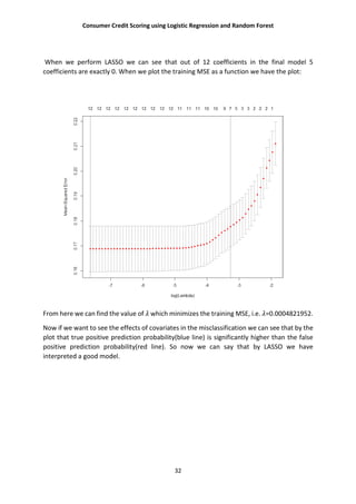
Random forest shows a good per unit profit.
30. Consumer Credit Scoring using Logistic Regression and Random Forest
30
Limitations: Though we have performed logistic regression and random forest and get an
accuracy of predicting 73.4 and 77.1 respectively (not considering the k-fold cross validation
case). But did it actually perform that well?
If we plot a scatterplot for the data, we can see lots of correlations among the variables.
In r we perform a scatterplot matrix and see too much correlations among the variables. Plot
is given below.
From the plot we can see that there is lots of correlations among the 12 covariates which we
found after performing logistic regression. So there exists multicollinearity. One way to
improve from this is to perform a variable reduction technique, e.g. Principal component
analysis. After performing principal component analysis it can be seen that, the first principal
component explains 95% of the variation which is the proof of existence of multicollinearity.
Now as we have 12 covariates in the improved model but it is really difficult to check the
effects of all these covariates in the misclassification. So we look into the absolute value of
t-statistic of each model parameter to assess the relative importance of each individual
predictor of the model. Now selecting only three most important predictors and vary them
according to their levels and fix remaining nine predictors to their mean effect. Then we try
to plot the true positive prediction probability i.e. ( = ) and false positive prediction
probability i.e ( ≠ ) against the samples. The result comes out as:
31. Consumer Credit Scoring using Logistic Regression and Random Forest
31
As we can see from the above plot the blue line represent true positive prediction
probability and the red line represent false positive prediction probability. As both the red
line cuts the blue line in many points which should be higher than the red line, we can
conclude that the misclassification error is highly affected by the covariate.
Now as the first PC explains most of the variation, I use the first pc to model the data
then plot the graph in the above mentioned way to see is there any improvement.
We can see from the graph that there is slight improvement as the blue line is a bit higher
though still there is a cut between red and blue line.
Then what should be the procedure to improve this fact? The answer is LASSO.
32. Consumer Credit Scoring using Logistic Regression and Random Forest
32
When we perform LASSO we can see that out of 12 coefficients in the final model 5
coefficients are exactly 0. When we plot the training MSE as a function we have the plot:
From here we can find the value of which minimizes the training MSE, i.e. =0.0004821952.
Now if we want to see the effects of covariates in the misclassification we can see that by the
plot that true positive prediction probability(blue line) is significantly higher than the false
positive prediction probability(red line). So now we can say that by LASSO we have
interpreted a good model.
33. Consumer Credit Scoring using Logistic Regression and Random Forest
33
Conclusion: As the conclusion of this data analysis we note these following points:
Non-parametric classification methods are working well than the parametric
classification methods. As it produces better accuracy
Though it seems that gaining 77% accuracy is really very good but from a covariate
specific view we can see that there is high misclassification error. Which in turn proves
that the model fitting is not good. Some other actions should be required.
As the data set contains so many predictors and large number of observations and as
the covariates are highly correlated it is obvious that there is something wrong with
the model.
The above two points indicate a separate method to be implemented, which can be
LASSO as it makes most of the coefficients zero indicating a better model prediction
and it also reduces the effect of covariates in misclassification as seen in the last graph.
34. Consumer Credit Scoring using Logistic Regression and Random Forest
34
Appendix:
Appendix 1:
R codes:
# loading the data set
DATA<-read.csv("C:/Users/Hirak/Desktop/german_credit.csv",header=TRUE)
View(DATA)
names(DATA)
attach(DATA)
#Performing EDA
margin.table(prop.table(table(Duration.in.Current.address,Most.valuable.available.asset,Concurrent
.Credits,No.of.Credits.at.this.Bank,Occupation,No.of.dependents,Telephone,Foreign.Worker)),1)
margin.table(prop.table(table(Duration.in.Current.address,Most.valuable.available.asset,
Concurrent.Credits,No.of.Credits.at.this.Bank,Occupation,No.of.dependents,Telephone,
Foreign.Worker)),2)
margin.table(prop.table(table(Duration.in.Current.address,Most.valuable.available.asset,
Concurrent.Credits,No.of.Credits.at.this.Bank,Occupation,No.of.dependents,Telephone,
Foreign.Worker)),3)
margin.table(prop.table(table(Duration.in.Current.address,Most.valuable.available.asset,
Concurrent.Credits,No.of.Credits.at.this.Bank,Occupation,No.of.dependents,Telephone,
Foreign.Worker)),4)
margin.table(prop.table(table(Duration.in.Current.address,Most.valuable.available.asset,
Concurrent.Credits,No.of.Credits.at.this.Bank,Occupation,No.of.dependents,Telephone,
Foreign.Worker)),5)
margin.table(prop.table(table(Duration.in.Current.address,Most.valuable.available.asset,
Concurrent.Credits,No.of.Credits.at.this.Bank,Occupation,No.of.dependents,Telephone,
Foreign.Worker)),6)
margin.table(prop.table(table(Duration.in.Current.address,Most.valuable.available.asset,
Concurrent.Credits,No.of.Credits.at.this.Bank,Occupation,No.of.dependents,Telephone,
Foreign.Worker)),7)
margin.table(prop.table(table(Duration.in.Current.address,Most.valuable.available.asset,
Concurrent.Credits,No.of.Credits.at.this.Bank,Occupation,No.of.dependents,Telephone,
Foreign.Worker)),8)
#cross tables
library(gmodels)
CrossTable(Creditability,Acc.Balance,digits=1,prop.r=F,prop.t=F, prop.chisq=F, chisq=F)
35. Consumer Credit Scoring using Logistic Regression and Random Forest
35
CrossTable(Creditability,Payment.status, digits=1,prop.r=F, prop.t=F, prop.chisq=F, chisq=F)
CrossTable(Creditability,Savings,digits=1,prop.r=F,prop.t=F, prop.chisq=F, chisq=F)
CrossTable(Creditability,Employment.length,digits=1,prop.r=F, prop.t=F, prop.chisq=F, chisq=F)
CrossTable(Creditability,Sex_marital_status,digits=1,prop.r=F, prop.t=F, prop.chisq=F, chisq=F)
CrossTable(Creditability,No_of_Credits,digits=1,prop.r=F, prop.t=F, prop.chisq=F, chisq=F)
CrossTable(Creditability,Guarantor,digits=1,prop.r=F, prop.t=F, prop.chisq=F, chisq=F)
CrossTable(Creditability,Concurrent_credit,digits=1,prop.r=F, prop.t=F, prop.chisq=F, chisq=F)
CrossTable(Creditability,Purpose_of_credit,digits=1,prop.r=F,prop.t=F, prop.chisq=F, chisq=F)
CrossTable(Creditability,Type.of.apartment,digits=1,prop.r=F,prop.t=F, prop.chisq=F, chisq=F)
CrossTable(Creditability,No.of.dependents,digits=1,prop.r=F,prop.t=F, prop.chisq=F, chisq=F)
CrossTable(Creditability,Instalment.per.cent,digits=1,prop.r=F,prop.t=F, prop.chisq=F, chisq=F)
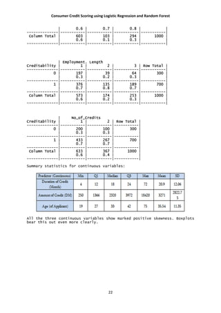
#Summary statistics for continuous variables
summary(Duration.of.Credit..month.);sd(Duration.of.Credit..month.)
summary(Credit.Amount);sd(Credit.Amount)
summary(Age..years.);sd(Age..years.)
#boxplot for cont. variables
par(mfrow=c(2,2))
boxplot(Duration.of.Credit..month., bty="n",xlab = "Credit Month", cex=0.4) # For boxplot
boxplot(Credit.Amount, bty="n",xlab = "Amount", cex=0.4)
boxplot(Age..years., bty="n",xlab = "Age", cex=0.4)
# Logistic model
for (i in c(2,4:5,7:13,15:20)){
DATA[,i] <- as.factor(DATA[,i])
}
nrow(DATA)
set.seed(50) # setting the random number seed for splitting the dataset
indexes = sample(1:nrow(DATA), size=0.5*nrow(DATA)) # Random sample of 50% of row numbers
created
Train50 <- DATA[indexes,]
Test50 <- DATA[-indexes,]
indVariables <- colnames(DATA[,2:21]);indVariables
36. Consumer Credit Scoring using Logistic Regression and Random Forest
36
# getting the independent variables, the last column is the dependent variable
rhsOfModel <- paste(indVariables,collapse="+")
# creating the right hand side of the model expression
rhsOfModel
model <- paste("Creditability ~ ",rhsOfModel)
# creating the text model
model
frml <- as.formula(model) # converting the above text into a formula
frml
library(MASS) # loading the library MASS for stepwise regression
TrainModel <- glm(formula=frml,family="binomial",data=Train50)
# building the model on training data with LOGIT link (family = binomial
finalModel <- step(object=TrainModel)
summary(finalModel)# stepwise regression
finalModel$coefficients[1:21]
sum(residuals(finalModel,type="pearson")^2)
deviance(finalModel)
1-pchisq(deviance(finalModel),df.residual(finalModel))
summary(object=finalModel)
finalModel$anova
finalModel$fitted.values
fit50 <- fitted.values(finalModel)
fit50
library(MKmisc) # loading the library MKmisc for Hosmer Lemeshow Goodness of fit
HLgof.test(fit=fit50,obs=TrainRspns)
library(pROC) # loading library pROC for ROC curve
TestPred <- predict(object=finalModel,newdata=Test50, type="response")
# predicting the testing data
TestPredRspns <- ifelse(test= TestPred < 0.75, yes= 0, no= 1)
#Random Forest
library(randomForest)
38. Consumer Credit Scoring using Logistic Regression and Random Forest
38
lines(f2_1,col="red",lwd=2)
lines(f1_1,col="blue",lwd=2)
#lasso
x <- as.matrix(Train50_DT[, 2:13])
y <- as.matrix(Train50_DT[, 1])
cv <- cv.glmnet(x, y,nfolds = 100)
plot(cv)
mdl <- glmnet(x, y,lambda = cv$lambda.1se)
mdl$beta
plot.glmnet(mdl)
bestlam=cv$lambda.min
plot(f1_1,ylim=c(0.0,1),lwd=2)
lines(f1_1,col="blue",lwd=2)
lines(f2_1,col="red",lwd=2)
Appendix:2
Data set link: http://www.statistik.lmu.de/service/datenarchiv/kredit/kredit_e.html
For the description of variables and more information please go to this link .
39. Consumer Credit Scoring using Logistic Regression and Random Forest
39
ACKNOWLEDGEMET
It is an opportunity with much pleasure to acknowledge all those person, from whom I
received considerable help through the course of my dissertation work.
First and foremost, I would like to offer my profound deepest gratitude and
record my sense of obligation to Dr. Sibnarayan Guria, Head of the department,
Department of Statistics. His cordiality, civility and amicableness provided an apt
platform for me to work. His superintendence, suggestion and discussion at every stage
have helped me immensely to carry out this work in a better way.
I am sure, there are no such thanking words to express my gratitude to Dr.
Sumanta Adhya, Assistant Professor, Department of Statistics, West Bengal State
University without whose heartiest cooperation, guidance, suggestion my dissertation
work, may not be successfully completed. I have been highly profited by lively discussions
on various aspects of Knowledge, Computation and Programming during my dissertation
work.
I am grateful and thankful to all my classmates for their cooperation and
continuous support in various aspects of the work.
Last but not the least; I am grateful to all those people, who have helped me
directly or indirectly in case of successful completion of dissertation work.
40. Consumer Credit Scoring using Logistic Regression and Random Forest
40
References
Anderson, R. (2007). The Credit Scoring Toolkit: Theory and Practice for Retail
Credit Risk Management and Decision Automation
Carling, K; Jacobson, T; Linde, J and Roszbach, K. (2002). Capital Charges under
Basel II: Corporate Credit Risk Modeling and the Macro Economy Sveriges
Riksbank Working Paper Series No. 142
Hosmer, D.W. and Lemeshow, S. (2000). Applied Logistic Regression Second
Edition
Breiman L ( 2001) Random forests. Mach Learn 45:5–32
Breiman L ( 2003a) Setting up, using, and understanding random forests V3.1.
https://www.stat.berkeley.edu/~breiman/Using_random_forests_V3.1.pdf
Robert.J.Tibshirani(1996). Regression Shrinkage and selection via the LASSO,JASA
B(1996),58,No.1,pp.267-288