Group 3 III-CCSAD

1. PRODUCTION
By Group 3 III-CCSAD

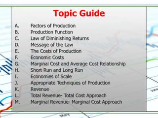
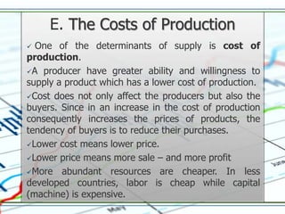
2. Topic Guide
A. Factors of Production
B. Production Function
C. Law of Diminishing Returns
D. Message of the Law
E. The Costs of Production
F. Economic Costs
G. Marginal Cost and Average Cost Relationship
H. Short Run and Long Run
I. Economies of Scale
J. Appropriate Techniques of Production
K. Revenue
L. Total Revenue- Total Cost Approach
M. Marginal Revenue- Marginal Cost Approach

3. Man can produce goods and services
without utilizing land, labor, capital or
management .
Goods produced by man are called
economic goods . However there are goods
which are produce by nature. Such goods are
called free goods.
In the production of goods and services,
the various factors of production receive their
corresponding payment like wages rents,
interest and normal profits.

4. A. Factors of Production
Land- is an original gift of nature. It includes the soil,
river, oceans, mountains etc…
Labor- is an exertion of physical and mental efforts
of individuals. This implies not only to workers, farmers
or laborers but also to professionals like accountants
economist and scientist.
Capital- is a finished product which is used to
produce goods. However, money is a medium of
exchange. It can not produce goods it can only buy
goods.
Entrepreneur- is an organizer and coordinator of the
land, labor and capital.

5. B. Production Function
Production- is the creation of goods and services to
satisfy human wants.
The factors of production are called the inputs of
production, and the goods and services that have been
created by the inputs are called outputs of
production.
The factors of production are classified as fixed
factor (fixed input) and variable factor (variable
input)
A fixed factor remains constant regardless of the
volume of production. This means whether you
produce or not, the factor of production is unchanged.

6. B. Production Function
In case of a variable factor, it changes in accordance
with the volume production. No production means no
variable factor. More production means more variable
factors.
The process of transforming both fixed and variable
inputs into finished goods and services is called theory
of production. The quantity and quality of goods and
services being produced depend on the state of
technology.

7. C. Law of Diminishing Returns
Also known as the law of diminishing marginal
productivity. It is a basic law of economics and
technology.
The law states that when successive units of variable
input (like farmers) work with a fixed input (like one
hectare of land), beyond a certain point the additional
product ( output) produced by each additional unit of
variable, input decreases.
The validity of the law of diminishing returns is based
on two assumptions. The successive units of a variable
input to should be identical, and the same technology
is applied.

8. C. Law of Diminishing Returns
It is noted that in the work combination of variable
input and fixed input, total output and additional
output (or marginal product) increase up to a certain
point.
Beyond this point, the rate of increase of total product
declines, and later on total product decreases as more
units of a variable factor are employed.
In the case of marginal product, it also diminishes
beyond a certain point until it reaches negative returns
as more variable inputs are added (see table and
graph).

9. Table 4.1. The Law of Diminishing Returns
3-Hectare Rice Field
Farmers Total Product Marginal Product
1 40 0
2 55 15
3 75 20
4 100 25
5 120 20
6 135 15
7 145 10
8 145 0
9 135 -10
10 120 -15

10. Figure 4.1. The Law of Diminishing Returns

11. As shown in Table 4.1, the contribution of farmer 1 to
production is 40 cavans. Marginal product is 0 because
there is no additional farmer yet. The contribution of
farmer 3 to production is 15 cavans. This is the
additional or marginal product produced by farmer 2.
Total product of the 2 farmers (farmer 1 and farmer 2)
is 55 cavans (40 + 15). Up to farmer 4, marginal
product is increasing. But after this point, marginal
product decreases progressively until it becomes
negative.

12. D. Message of the Law
The production of goods greatly depends on available
resources or inputs.
Marginal product is defined as the additional product
brought about by one additional unit of a variable input
(farmer).
It is noted that when marginal product increases,
total product also increases. When marginal product
decreases, total product increases and at a decreasing
rate, and when marginal product is below zero or
negative, total product falls.
The message of the law is that there is a proper
combination of variable input and a fixed input in
order to attain the maximum output.

13. E. The Costs of Production
 One of the determinants of supply is cost of
production.
A producer have greater ability and willingness to
supply a product which has a lower cost of production.
Cost does not only affect the producers but also the
buyers. Since in an increase in the cost of production
consequently increases the prices of products, the
tendency of buyers is to reduce their purchases.
Lower cost means lower price.
Lower price means more sale – and more profit
More abundant resources are cheaper. In less
developed countries, labor is cheap while capital
(machine) is expensive.

14. F. Economic Costs
Total Cost- is the sum total cost of production.
Normal profit is a part of total cost of production.
Pure profit is the excess of the cost production.
Total cost is also equivalent to fixed cost plus variable
cost
Fixed Cost- remains constant regardless of the
volume of production. If there is no production, there is
still cost.
Variable Cost- changes in proportion to volume of
production. If there is no production, there is no cost.
More production means more cost.

15. F. Economic Costs
Average Cost- also called unit cost. It is equivalent
to total cost divided by quantity.
AC = TC
Q
Marginal Cost – additional or extra cost brought
about by producing one additional unit.
MC = TC
Q
Explicit Cost- expenditure cost.
Implicit Cost- non-expenditure cost. They do not
pay. You do not pay rent to your own land.
Opportunity Cost- opportunity or alternative benefit.

16. Figure 4.2. Total, fixed, and variable costs.
6
5
4
3 Series 2
Series 1
2
1
0
Category 1 Category 2 Category 3 Category 4

17. G. Marginal Cost and Average Cost
When MC is falling, it pulls down AC, and when MC is
rising, it pulls up AC.
At the start of production, AC is greater than MC.
But when MC continues to rise, it reaches a point where
it is equal to Figure 4.3, the MC curve intersects the AC
curve at its lowest point. Beyond this intersection
point, the curve rises at a faster rate than the AC curve.
The AC curve has a U-Shape. This explains the fact that
AC is high when less units are produced.
The effects of MC on AC are due to mathematical
relationship. As long as MC is less than AC, the latter falls.
AC will only rise if MC is more than AC as shown in Table
4.2. illustrated in

18. Figure 4-3. MC and AC Relationship – when MC is
falling, it pulls down AC; when MC is rising, it pulls up AC.
MC intersects AC at its lowest portion.

19. Table 4.2: Mathematical relationship between MC and AC.
Product Cost Total AC MC
Cost
1 P 160 P 160 P 160 P 140
2 140 300 150 120
3 120 420 140 140
4 140 560 140 160
5 160 720 144 180
6 180 900 150
200 1,100 200
157.14

20. Said table, the cost of product 1 is P160. Total cost is
P160 and AC is P160 (P160 divided by 1). The cost of an
additional product (product 2) is P140. Total cost of
product 1 and 2 is P300. AC is P150 (300 divided by 2).
MC is P140 which is the cost of the additional product.
The cost of the third product is P120. The total cost of the
3 products is P420. AC is P140 while MC is P120. However,
the cost of the fourth product is P140 which is higher than
the cost of product 3. Total cost is P560, AC is P140 and
MC is also P140. At this point MC equals AC.
It is noted that as MC increases, AC also rises, as shown
in table. MC is equal at the point when AC is at the lowest
point.

21. H. Short Run and Long Run
Short run refers to a period of time which is too short
to allow an enterprise to change its plant capacity, yet
long enough to allow a change in its variable resources.
Cost of production under the short-run period is both
fixed and variable.
Long run refers to a period of time which is long
enough to permit a firm or enterprise to alter all its
resources or inputs(both fixed and variable factors).

22. I. Economies of Scale
Can be classified as:
 External Economies of Scale
- Factors outside the firm or enterprise
- Contribute to the efficiency of the latter in terms
of increased output and decreased unit cost of
production
 Internal Economies of Scale
- Factors inside the firm or enterprise
- Contribute to the efficiency of the latter

23. Note:
• Firms that enjoy both scales have become
very efficient and big
• They survived competition and therefore
have remained in the industry
• They are capable of undertaking mass
production which incurs a lower average cost
of production
• They are involved on global supply of goods;
and they have maximized their profits

24. I. Appropriate Techniques of Production
 Based on the law of supply and demand, resources
which are abundant have lower prices than those which
are scarce.
 There is surplus of labor in less developed
countries, on the other hand highly developed countries
which their price of labor is high because it is not
abundant.
• Labor-Intensive Technology
Pros
More labor inputs and less capital inputs
More plentiful resources should be utilized
because these are cheaper.

25. I. Appropriate Techniques of Production
• Why should they use this
•Capital inputs are imported, and usually expensive. Poor
countries can hardly afford to purchase them with their small
foreign exchange earnings.
 Success of China
•A huge human resource had been properly utilized, almost
100 percent of labor input.
•They manufactured their own tools of production; never
bought western technology.
•It resulted that their rural development program has been
one of the most successful program in the world.
•It didn’t need foreign assistance, so it should be a lesson to
poor countries who actually depend on western economic
development

26. I. Appropriate Techniques of Production
• Capital-Intensive Technology
- Technology used by Western countries, mainly
Americans and Europeans.
- Capital is cheaper in Western countries while labor is
expensive, in contrary to the Eastern countries.
Pros
• Uses more capital inputs and less labor input.
• In many economic activities, their operations are
computerized
• Such modern technology does not adversely affect the
labor force, because there has been an increasing
demand for workers in other sectors. Thus making this
kind of technology almost flawless and perfect.

27. J. Revenue
Cost of production refers to the total payments by
a firm to the owners of the factors of production
like land, labor, capital and entrepreneur.
These are other expenditure –side of a firm in the
process of creating goods and services. For a firm
to remain in business, it has to earn an income
which is greater than its expenses .
 The income side of a firm is called revenue. The
difference between cost and revenue is either profit
or loss, depending on which one is higher.

28. K. Total Revenue – Total Cost Approach
•Total Revenue = price times units sold
•TR = P *Q
•Total Revenue – Total Cost = Profit
Rule: if total revenue is greater than variable
cost, operates; if total revenue is less than
variable cost, shut down.
7,000 – total revenue
10,000 – fixed cost of the firm
5,000 – variable cost
---------
15,000 – Total cost

29. K. Total Revenue – Total Cost Approach
The Rules Are:
TR > TC: Produce more
TR < TC: Stop production
TR = TC: Maintain production
•Profit Maximization(under pure competition)

30. M. Marginal Revenue – Marginal Cost Approach
Marginal revenue is the additional income of a firm
brought about by producing and selling one additional
unit of a product.
The rule is: if marginal revenue is greater than marginal
cost, increase production; if marginal revenue is less than
marginal cost do not increase production.
Profit maximization of a firm is attained when MR=AC.
It can be stated therefore: profit maximization is attained
at a point where price equals marginal cost (P = MC).