Cardinal utility theory states that utility or satisfaction derived from consuming goods can be measured numerically. Total utility is the aggregate satisfaction from consuming all units of a good, while marginal utility is the satisfaction from an additional unit. The law of diminishing marginal utility posits that additional units of a good provide less additional satisfaction. Ordinal utility theory argues that utility cannot be measured, but preferences can be ranked or compared. Indifference curves depict combinations of goods that provide equal satisfaction. Budget constraints show combinations of goods that can be purchased given an income level. Consumer equilibrium occurs when a consumer maximizes satisfaction given prices and income. 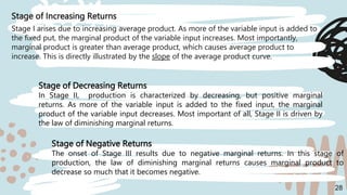Production involves inputs like labor, capital and land. The production function shows the relationship between inputs

1. THE THEORY OF
CONSUMER
BEHAVIOR
THE THEORY OF
CONSUMER
BEHAVIOR

2. 2
2
Utility refers to the degree of
satisfaction per unit of
consumption.

3. Cardinal Utility Theory
developed over the years with significant contributions from
different economists, notably Economist Alfred Marshall.
3
Cardinal Utility Theory
KEY CONCEPTS
Cardinal means that something can be
measured in numerical terms
Theory is a set of assumptions or collection of
generalization. “QUANTIFIABLE”
Utility refers to the level of satisfaction
which could change according to the
situation

4. 4
Utils refers to the unit of measurement for
satisfaction
Total Utility is the aggregate utility derived by a consumer after
consuming all the available units of a commodity. Thus, it is the
sum of all the utilities accruing from each individual units of the
commodity
Marginal Utility is the utility flowing from an additional unit
of a commodity, over and above what had been consumed
Saturation Point refers to the peak point of
the total utility curve

5. 5
Total Utility and Marginal
Utility Schedule

6. 6
Total Utility
& Marginal
Utility Curve

7. 7
LETS PRACTICE!!!

8. Law of Diminishing
Marginal Theory
states that as one consumes more and more
of a particular good, additional or extra
satisfaction decreases.
Law of Diminishing
Marginal Theory

9. Ordinal Utility Theory
also called Indifference theory, states that
utility is not measurable but can only be
ranked or compared.
in this theory, we assumed that people know
what they like, their choice is consistent, and
that they prefer more to less, But we also
recognize that people having different
perspectives.
9
Ordinal Utility Theory

10. 10

11. Indifference Curve
shows different combinations of two goods
that can be consumed that yield the same
level of satisfaction or utility.
11
Indifference
Curve

12. 12
Peter has 1 unit of food and 12 units of clothing. Now, we
ask Peter how many units of clothing is he willing to give up
in exchange for an additional unit of food so that his level of
satisfaction remains unchanged.
Peter agrees to give up 6 units of clothing for an additional
unit of food. Hence, we have two combinations of food and
clothing giving equal satisfaction to Peter as follows:
1. 1 unit of food and 12 units of clothing
2. 2 units of food and 6 units of clothing
Combination
• A
• B
• C
• D
Food
• 1
• 2
• 3
• 4
Clothing
• 12
• 6
• 4
• 3

13. 13
Indifference Map is a series of
indifferent curve

14. Budget Constraint
14
Budget Constraint
Budget Line
It is a locus of points that shows different
combinations of two goods that can be purchased given
the same money income or budget
It depicts the consumer choices between two
products.
Budget Function
A mathematical equation showing various
combinations of two goods that can be purchased given
the same budget or income.
Budget= PxQx+ PyQy

15. 15
Example:
Given Px= 10, Py=20 and Budget (B)=200. The combination
of good X and Y that can be purchased is determined by:
Budget= PxQx+PYQy
200 = 10 Qx + 20 Qy

16. 16
Budget Schedule
A list or table that shows various
combinations of two goods that can be purchased
given the same money income.
Budget= PxQx+ PyQy
Qx Qy
A 0 10
B 4 8
C 10 5
D 16 2
E 20 0

17. 17
Qx Qy
A 0 10
B 4 8
C 10 5
D 16 2
E 20 0
0
2
4
6
8
10
12
0 5 10 15 20 25
E
D
C
Budget Line
B
A

18. Consumer Equilibrium
The state of balance achieved by an end user of
products that refers to the amount of goods and
services they can purchase given their present level
of income and the current level of prices. Consumer
equilibrium allows a consumer to obtain the most
satisfaction possible from their income.
18
Consumer Equilibrium

19. Theory of production &
Cost
Theory of production &
cost

20. Production Function
OUTPUT=f( inputs)
The OUTPUT is dependent on or is a function of the
factors of production or INPUTS used by the firm.
Inputs can be found and classified into LAND,
LABOR, CAPITAL, and ENTREPRENEUR. The
production function has a DIRECT RELATION
between input and output.
20
Production
Function

22. Production Periods
22
Long-run period is a production period in
which all the inputs used in production of
the firm are variable inputs.
Very short-run period or the immediate
period is a production period in which all
factors of production used by the firm are
fixed inputs.
Short-run period is a production period
in which some inputs used by the firm
are fixed while others are variable.

23. Law of Diminishing
Marginal Returns
Law of Diminishing
Marginal Returns
The law states that as successive units of
variable inputs are added to fixed inputs,
total product increases at an increasing
rate, continuously increases at a
decreasing rate and at a certain point total
product declines.

24. 24
Total Product, Marginal Product and Average
Product

25. Average Product (AP) is the total product
per unit of the variable input.
Formula: AP = TP / Labor
25
Marginal Product (MP) is the additional or extra product
contributed by the last worker.
Formula: MP = ∆TP / ∆L

26. 26
Law of Diminishing Marginal Returns and
the Stages of Production

27. 27
The three stages of production are characterized by the
slopes, shapes, and interrelationship of the total, marginal,
and average product curves.
Three Stages of Production
Three Stages of
Production

28. Stage of Increasing Returns
Stage I arises due to increasing average product. As more of the variable input is added to
the fixed put, the marginal product of the variable input increases. Most importantly,
marginal product is greater than average product, which causes average product to
increase. This is directly illustrated by the slope of the average product curve.
28
Stage of Negative Returns
The onset of Stage III results due to negative marginal returns. In this stage of
production, the law of diminishing marginal returns causes marginal product to
decrease so much that it becomes negative.
Stage of Decreasing Returns
In Stage II, production is characterized by decreasing, but positive marginal
returns. As more of the variable input is added to the fixed input, the marginal
product of the variable input decreases. Most important of all, Stage II is driven by
the law of diminishing marginal returns.

29. Economic Cost
payment for the inputs that the firm uses in the
production processes.
29
Economic Cost
It does not only include those payments to
outside to supply the inputs called explicit cost,
but also the implicit cost
The firm in order to produce the goods
and services needs inputs like land,
labor, capital, and entrepreneur which
may be owned by firm itself or by
consumers or household.

30. are monetary
expenditures
paid to
outsiders who
supply the
inputs.
are the cost of self
owned or self employed
resources. The valuation
of the supposedly
payment or income of
the firm is important to
be included because of
the opportunity cost
concept.
Implicit
Costs
measures things that
must be given up or
sacrificed when one
chooses one alternative
over the other.
Example:
if you decide to
quit from your job and
run a business the salary
you give up is the
opportunity cost.
30
Economic
Costs
Opportunity
Cost

31. Mathematical Definition of Cost Function
The table shows that if the firm operates in the immediate period, all cost are fixed cost.
PRODUCTION
PERIOD
TOTAL COST AVERAGE COST MARGINAL COST
Immediate period TC=TFC AFC = TFC/Q
ATC = TC/Q
AFC = TFC/Q
AVC = TVC/Q
ATC =
AFC+AVC
Short-run
period
TC =
TFC+TVC
MC=
∆𝑇𝐶
∆𝑄
Long -run
period
TC = TVC
ATC = TC/Q
AVC = TVC/Q
AVC = ATC
MC=
∆𝑇𝐶
∆𝑄

32. 32
In the short-run, Total Cost (TC) for the firm includes Total
Fixed Cost (TFC) and Total Variable Cost (TVC). If the firm operate
in the long run period, TC = TVC, meaning all cost are variable

33. Variable Cost, and Total Cost
for the Firm
Total Fixed Cost, Total
Variable Cost, and Total
Cost for the Firm
33
Total Fixed Costs are costs that do not vary with
output like rentals and their amount would be the
same even if output is one unit or one million units.
Total Variable Costs are costs that vary directly
with output. It is rising as more is produced and
falling as less is produced.
Total Cost is the sum of the total fixed cost and total
variable cost.
TC= TFC+TVC

34. 34
Output Total
Fixed
Cost
Total
Variable
Cost
Total
Cost
Average
Fixed
Cost
Average
Variable
Cost
Average
Total
Cost
Marginal
Cost
0 10 0 10 - - - -
1 19 5 15 10 5 15 5
2 10 9 19 5 4.5 9.5 4
3 10 12 22 3.33 4 7.33 3
4 10 15 25 2.5 3.75 6.25 3
5 10 19 29 2 3.8 5.8 4
6 10 25 35 1.67 4.16 5.83 6
7 10 33 43 1.43 4.71 6.14 8
8 10 43 53 1.25 5.38 6.63 10

35. 35
The Different
Cost Curves for
Hypothetical
Firm in the
Short-run

36. Production Costs in the Long-
Run
36
Production Costs in the Long-
Run

37. 37
Economies of scale exists when long-
run average costs decline as output
rises, and larger firms will be more
efficient than smaller firms.
Diseconomies of scale are said to exist in
the range where average costs rise with
increases in output.