Downloaded 115 times
![Total and Per Unit Costs
Total Variable Cost (TVC)
Total Fixed Cost (TFC)
Total Cost (TC)
Average Variable Cost (AVC)
Average Fixed Cost (AFC)
Average Total Cost (ATC)
Marginal Cost (MC)
Fixed and Variable Costs
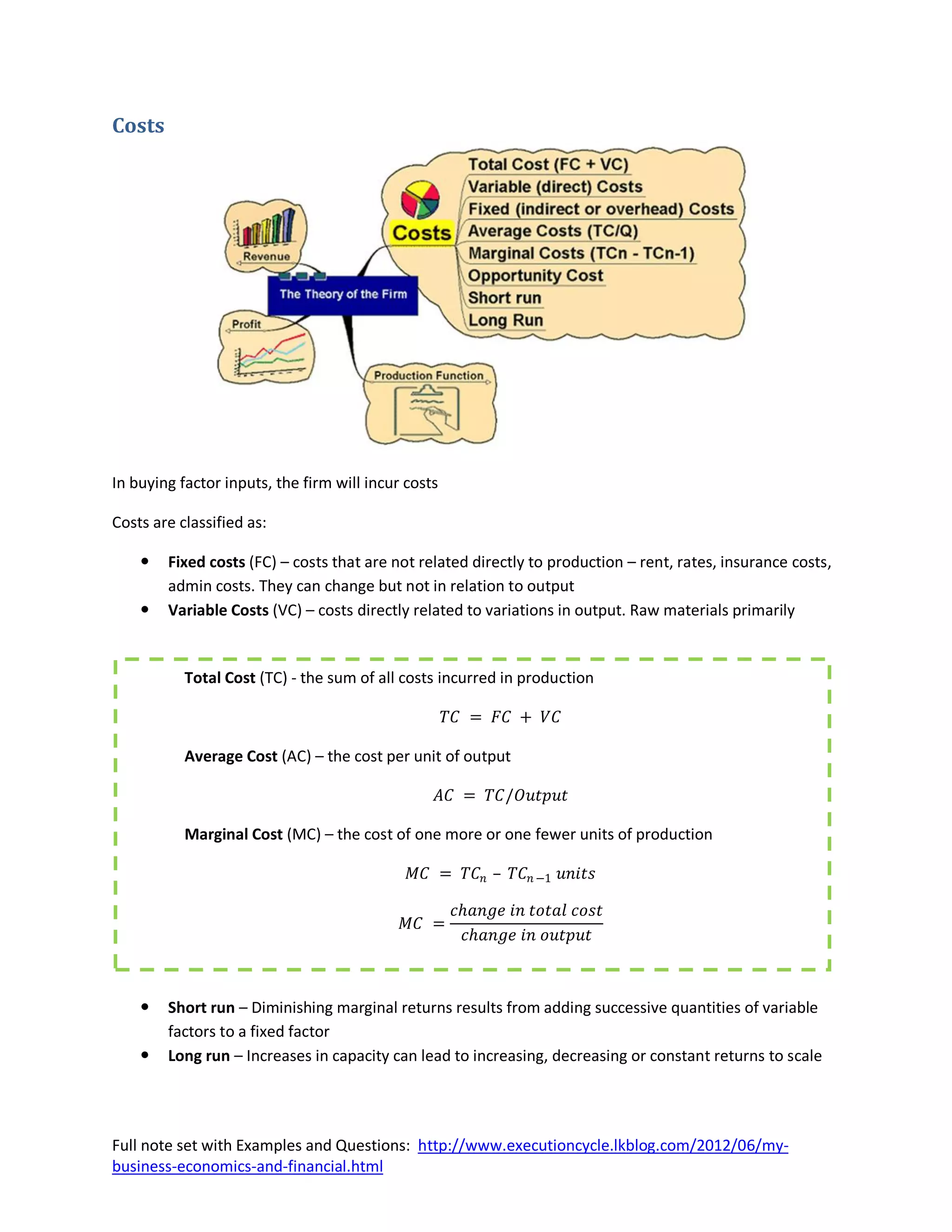
Fixed costs are those costs that do not vary with the quantity of output produced. Variable costs are
those costs that do change as the firm alters the quantity of output produced.
Average Costs
Average costs can be determined by dividing the firm’s costs by the quantity of output produced. The
average cost is the cost of each typical unit of product.
Marginal Cost
Marginal cost (MC) measures the amount total cost rises when the firm increases production by one
unit.
Question: Fill in the missing values
Three Important Properties of Cost Curves
1. Marginal cost eventually rises with the quantity of output. [Law of Diminishing Marginal
Returns]
2. The average-total-cost curve is U-shaped.
3. The marginal-cost curve crosses the average-total-cost curve at the minimum of average total
cost.
Full note set with Examples and Questions: http://www.executioncycle.lkblog.com/2012/06/my-
business-economics-and-financial.html](https://image.slidesharecdn.com/4-thetheoryofthefirmandthecostofproduction-120610115228-phpapp02/75/4-the-theory-of-the-firm-and-the-cost-of-production-9-2048.jpg)
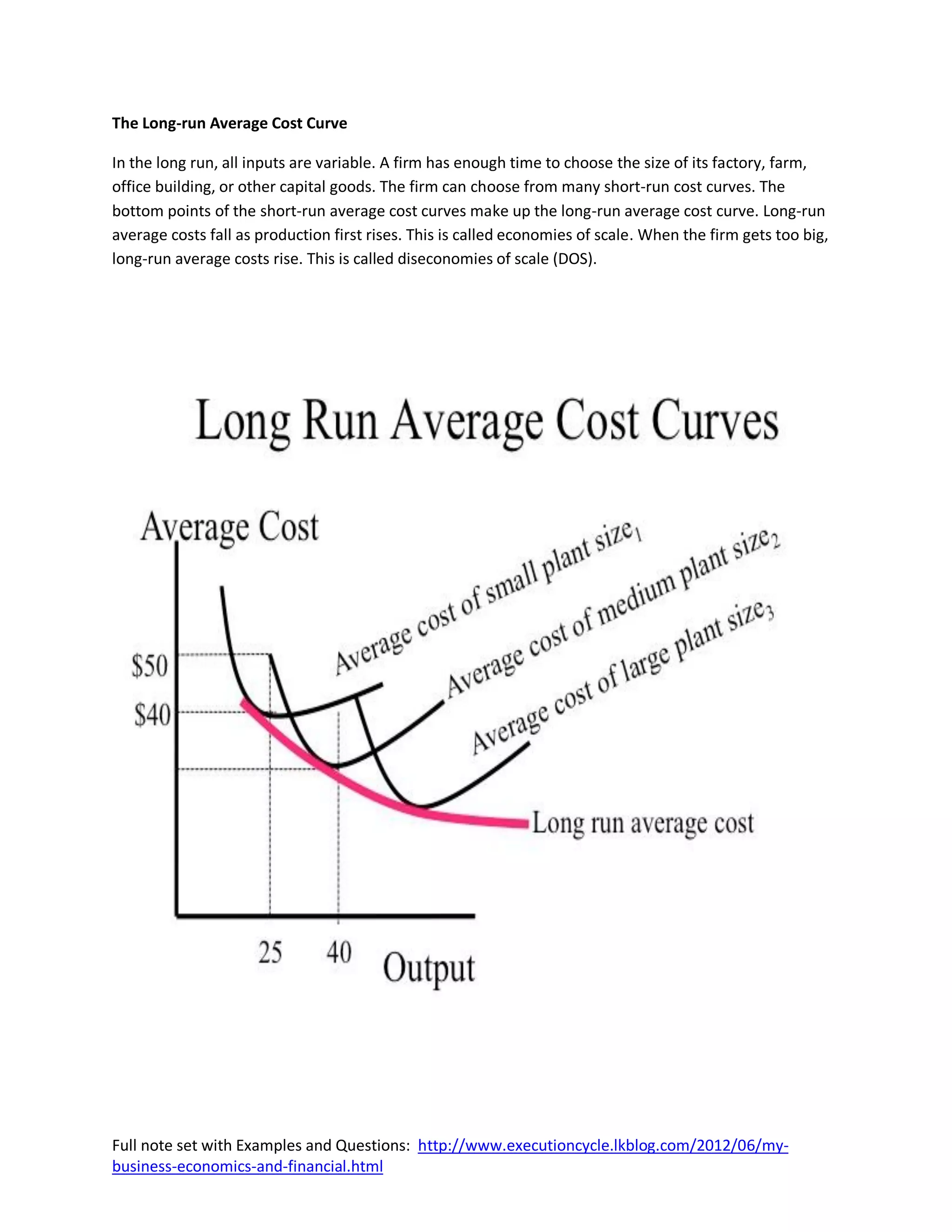

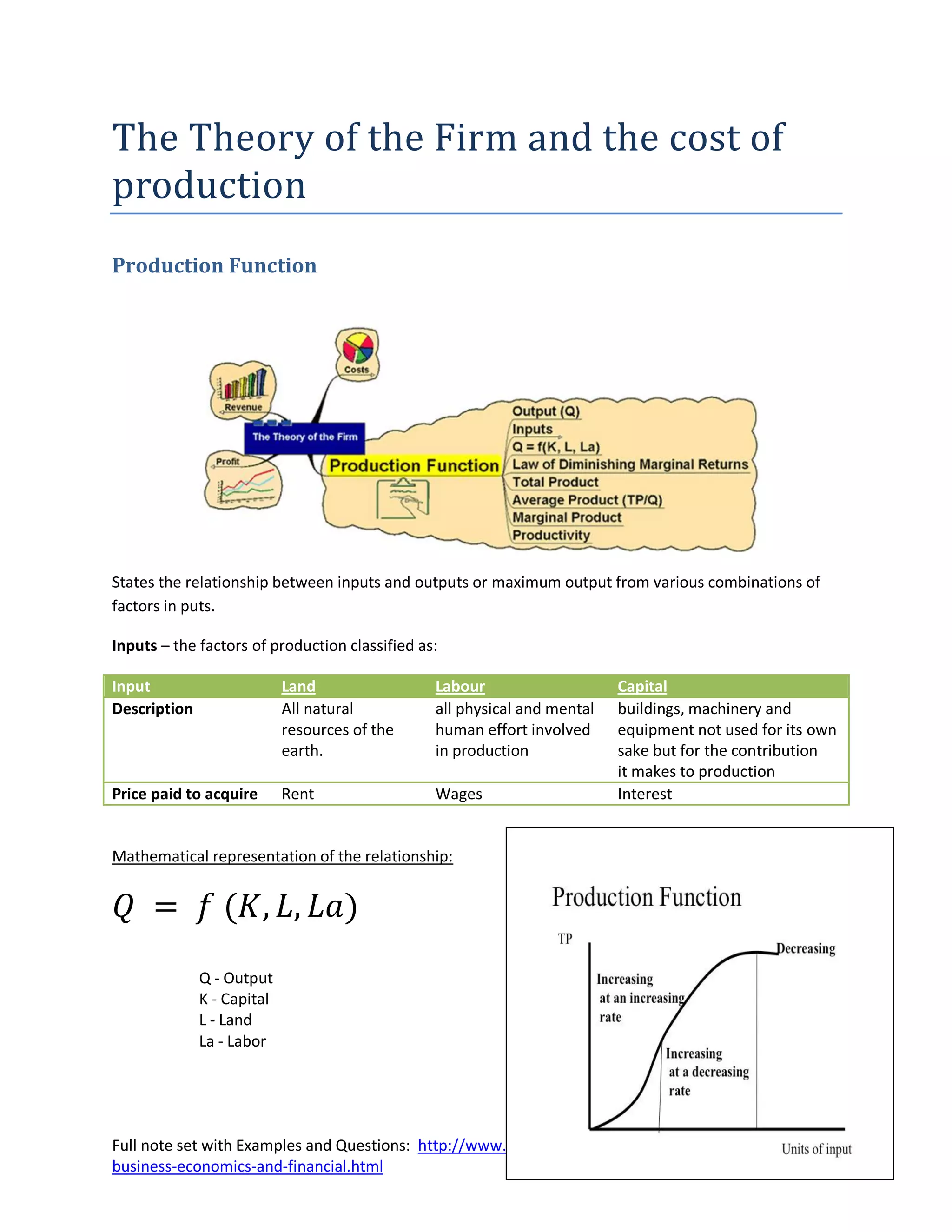
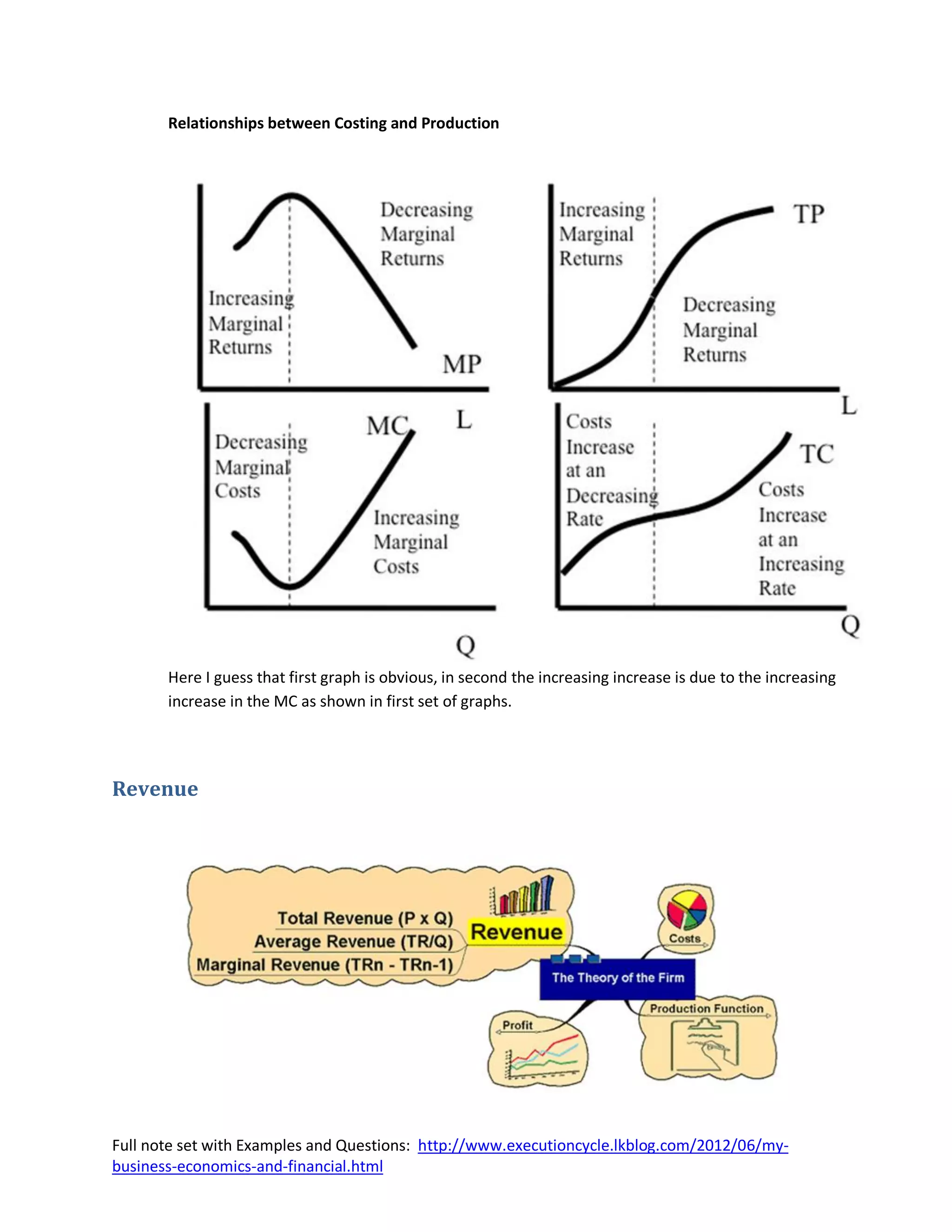
The document discusses the theory of the firm and the cost of production. It defines the production function as the relationship between inputs and outputs. It classifies inputs as land, labor, and capital. It then discusses the mathematical representation of the production function and analyzes production in the short run and long run. It also discusses concepts like marginal product, diminishing marginal returns, total cost, average cost, marginal cost, revenue, and profit.


![Lesson 9--production[1]](https://cdn.slidesharecdn.com/ss_thumbnails/lesson-9-production1-130409195935-phpapp02-thumbnail.jpg?width=640&height=640&fit=bounds)


![Coded Agents – with UiPath SDK + LangGraph [Virtual Hands-on Workshop]](https://cdn.slidesharecdn.com/ss_thumbnails/codedagentsdeck-251215155422-5497c599-thumbnail.jpg?width=640&height=640&fit=bounds)


