This document contains lecture notes for a course on principles of programming languages. It covers topics related to functional programming including expressions, procedures, recursion, types, and evaluators. It also briefly introduces logic programming and imperative programming concepts. The notes were prepared by Mira Balaban for a class at Ben-Gurion University with help from several teaching assistants.
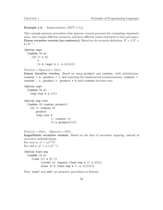
![Chapter 1
Functional Programming I – The
Elements of Programming
Functional Programming is a paradigm of programming that is most similar to evalua-tion
of expressions in mathematics. In functional programming a program is viewed as an
expression, which is evaluated by successive applications of functions to their arguments, and
substitution of the result for the functional expression. Its origin is in the lambda calculus
of Church.
The most characteristic feature of functional programming is the lack of state during a
computation. That is, a computation is not a sequence of states, created by triggers that
modify the states. Rather, a computation is a sequence of expressions, that result from
the successive evaluation of sub-expressions. Computation in functional programming has
no side-effects, because there are no variables to be assigned. That is, the only result of a
functional computation is the computed value, and there are no additional changes that can
take place during computation. Variables in functional programming denote values, rather
than locations, as in other kinds of programming (imperative programming). Functional
programming does not include a notion of variable assignment.
We concentrate on functional programming because it is a small and powerful paradigm
for introducing fundamental subjects and techniques in teaching programming languages.
Sources: SICP [1] 1.1, 1.2, 1.3 (online version http://deptinfo.unice.fr/~roy/sicp.pdf);
HTDP [2] 2.5. (online version http://htdp.org/2003-09-26/Book/)
Topics:
1. The elements of programming. SICP 1.1.1-3, 1.1.6.
2. Types in Scheme.
3. Program design: Writing contracts. HTDP 2.5.
4](https://image.slidesharecdn.com/principlesofprogramminglanguages-140901163422-phpapp01/85/Principles-of-programming-languages-9-320.jpg)

![Chapter 1 Principles of Programming Languages
’5
5
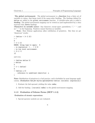
Explain!
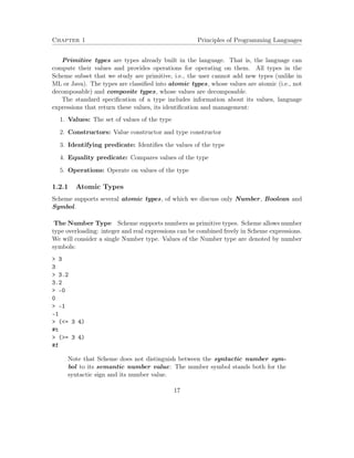
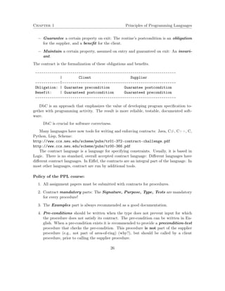
3. quote is a special operator. Its parameter is any sequence of characters (apart of
few punctuation symbols). It has a special evaluation rule: It returns its argument
as is – no evaluation. This differs from the evaluation rule for primitive procedures
(like symbol? and eq?) and the evaluation rule for compound procedures, which first
evaluate their operands, and then apply.
Question: What would have been the result if the operand of quote was evaluated
as for primitive procedures?
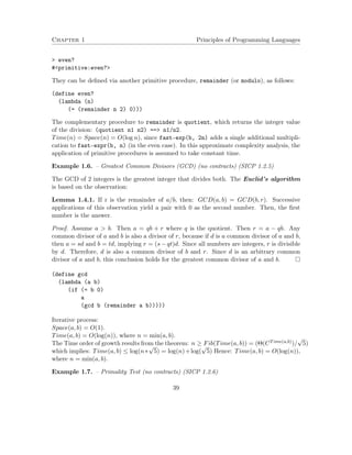
1.2.2 Composite Types
A composite type is a type whose values are composed from values of other types (including
self values, in the case of a recursive type). The values of a composite type can be decomposed
into values of other (or self) types. For example, the rational numbers can be viewed as the
composite Rational-number type, whose values are constructed, each, from two integer
values (and therefore, can be decomposed into their nominator and denominator integer
components). In the Scheme subset used in this course, the composite types are Procedure,
Pair and List. The latter two are introduced in chapter 3.
In order to describe a composite type we need to describe how values of the compo-nent
types are composed. This is achieved by using a type constructor which describes
type composition. Tuple composite types are described using the type constructor *, and
Procedure composite types are described using the type constructor -.
Example 1.1.
The type expression Number*Number*Boolean describes the set (type) of all triplets
of 2 numbers and a boolean, e.g., h2; 7:4;#ti; h0;63;#fi.
The type expression [Number – Number] describes the set of all single variable pro-cedures
(closures and primitive) from numbers to numbers. For example, the primitive
procedure abs (absolute value) and the closure hclosure (x) (+ x 1)i belong to this
type.
The type expression [Number*Boolean – Number] describes the set of all 2-variable
procedures from a number and a boolean to numbers.
The type expression Symbol*[Number – Number] describes the set of all pairs of a
symbol and a single variable procedure from numbers to numbers. For example, the
pairs h’abs primitive_abs_codei and h’square hclosure (x) (* x x)ii belong
to this type.
20](https://image.slidesharecdn.com/principlesofprogramminglanguages-140901163422-phpapp01/85/Principles-of-programming-languages-25-320.jpg)
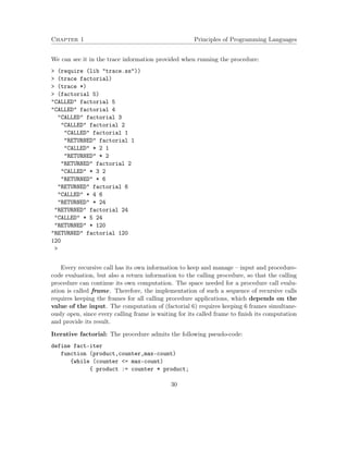
![Chapter 1 Principles of Programming Languages
The Procedure Type
The Procedure type is the set of all Scheme closures and primitive procedures. The type
is described using the type constructor -, and its closure values are created by the value
constructor lambda forms.
In order to assign a type to Scheme expressions that denote closures (lambda expressions)
we observe the types of their parameters and returned results. These can be inferred by
observing the expressions in the body of the lambda expressions.
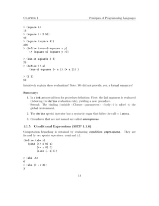
Example 1.2.
The type of (lambda (x) (+ (* x x) 3)) is [Number – Number]. This is deter-mined
from the known types of the primitive procedures +, *.
The type of (lambda (x y) (not (and x y))) is [T1*T2 – Boolean]. This is de-termined
from the known types of the primitive procedure not and the special operator
and1.
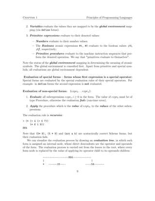
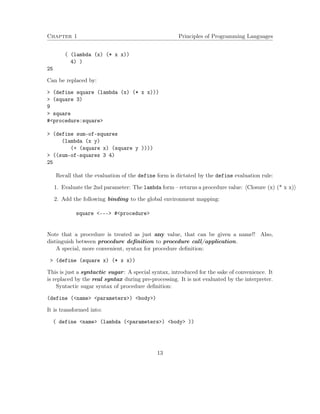
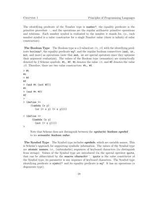
But, what is the type of the lambda expressions (lambda (x) x) (which creates the
identity procedure) and (lambda (f x) (f (f x)))? Evaluation of these expressions cre-ates
the closures hclosure (x) xi (the identity procedure) and hclosure (f x) (f (f x))i.
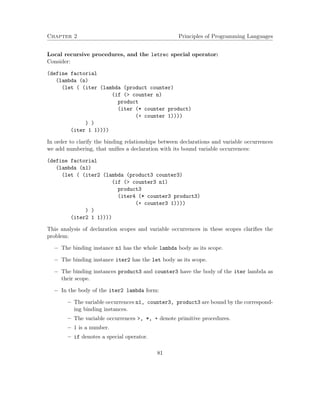
But to which types these closures belong? There are no primitive procedures or special oper-ators
to give us a hint. Observing their application we see that they apply well to arguments
of multiple types:
((lambda (x) x) 3)
3
((lambda (x) x) #t)
#t
((lambda (x) x) (lambda (x) (- x 1)))
#procedure:x
((lambda (x) x) (lambda (x) x))
#procedure:x
( (lambda (f x) (f (f x)))
abs -3)
3
( (lambda (f x) (f (f x)))
(lambda (x) (* x x))
3)
81
1The T1, T2 type parameters are due to the lack of real Boolean type in Scehme. In other languages the
type of this procedure would be [Boolean*Boolean – Boolean].
21](https://image.slidesharecdn.com/principlesofprogramminglanguages-140901163422-phpapp01/85/Principles-of-programming-languages-26-320.jpg)
![Chapter 1 Principles of Programming Languages
Therefore, these closures can actually belong to multiple Procedure types, based on their
argument types. For example, the closure hclosure (x) xi can belong to the types
[Number – Number],
[Boolean – Boolean],
[[Number – Number] – [Number – Number]].
We say that procedures (primitive and closures) that can accept arguments of varying types
are polymorphic, i.e., have multiple types and the expressions that create these procedures
are polymorphic expressions.
In order to assign a single type expression to polymorphic language expressions (and
procedures) we introduce type variables, denoted T1, T2, .... Type variables in type
expressions range over all types. Type expressions that include type variables are called
polymorphic type expressions since they denote multiple types.
The type of the identity lambda expression and procedure is [T – T].
The type of the expression (lambda (f x) (f x)) is [[T1 – T2]*T1 – T2].
The type of the expression (lambda (f x) (f (f x))) is [[T – T]*T – T].
In sum, the type constructor of the Procedure type is -, the value constructor for the
closures is lambda, and the identifying predicate is procedure?.
(procedure? (lambda (x) x))
#t
(procedure? abs)
#t
(procedure? display)
#t
(procedure? 5)
#f
Summary: Informal Syntax and Semantics:
Syntax: There are 2 kinds of Scheme language expressions:
1. Atomic:
(a) Primitives:
Number symbols.
Boolean symbols: #t, #f.
Primitive procedure symbols.
(b) Non-primitives:
Variable symbols.
22](https://image.slidesharecdn.com/principlesofprogramminglanguages-140901163422-phpapp01/85/Principles-of-programming-languages-27-320.jpg)
![Chapter 1 Principles of Programming Languages
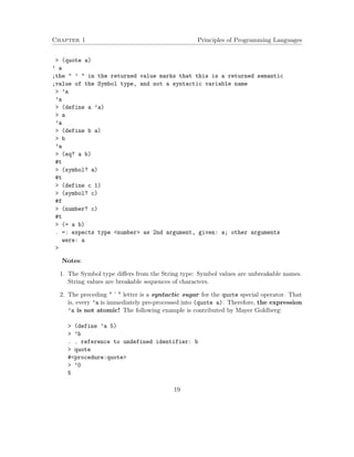
i. The set of all unbreakable keyboard character sequences. Includes vari-able
names.
ii. Value constructor: quote
iii. Identifying predicate: symbol?
Equality predicate: eq?
Operations: None (a degenerated type).
(b) Composite types:
Procedure:
i. A polymorphic type: The collection of all procedure (function) types.
Each concrete procedure type includes all procedures with the same
argument and result types.
ii. Type constructor: – written in infix notation. A Procedure type expres-sion
has the syntax: [ Type-expression-tuple – Type-expression].
Type expressions can be polymorphic, i.e., include type variables.
iii. Value constructor: For primitive procedures, their symbolic name is their
constructor. For user defined procedures (closures), lambda is the value
constructor.
iv. Identifying predicates:
For primitive procedures: primitive? For User defined procedures (clo-sures):
procedure?
Equality predicate: none.(why?)
Operations: All high order procedures (primitive and user defined).
1.3 Program Design Using Contracts
Following Felleison, Findler, Flatt and Krishnamurthi: How to Design Programs
http://www.htdp.org/2003-09-26/Book/
A procedure design starts with a contract that includes:
1. Signature
2. Purpose
3. Type
4. Example
5. Pre-conditions
6. Post-conditions
7. Tests
24](https://image.slidesharecdn.com/principlesofprogramminglanguages-140901163422-phpapp01/85/Principles-of-programming-languages-29-320.jpg)
![Chapter 1 Principles of Programming Languages
8. Invariants
Signature, purpose and type are mandatory to all procedures. Examples are desirable.
Tests are mandatory for complex procedures. Pre/post-conditions and invariants are rel-evant
only if non-trivial (not vacuous).
Contract:
Signature: area-of-ring(outer,inner)
Purpose: To compute the area of a ring whose radius is
’outer’ and whose hole has a radius of ’inner’
Type: [Number * Number - Number]
Example: (area-of-ring 5 3) should produce 50.24
Pre-conditions: outer = 0, inner = 0, outer = inner
Post-condition: result = PI * outer^2 - PI * inner^2
Tests: (area-of-ring 5 3) == 50.24
Definition: [refines the header]
(define area-of-ring
(lambda (outer inner)
(- (area-of-disk outer)
(area-of-disk inner))))
In this implementation area-of-ring is a caller of area-of-disk.
The specification of Types, Pre-conditions and Post-conditions requires special
specification languages. The keyword result belongs to the specification language for
post-conditions.
1.3.1 The Design by Contract (DBC) approach:
DbC is an approach for designing computer software. It prescribes that software designers
should define precise verifiable interface specifications for software components based upon
the theory of abstract data types and the conceptual metaphor of business contracts. The
approach was introduced by Bertrand Meyer in connection with his design of the Eiffel object
oriented programming language and is described in his book Object-Oriented Software
Construction (1988, 1997).
The central idea of DbC is a metaphor on how elements of a software system collaborate
with each other, on the basis of mutual obligations and benefits. The metaphor comes
from business life, where a client and a supplier agree on a contract. The contract defines
obligations and benefits. If a routine provides a certain functionality, it may:
Impose a certain obligation to be guaranteed on entry by any client module that calls
it: The routine’s precondition – an obligation for the client, and a benefit for the
supplier.
25](https://image.slidesharecdn.com/principlesofprogramminglanguages-140901163422-phpapp01/85/Principles-of-programming-languages-30-320.jpg)
![Chapter 1 Principles of Programming Languages
5. Post-conditions are recommended whenever possible. They clarify what the proce-dure
guarantee to supply. Post-conditions provide the basis for tests.
Continue the area-of-ring example: The area-of-ring is a client (a caller ) of the area-of-disk
procedure. Therefore, it must consider its contract, to verify that it fulfills the necessary
pre-condition. Here is a contract for the area-of-disk procedure:
Signature: area-of-disk(radius)
Purpose: To compute the area of a disk whose radius is the
’radius’ parameter.
Type: [Number - Number]
Example: (area-of-disk 2) should produce 12.56
Pre-conditions: radius = 0
Post-condition: result = PI * radius^2
Tests: (area-of-disk 2) == 12.56
Definition: [refines the header]
(define area-of-disk
(lambda (radius)
(* 3.14 (* radius radius))))
Area-of-ring must fulfill area-of-disk precondition when calling it. Indeed, this can
be proved as correct, since both parameters of area-of-disk are not negative. The post
condition of area-of-ring is correct because the post-condition of area-of-disk guaran-tees
that the results of the 2 calls are indeed, PI outer2 and PI inner2, and the definition
of area-of-ring subtracts the results of these calls.
We expect that whenever a client routine calls a supplier routine the client routine
will either explicitly call a pre-condition test procedure, or provide an argument
for the correctness of the call!
We do not encourage a defensive programming style, where each procedure first tests
its pre-condition. This is the responsibility of the clients.
1.4 Procedures and the Processes they Generate (SICP 1.2)
Iteration in computing refers to a process of repetitive computations, following a single
pattern. In imperative programming languages (e.g., Java, C++, C) iteration is speci-fied
by loop constructs like while, for, begin-until. Iterative computations (loops) are
managed by loop variables whose changing values determine loop exit. Loop constructs
27](https://image.slidesharecdn.com/principlesofprogramminglanguages-140901163422-phpapp01/85/Principles-of-programming-languages-32-320.jpg)
![Chapter 1 Principles of Programming Languages
provide abstraction of the looping computation pattern. Iteration is a central computing
feature.
Functional languages like the Scheme part introduced in this chapter do not posses
looping constructs like while. The only provision for computation repetition is repeated
function application. The question asked in this section is whether iteration by function call
obtains the advantages of iteration using loop constructs, as in other languages. We show
that recursive function call mechanism can simulate iteration. Moreover, the conditions
under which function call simulates iteration can be syntactically identified: A computing
agent (interpreter, compiler) can determine, based on syntax analysis of a procedure body,
whether its application can simulate iteration.
For that purpose, we discuss the computational processes generated by procedures.
We distinguish between procedure expression – a syntactical notion, to process – a
semantical notion. Recursive procedure expressions can create iterative processes. Such
procedures are called tail recursive.
1.4.1 Linear Recursion and Iteration (SICP 1.2.1 )
Consider the computation of the factorial function. In an imperative language, it is
natural to use a looping construct like while, that increments a factorial computation until
the requested number is reached. In Scheme, factorial can be computed by the following
two procedure definitions:
Recursive factorial:
Signature: factorial(n)
Purpose: to compute the factorial of a number ’n’.
This procedure follows the rule: 1! = 1, n! = n * (n-1)!
Type: [Number - Number]
Pre-conditions: n 0, an integer
Post-condition: result = n!
Example: (factorial 4) should produce 24
Tests: (factorial 1) == 1
(factorial 4) == 24
(define factorial
(lambda (n)
(if (= n 1)
1
(* n (factorial (- n 1))))
))
Alternative: Iterative factorial
28](https://image.slidesharecdn.com/principlesofprogramminglanguages-140901163422-phpapp01/85/Principles-of-programming-languages-33-320.jpg)
![Chapter 1 Principles of Programming Languages
(define factorial
(lambda (n)
(fact-iter 1 1 n) ))
fact-iter:
Signature: fact-iter(product,counter,max-count)
Purpose: to compute the factorial of a number ’max-count’.
This procedure follows the rule:
counter = 1; product = 1;
repeat the simultaneous transformations:
product -- counter * product, counter -- counter + 1.
stop when counter n.
Type: [Number*Number*Number - Number]
Pre-conditions:
product, counter, max-count 0
product * counter * (counter + 1) * ... * max-count = max-count!
Post-conditions: result = max-count!
Example: (fact-iter 2 3 4) should produce 24
Tests: (fact-iter 1 1 1) == 1
(fact-iter 1 1 4) == 24
(define fact-iter
(lambda (product counter max-count)
(if ( counter max-count)
product
(fact-iter (* counter product)
(+ counter 1)
max-count))))
Recursion vs. iteration:
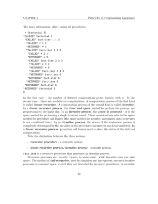
Recursive factorial: The evaluation of the form (factorial 6) yields the following se-quence
of evaluations:
(factorial 6)
(* 6 (factorial 5))
...
(* 6 (* 5 (...(* 2 factorial 1 )...)
(* 6 (* 5 (...(* 2 1)...)
...
(* 6 120)
720
29](https://image.slidesharecdn.com/principlesofprogramminglanguages-140901163422-phpapp01/85/Principles-of-programming-languages-34-320.jpg)
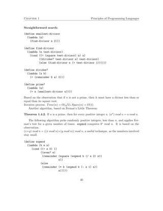
![Chapter 1 Principles of Programming Languages
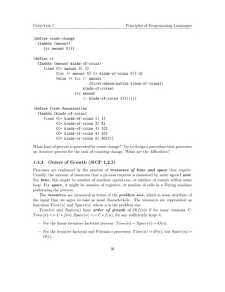
1.4.2 Tree Recursion (SICP 1.2.2)
Consider the following procedure definition for computing the n-th element in the sequence
of Fibonacci numbers:
Recursive FIB
Signature: (fib n)
Purpose: to compute the nth Fibonacci number.
This procedure follows the rule:
fib(0) = 0, fib(1) = 1, fib(n) = fib(n-1) + fib(n-2).
Type: [Number - Number]
Example: (fib 5) should produce 5
Pre-conditions: n = 0
Post-conditions: result = nth Fibonacci number.
Tests: (fib 3) == 2
(fib 1) == 1
(define fib
(lambda (n)
(cond ((= n 0) 0)
((= n 1) 1)
(else (+ (fib (- n 1))
(fib (- n 2)))))
))
The evaluation process generated by this procedure has a tree structure, where nested
forms lie on the same branch:
+-----------------(fib 5)----------------+
| |
+-----(fib 4)---------+ +-----(fib 3)---------+
| | | |
+--(fib 3)--+ +--(fib 2)-+ +-(fib 2)-+ (fib 1)
| | | | | | |
+-(fib 2)-+ (fib 1) (fib 1) (fib 0) (fib 1) (fib 0) 1
| | | | | | |
(fib 1) (fib 0) 1 1 0 1 0
1 0
The time required is proportional to the size of the tree, since the evaluation of (fib 5)
requires the evaluation of all fib forms. Hence, the time required is exponential in the
input of fib. The space required is proportional to the depth of the tree, i.e., linear in
34](https://image.slidesharecdn.com/principlesofprogramminglanguages-140901163422-phpapp01/85/Principles-of-programming-languages-39-320.jpg)
![Chapter 1 Principles of Programming Languages
the input.
Note: The exponential growth order applies to balanced (or almost balanced) trees. Highly
pruned computation trees can yield a smaller growth order.
Iterative FIB
(define fib
(lambda (n) (fib-iter 0 1 n)))
fib-iter:
Signature: fib-iter(current,next,count)
Purpose: to compute the nth Fibonacci number.
We start with current = 0, next = 1, and count as the Fibonacci goal,
and repeat the simultaneous transformation ’count’ times:
next -- next + current, current -- next,
in order to compute fib(count).
Type: [Number*Number*Number - Number]
Example: (fib-iter 0 1 5) should produce 5
Pre-conditions: next = (n+1)th Fibonacci number, for some n = 0;
current = nth Fibonacci number;
Post-conditions: result = (n+count)th Fibonacci number.
Tests: (fib-iter 1 2 3) == 5
(fib-iter 0 1 1) == 1
(define fib-iter
(lambda (current next count)
(if (= count 0)
current
(fib-iter next (+ current next) (- count 1)))
))
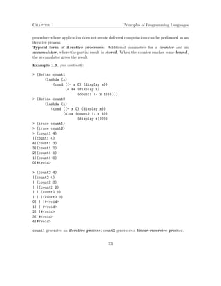
Example 1.4. – Counting Change (without contract)
Given an amount A of money, and types of coins (5 agorot, 10 agorot, etc), ordered in
some fixed way. Compute the number of ways to change the amount A. Here is a rule:
The number of ways to change A using n kinds of coins (ordered) =
number of ways to change A using the last n-1 coin kinds +
number of ways to change A - D using all n coin kinds, where D is the denomi-nation
of the first kind.
Try it!
35](https://image.slidesharecdn.com/principlesofprogramminglanguages-140901163422-phpapp01/85/Principles-of-programming-languages-40-320.jpg)
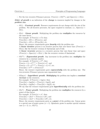
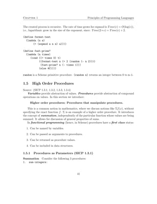
![Chapter 1 Principles of Programming Languages
Signature: sum-integers(a,b)
Purpose: to compute the sum of integers in the interval [a,b].
Type: [Number*Number - Number]
Post-conditions: result = a + (a+1) + ... + b.
Example: (sum-integers 1 5) should produce 15
Tests: (sum-integers 2 2) == 2
(sum-integers 3 1) == 0
(define sum-integers
(lambda (a b)
(if ( a b)
0
(+ a (sum-integers (+ a 1) b)))))
2. sum-cubes:
Signature: sum-cubes(a,b)
Purpose: to compute the sum of cubic powers of
integers in the interval [a,b].
Type: [Number*Number - Number]
Post-conditions: result = a^3 + (a+1)^3 + ... + b^3.
Example: (sum-cubes 1 3) should produce 36
Tests: (sum-cubes 2 2) == 8
(sum-cubes 3 1) == 0
(define sum-cubes
(lambda (a b)
(if ( a b)
0
(+ (cube a) (sum-cubes (+ a 1) b)))))
where cube is defined by: (define cube (lambda (x) (* x x x))).
3. pi-sum:
Signature: pi-sum(a,b)
Purpose: to compute the sum
1/(a*(a+2)) + 1/((a+4)*(a+6)) + 1/((a+8)*(a+10)) + ...
(which converges to PI/8, when started from a=1).
Type: [Number*Number - Number]
Pre-conditions: if a b, a != 0.
Post-conditions:
42](https://image.slidesharecdn.com/principlesofprogramminglanguages-140901163422-phpapp01/85/Principles-of-programming-languages-47-320.jpg)
![Chapter 1 Principles of Programming Languages
result = 1/a*(a+2) + 1/(a+4)*(a+6) + ... + 1/(a+4n)*(a+4n+2),
a+4n = b, a+4(n+1) b
Example: (pi-sum 1 3) should produce 1/3.
Tests: (pi-sum 2 2) == 1/8
(pi-sum 3 1) == 0
(define pi-sum
(lambda (a b)
(if ( a b)
0
(+ (/ 1 (* a (+ a 2))) (pi-sum (+ a 4) b)))))
The procedures have the same pattern:
(define name
(lambda (a b)
(if ( a b)
0
(+ (term a)
(name (next a) b)))))
The 3 procedures can be abstracted by a single procedure, where the empty slots term
and next are captured by formal parameters that specify the term and the next
functions, and name is taken as the defined function sum:
sum:
Signature: sum(term,a,next,b)
Purpose: to compute the sum of terms, defined by term
in predefined gaps, defined by next, in the interval [a,b].
Type: [[Number - Number]*Number*[Number - Number]*Number - Number]
Post-conditions: result = (term a) + (term (next a)) + ... (term n),
where n = (next (next ...(next a))) = b,
(next n) b.
Example: (sum identity 1 add1 3) should produce 6,
where ’identity’ is (lambda (x) x)
Tests: (sum square 2 add1 2) == 4
(sum square 3 add1 1) == 0
(define sum
(lambda (term a next b)
(if ( a b)
0
43](https://image.slidesharecdn.com/principlesofprogramminglanguages-140901163422-phpapp01/85/Principles-of-programming-languages-48-320.jpg)
![Chapter 1 Principles of Programming Languages
(+ (term a)
(sum term (next a) next b)))))
Using the sum procedure, the 3 procedures above have different implementations (same
contracts):
(define sum-integers
(lambda (a b)
(sum identity a add1 b)))
(define sum-cubes
(lambda (a b)
(sum cube a add1 b)))
(define pi-sum
(lambda (a b)
(sum pi-term a pi-next b)))
(define pi-term
(lambda (x)
(/ 1 (* x (+ x 2)))))
(define pi-next
(lambda (x)
(+ x 4)))
Discussion: What is the advantage of defining the sum procedure, and defining the three
procedures as concrete applications of sum?
1. First, the sum procedure prevents duplications of the computation pattern of sum-ming
a sequence elements between given boundaries. Duplication in software is bad
for many reasons, that can be summarized by management difficulties, and lack of
abstraction – which leads to the second point.
2. Second, and more important, the sum procedure expresses the mathematical notion of
sequence summation. Having this notion, further abstractions can be formulated, on
top of it. This is similar to the role of interface in object-oriented languages.
Definite integral – Definition based on sum: Integral of f from a to b is approximated
by: [f(a + dx=2) + f(a + dx + dx=2) + f(a + 2dx + dx=2) + :::] dx for small values of dx.
The definite integral can be computed (approximated) by the procedure:
(define dx 0.005)
44](https://image.slidesharecdn.com/principlesofprogramminglanguages-140901163422-phpapp01/85/Principles-of-programming-languages-49-320.jpg)
![Chapter 1 Principles of Programming Languages
(define integral
(lambda (f a b)
(* (sum f (+ a (/ dx 2)) add-dx b)
dx)))
(define add-dx
(lambda (x) (+ x dx)))
For example:
(integral cube 0 1 0.01)
0.2499875
(integral cube 0 1 0.001)
0.249999875
True value: 1/4.
Sequence-operation – Definition based on sum:
Signature: sequence-operation(operation,start,a,b)
Purpose: to compute the repeated application of an operation on
all integers in the interval [a,b], where start is
the neutral element of the operation.
Type: [[Number*Number - Number]*Number*Number*Number - Number]
Pre-conditions: start is a neutral element of operation:
(operation x start) = x
Post-conditions:
result = if a = b: a operation (a+1) operation ... b.
if a b: start
Example: (sequence-operation * 1 3 5) is 60
Tests: (sequence-operation + 0 2 2) == 2
(sequence-operation * 1 3 1) == 1
(define sequence-operation
(lambda (operation start a b)
(if ( a b)
start
(operation a (sequence-operation operation start (+ a 1) b)))))
where operation stands for any binary procedure, such as +, *, -, and start stands for the
neutral (unit) element of operation, i.e., 0 for +, and 1 for *. For example:
(sequence-operation * 1 3 5)
45](https://image.slidesharecdn.com/principlesofprogramminglanguages-140901163422-phpapp01/85/Principles-of-programming-languages-50-320.jpg)


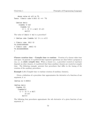
![Chapter 1 Principles of Programming Languages
Purpose: to construct a procedure that computes the average damp
of a function average-damp(f)(x) = (f(x) + x )/ 2
Type: [[Number - Number] - [Number - Number]]
Post-condition: result = closure r,
such that (r x) = (average (f x) x)
Tests: ((average-damp square) 10) == 55
((average-damp cube) 6) == 111
(define average-damp
(lambda (f)
(lambda (x) (average x (f x)))))
For example:
((average-damp (lambda (x) (* x x))) 10)
55
(average 10 ((lambda (x) (* x x)) 10))
55
((average-damp cube) 6)
111
(average 6 (cube 6))
111
(define av-damped-cube (average-damp cube))
(av-damped-cube 6)
111
Example 1.10. The derivative function:
For every number function, its derivative is also a function. The derivative of a function
can be created by a procedure generating procedure:
deriv:
Signature: deriv(f dx)
Purpose: to construct a procedure that computes the derivative
dx approximation of a function:
deriv(f dx)(x) = (f(x+dx) - f(x) )/ dx
Type: [[Number - Number]*Number - [Number - Number]]
Pre-conditions: 0 dx 1
Post-condition: result = closure r, such that
(r y) = (/ (- (f (+ x dx)) (f x))
dx)
Example: for f(x)=x^3, the derivative is the function 3x^2,
53](https://image.slidesharecdn.com/principlesofprogramminglanguages-140901163422-phpapp01/85/Principles-of-programming-languages-58-320.jpg)
![Chapter 1 Principles of Programming Languages
The problem is, of course, that once the condition does not evaluate to #f, the value of the
overall expression is the value of the consequence, even if the consequence value is #f. But
in this case the or operator evaluates the alternative. The or form can be corrected by
delaying the computation of the consequence and the alternative, using lambda abstraction:
(if condition consequence alternative) ==
((or (and condition (lambda () consequence)) (lambda () alternative)))
(if (zero? x) #f #t)
#f
((or (and (zero? x) (lambda () #f)) (lambda () #t)))
#f
Delayed computation for obtaining iterative processes Recall the distinction be-tween
recursive to iterative processes. A procedure whose computations are recursive is
characterized by a storage (frames in the Procedure-call stack) that stores the future com-putations,
once the recursion basis is computed. In Section 1.4 we provided iterative versions
for some recursive procedures. But they were based on new algorithms that compute the
same functions. In many cases this is not possible.
A recursive procedure can be turned iterative by using high order procedures that store
the delayed computations. These delayed computation procedures are created at run-time
and passed as arguments. Each delayed computation procedure corresponds to a frame in
the Procedure-call stack. The resulting iterative procedure performs the recursion base, and
calls itself with an additional delayed computation argument procedure.
Example 1.13. Turning the factorial recursive procedure iterative by using procedures that
store the delayed computations:
Consider the recursive factorial procedure:
Signature: factorial(n)
Purpose: to compute the factorial of a number ’n’.
This procedure follows the rule: 1! = 1, n! = n * (n-1)!
Type: [Number - Number]
Pre-conditions: n 0, an integer
Post-condition: result = n!
Example: (factorial 4) should produce 24
Tests: (factorial 1) == 1
(factorial 4) == 24
(define factorial
(lambda (n)
57](https://image.slidesharecdn.com/principlesofprogramminglanguages-140901163422-phpapp01/85/Principles-of-programming-languages-62-320.jpg)
![Chapter 2
Functional Programming II – Syntax,
Semantics and Types
Sources:
SICP [1] 1.1.5, 1.1.7, 1.3;
Krishnamurthi [8] 3, 24-26 (online version http://cs.brown.edu/~sk/Publications/Books/
ProgLangs/2007-04-26/plai-2007-04-26.pdf);
Friedman and Wand [3] 7 (online version: http://dl.taq.ir/computer/essentials_of_
programming_languages_friedman.pdf).
Topics:
1. Syntax: Concrete and Abstract.
2. Operational semantics: Applicative and Normal substitution models. SICP 1.1.5,
Krishnamurthi 3, SICP 1.1.7.
3. High order procedures revisited. SICP 1.3.
4. Type correctness: The type language; type correctness; type inference. Krishnamurthi
24-26, Friedman and Wand 7.
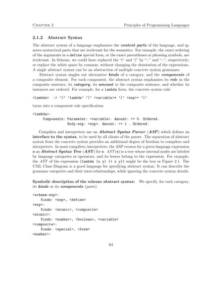
2.1 Syntax: Concrete and Abstract
Syntax of languages can be specified by a concrete syntax or by an abstract syntax.
The concrete syntax includes all syntactic information needed for parsing a language element
(program), e.g., punctuation marks. The abstract syntax include only the essential infor-mation
needed for language processing, e.g., for executing a program. The abstract syntax
is an abstraction of the concrete syntax: There can be many forms of concrete syntax for a
single abstract syntax. The abstract syntax provides a layer of abstraction that protects
against modifications of the concrete syntax.
61](https://image.slidesharecdn.com/principlesofprogramminglanguages-140901163422-phpapp01/85/Principles-of-programming-languages-66-320.jpg)
![Chapter 2 Principles of Programming Languages
2.1.1 Concrete Syntax:
The concrete syntax of a language defines the actual language. The concrete syntax of
Scheme is a small and simple context free grammar (Scheme is a context free language,
unlike most programming languages).
We use the BNF notation for specifying the syntax of Scheme. Quote from Wikipedia:
In computer science, Backus-Naur Form (BNF) is a metasyntax used to ex-press
context-free grammars: that is, a formal way to describe formal languages.
John Backus and Peter Naur developed a context free grammar to define the
syntax of a programming language by using two sets of rules: i.e., lexical rules
and syntactic rules.
BNF is widely used as a notation for the grammars of computer programming languages,
instruction sets and communication protocols, as well as a notation for representing parts
of natural language grammars.
1. Syntactic categories (non-terminals) are denoted as category.
2. Terminal symbols (tokens) are surrounded with ’.
3. Optional items are enclosed in square brackets, e.g. [item-x].
4. Items repeating 0 or more times are enclosed in curly brackets or suffixed with an
asterisk, e.g. word – letter letter*.
5. Items repeating 1 or more times are followed by a +.
6. Alternative choices in a production are separated by the | symbol, e.g.,
alternative-A j alternative-B.
7. Grouped items are enclosed in simple parentheses.
Concrete syntax of the subset of Scheme introduced so far:
scheme-exp - exp | ’(’ define ’)’
exp - atomic | ’(’ composite ’)’
atomic - number | boolean | variable
composite - special | form
number - Numbers
boolean - ’#t’ | ’#f’
variable - Restricted sequences of letters, digits, punctuation marks
special - lambda | quote | cond | if | let
form - exp+
define - ’define’ variable exp
62](https://image.slidesharecdn.com/principlesofprogramminglanguages-140901163422-phpapp01/85/Principles-of-programming-languages-67-320.jpg)
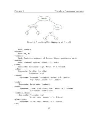
![Chapter 2 Principles of Programming Languages
Components: Predicate: exp
Consequence: exp
Alternative: exp
let:
Components: Var: variable-initialization. Amount: = 0.
Body: exp. Amount: = 1 . Ordered.
variable-initialization:
Components: Variable: variable
Expression: exp
The Scheme interpreters and compilers in chapter 4 use an abstract syntax based parser
for analyzing Scheme expressions. Figure 2.2 presents a UML class diagram [12, 9] for the
Scheme concrete syntax above.
Figure 2.2: Scheme Abstract Syntax formulated in UML class diagram
1. Categories are represented as classes.
2. Kinds are represented by class hierarchy relationships.
3. Components are represented as composition relationships between the classes.
2.2 Operational Semantics: The Substitution Model
The operational semantics is specified by a set of formal evaluation rules that can be
summarized as an algorithm eval(exp) for evaluation of Scheme expressions.
66](https://image.slidesharecdn.com/principlesofprogramminglanguages-140901163422-phpapp01/85/Principles-of-programming-languages-71-320.jpg)
![Chapter 2 Principles of Programming Languages
2.2.1 The Substitution Model – Applicative Order Evaluation:
The substitution model uses applicative order evaluation, which is an eager approach
for evaluation. The rules formalize the informally stated rules in Chapter 1:
1. Eval: Evaluate the elements of the compound expression;
2. Apply: Apply the procedure which is the value of the operator of the expression,
to the arguments, which are the values of the operands of the expression. For user
defined procedures (closures) this step is broken into 2 steps: substitute and reduce.
Therefore, the model is also called eval-substitute-reduce. The algorithm that defines the
operational semantics is called applicative-eval. It is a function:
applicative-eval: scheme-exp [ Scheme_type ! Scheme_type.
So far, Scheme_type = Number [ Boolean [ Symbol [ Procedure [ V oid [ Empty.
We use the predicates atom?, composite? number?, boolean?, and variable?, for
identifying atomic, composite, number, boolean, and variable expressions, respectively. The
predicates primitive-procedure?, and procedure? are used for identifying primitive pro-cedures
and user defined procedures, respectively. The predicate value? identifies Scheme
values, i.e., values in Scheme_type, that are created by evaluation of Scheme expressions.
The global environment value of a variable e is denoted GE(e). A variable-value pair
mapped by the global environment is called a binding, and denoted x; val . Addition
of a binding to the global environment, i.e., extending the GE mapping for a new variable x,
is denoted GE*x; val.
Signature: applicative-eval(e)
Purpose: Evaluate a Scheme expression
Type: [(scheme-exp union Scheme-type) - Scheme-type]
Definition:
applicative-eval[e] =
I. atom?(e):
1. number?(e) or boolean?( e):
applicative-eval[e] = e
2. variable?(e):
a. If GE(e) is defined:
applicative-eval[e] = GE(e)
b. Otherwise: e must be a variable denoting a Primitive procedure:
applicative-eval[e] = built-in code of e.
II. composite?(e): e = (e0 e1 ... en)(n = 0):
1. e0 is a Special Operator:
applicative-eval[e] is defined by the special evaluation rules
of e0 (see below).
70](https://image.slidesharecdn.com/principlesofprogramminglanguages-140901163422-phpapp01/85/Principles-of-programming-languages-75-320.jpg)
![Chapter 2 Principles of Programming Languages
2. a. Evaluate: compute applicative-eval[ei] = ei’ for i=0..n.
b. primitive-procedure?(e0’):
applicative-eval[e] = system application e0’(e1’, ..., en’).
c. procedure?(e0’):
e0’ is a closure: Closure (x1 ... xn) b1 ... bm
i. Substitute (preceded by renaming):
b1, ..., bm {x1 = e1’, ..., xn = en’} = b1’, ..., bm’
ii. Reduce: applicative-eval[b1’], ..., applicative-eval[b(m-1)’].
applicative-eval[e] = applicative-eval[bm’].
III. value?(e): applicative-eval[e] = e
Special operators evaluation rules:
1. e = (define x e1):
GE = GE*x, applicative-eval[e1]
2. e = (lambda (x1 x2 ... xn) b1 ... bm) at least one bi is required:
applicative-eval[e] = Closure (x1 ...xn) b1 ... bm
3. e = (quote e1):
applicative-eval[e] = e1
4. e = (cond (p1 e11 ...) ... (else en1 ...)):
If not(false?(applicative-eval[p1])):
applicative-eval[e11], applicative-eval[e12], ...
applicative-eval[e] = applicative-eval[last e1i]
Otherwise, continue with p2 in the same way.
If for all pi-s applicative-eval[pi] = #f:
applicative-eval[en1], applicative-eval[en2], ...
applicative-eval[e] = applicative-eval[last eni]
5. e = (if p con alt):
If true?(applicative-eval[p]):
then applicative-eval[e] = applicative-eval[con]
else applicative-eval[e] = applicative-eval[alt]
Note: value?(e) holds for all values computed by applicative-eval, i.e., for numbers,
boolean values (#t, #f), symbols (computed by the Symbol value constructor quote), and
closures (computed by the Procedure value constructor lambda).
Example 2.2. Recall the definitions from Chapter 1:
(define square (lambda (x) (* x x)))
(define sum-of-squares (lambda (x y)
71](https://image.slidesharecdn.com/principlesofprogramminglanguages-140901163422-phpapp01/85/Principles-of-programming-languages-76-320.jpg)
![Chapter 2 Principles of Programming Languages
(+ (square x) (square y))
))
(define f (lambda (a)
(sum-of-squares (+ a 1) (* a 2) )
))
Apply applicative-eval to the expression (f 5), assuming that these definitions are al-ready
evaluated.
(f 5)
136
applicative-eval[ (f 5) ] ==
applicative-eval[ f ] ==
Closure (a) (sum-of-squares (+ a 1) (* a 2) )
applicative-eval[ 5 ] == 5
==
applicative-eval[ (sum-of-squares (+ 5 1) (* 5 2)) ] ==
applicative-eval[sum-of-squares] ==
Closure (x y) (+ (square x) (square y))
applicative-eval[ (+ 5 1) ] ==
applicative-eval[ + ] == primitive-procedure +
applicative-eval[ 5 ] == 5
applicative-eval[ 1 ] == 1
== 6
applicative-eval[ (* 5 2) ] ==
applicative-eval[ * ] == primitive-procedure *
applicative-eval[ 5 ] == 5
applicative-eval[ 2 ] == 2
== 10
==
applicative-eval[ (+ (square 6) (square 10)) ] ==
applicative-eval[ + ] == primitive-procedure +
applicative-eval[ (square 6) ] ==
applicative-eval[ square ] == Closure (x) (* x x)
applicative-eval[ 6 ] == 6
==
applicative-eval[ (* 6 6) ] ==
applicative-eval[ * ] == primitive-procedure *
applicative-eval[ 6 ] == 6
applicative-eval[ 6 ] == 6
72](https://image.slidesharecdn.com/principlesofprogramminglanguages-140901163422-phpapp01/85/Principles-of-programming-languages-77-320.jpg)
![Chapter 2 Principles of Programming Languages
== 36
applicative-eval[ (square 10) ]
applicative-eval[ square ] == Closure (x) (* x x))
applicative-eval[ 10 ] == 10
==
applicative-eval[ (* 10 10) ] ==
applicative-eval[ * ] == primitive-procedure *
applicative-eval[ 10 ] == 10
applicative-eval[ 10 ] == 10
== 100
== 136
Example 2.3. A procedure with no formal parameters, and with a primitive expression as
its body:
(define five (lambda () 5))
five
Closure () 5
(five)
5
applicative-eval[ (five) ] ==
applicative-eval[ five ] == Closure () 5)
==
applicative-eval[ 5 ] ==
5
Example 2.4.
(define four 4)
four
4
(four)
ERROR: Wrong type to apply: 4
; in expression: (... four)
; in top level environment.
applicative-eval[ (four) ] ==
applicative-eval[ four ] == 4
the Evaluate step yields a wrong type.
73](https://image.slidesharecdn.com/principlesofprogramminglanguages-140901163422-phpapp01/85/Principles-of-programming-languages-78-320.jpg)
![Chapter 2 Principles of Programming Languages
Example 2.5.
(define y 4)
(define f (lambda (g)
(lambda (y) (+ y (g y)))))
(define h (lambda (x) (+ x y)))
(f h)
Closure (y1) (+ y1 ((lambda (x) (+ x y))
y1))
( (f h) 3)
10
applicative-eval[ (f h) ] ==
applicative-eval[ f ] ==
Closure (g) (lambda (y) (+ y (g y)))
applicative-eval[ h ] ==
Closure (x) (+ x y)
==
Substitute – rename both expressions and replace:
(lambda (y2) (+ y2 (g y2))){g = Closure (x1) (+ x1 y)}
==
applicative-eval[ (lambda (y2) (+ y2
(Closure (x1) (+ x1 y) y2 ) )) ]
==
Closure (y2) (+ y2 (Closure (x1) (+ x1 y) y2) )
Note the essential role of renaming here. Without it, the application ((f h) 3) would
replace all free occurrences of y by 3, yielding 9 as the result.
Example 2.6. Why is applicative-eval defined on Scheme-values, and not only on
Scheme expressions?
The values managed by applicative-eval are Numbers, booleans, symbols, and pro-cedures
– primitive or user defined. Number and Boolean values (semantics) are also
Number and Boolean expressions (syntax). Therefore, they do not need a separate seman-tic
formulation handling. In particular, as syntactic expressions they can be repeatedly
evaluated.
Values of the rest of the types are distinguished from their syntactic forms, and therefore,
cannot be repeatedly evaluated. Consider, for example, the following two evaluations:
74](https://image.slidesharecdn.com/principlesofprogramminglanguages-140901163422-phpapp01/85/Principles-of-programming-languages-79-320.jpg)
![Chapter 2 Principles of Programming Languages
applicative-eval[((lambda (x)(display x) x) (quote a))] ==
Eval:
applicative-eval[(lambda (x)(display x) x)] == Closure (x)(display x) x
applicative-eval[(quote a)] == the symbol ’a’
Substitute:
(display x), x {x = ’a’} = (display ’a’), ’a’
Reduce:
applicative-eval[ (display ’a’) ] ==
Eval:
applicative-eval[display] == Code of display.
applicative-eval[’a’] == ’a’ , since ’a’ is a value of the symbol (*)
type (and not a variable!).
applicative-eval[’a’] == ’a’
and also
((lambda (f x)(f x)) (lambda (x) x) 3)
3
applicative-eval[ ((lambda (f x)(f x)) (lambda (x) x) 3) ] ==
Eval:
applicative-eval[(lambda (f x)(f x))] == Closure (f x)(f x)
applicative-eval[(lambda (x) x) ] == Closure (x) x)
applicative-eval[3] == 3
Substitute following renaming:
(f1 x1){f1 = Closure (x2) x2, x1 = 3} = (Closure (x2) x2 3)
Reduce:
applicative-eval[(Closure (x2) x2 3)] ==
Eval:
applicative-eval[Closure (x2) x2] == Closure (x2) x2 (*)
applicative-eval[3] == 3
Substitute x2 by 3 in x2 == 3
Reduce:
applicative-eval[3]= 3
In both evaluations, values created by computation of applicative-eval (the symbol a
and the closure Closure (x2) x2, are repeatedly evaluated. The evaluation completes
correctly because applicative-eval avoids repetitive evaluations (the lines marked by (*).
Otherwise, the first evaluation would have failed with an “unbound variable” error, and the
second with “unknown type of argument”.
75](https://image.slidesharecdn.com/principlesofprogramminglanguages-140901163422-phpapp01/85/Principles-of-programming-languages-80-320.jpg)
![Chapter 2 Principles of Programming Languages
The substitution model – applicative order uses the call-by-value method
for parameter passing.
Parameter passing method: In procedure application, the values of the ac-tual
arguments are substituted for the formal parameters. This is the standard
evaluation model in Scheme (LISP), and the most frequent method in other
languages (Pascal, C, C++, Java).
2.2.2 The Substitution Model – Normal Order Evaluation:
applicative-eval implements the eager approach in evaluation. The eagerness is
expressed by immediate evaluation of arguments, prior to closure application. An alternative
algorithm, that implements the lazy approach in evaluation avoids argument evaluation
until essential:
1. Needed for deciding a computation branch.
2. Needed for application of a primitive procedure.
The normal-eval algorithm is similar to applicative-eval. The only difference, which
realizes the lazy approach, is moving the argument evaluation from step II.2.a. into step
II.2.b., just before a primitive procedure is applied. Otherwise, the algorithm is unchanged,
and the computation rules for the special operators are the same:
Signature: normal-eval(e)
Purpose: Evaluate a Scheme expression
Type: [scheme-exp - Scheme-type]
Definition:
normal-eval[e] =
I. atom?(e):
1. number?(e) or boolean?( e):
applicative-eval[e] = e
2. variable?(e):
a. If GE(e) is defined:
applicative-eval[e] = GE(e)
b. Otherwise: e must be a variable denoting a Primitive procedure:
applicative-eval[e] = built-in code of e.
II. (composite? e): e = (e0 e1 ... en)(n = 0):
1. e0 is a Special Operator:
normal-eval[e] is defined by the special evaluation rules of e0.
2. a. Evaluate: compute normal-eval[e0] = e0’.
b. (primitive-procedure? e0’):
Evaluate: compute normal-eval[ei] = ei’ for all ei.
normal-eval[e] = system application e0’(e1’, ..., en’).
76](https://image.slidesharecdn.com/principlesofprogramminglanguages-140901163422-phpapp01/85/Principles-of-programming-languages-81-320.jpg)
![Chapter 2 Principles of Programming Languages
c. (procedure? e0’):
e0’ is a closure: Closure (x1 ... xn) b1 ... bm :
i. Substitute (preceded by renaming):
b1, ..., bm {x1 = e1, ..., xn = en} = b1’, ..., bm’
ii. Reduce: normal-eval[b1’], ..., normal-eval[bm’]
iii. Return: normal-eval[e] = normal-eval[bm’]
Note that normal-eval is defined only on Scheme expressions (as expected from an inter-preter).
Why?
Example 2.7. The Expansions step – In this step there are no evaluations, just replace-ments.
normal-eval[ (f 5) ] ==
normal-eval[f] == Closure (a) (sum-of-squares (+ a 1) (* a 2))
==
normal-eval[ (sum-of-squares (+ 5 1) (* 5 2)) ] ==
normal-eval[ sum-of-squares ] ==
Closure (x y) (+ (square x) (square y))
==
normal-eval[ (+ (square (+ 5 1)) (square (* 5 2))) ] ==
normal-eval[ + ] == primitive-procedure +
normal-eval[ (square (+ 5 1)) ] ==
normal-eval[ square ] == Closure (x) (* x x)
==
normal-eval[ (* (+ 5 1) (+ 5 1)) ] ==
normal-eval[ * ] == primitiv-procedure *
normal-eval[ (+ 5 1) ] ==
normal-eval[ + ] == primitive-procedure +
normal-eval[ 5 ] == 5
normal-eval[ 1 ] == 1
== 6
normal-eval[ (+ 5 1) ] ==
normal-eval[ + ] == primitive-procedure +
normal-eval[ 5 ] == 5
normal-eval[ 1 ] == 1
== 6
== 36
normal-eval[ (square (* 5 2)) ] ==
normal-eval[ square ] == Closure (x) (* x x)
==
77](https://image.slidesharecdn.com/principlesofprogramminglanguages-140901163422-phpapp01/85/Principles-of-programming-languages-82-320.jpg)
![Chapter 2 Principles of Programming Languages
normal-eval[ (* (* 5 2) (* 5 2)) ] ==
normal-eval[ * ] == primitiv-procedure *
normal-eval[ (* 5 2) ] ==
normal-eval[ * ] == primitive-procedure *
normal-eval[ 5 ] == 5
normal-eval[ 2 ] == 2
== 10
normal-eval[ (* 5 2) ] ==
normal-eval[ * ] == primitive-procedure *
normal-eval[ 5 ] == 5
normal-eval[ 2 ] == 2
== 10
== 100
== 136
2.2.3 Comparison: The applicative order and the normal order of evalu-ations:
1. If both orders terminate (no infinite loop): They compute the same value.
2. Normal order evaluation repeats many computations.
3. Whenever applicative order evaluation terminates, normal order terminates as well.
4. There are expressions where normal order evaluation terminates, while applicative
order does not:
(define f (lambda (x) (f x)))
(define g (lambda (x) 5))
(g (f 0))
In normal order, the application (f 0) is not reached. In applicative order: Better,
do not try! Most interpreters use application-order evaluation.
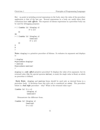
5. Side effects (like printing – the display primitive in Scheme) can be used to detect
the evaluation order. Consider, for example,
(define f (lambda (x) (display x) (newline) (+ x 1)))
(define g (lambda (x) 5))
(g (f 0))
0
5
78](https://image.slidesharecdn.com/principlesofprogramminglanguages-140901163422-phpapp01/85/Principles-of-programming-languages-83-320.jpg)
![Chapter 2 Principles of Programming Languages
What evaluation order was used?
What are the side effect and the result in the other evaluation order?
Explain the results by applying both evaluation orders of the eval algorithm.
The normal-order evaluation model uses the call-by-name method for param-eter
passing: In procedure application, the actual arguments themselves are
substituted for the formal parameters. This evaluation model is used in Scheme
(LISP) for special forms. The call be name method was first introduced in
Algol-60.
2.2.4 High Order Functions Revisited
Recall the special operator let, which is a syntactic sugar for application of an anonymous
lambda, i.e., runtime creation of a closure and its immediate application. For example, the
procedure
(define f
(lambda ( x y)
(let ((a (+ 1 (* x y)))
(b (- 1 y)))
(+ (* x (square a))
(* y b)
(* a b)))))
is actually the procedure:
(define f
(lambda (x y)
((lambda (a b)
(+ (* x (square a))
(* y b)
(* a b)))
(+ 1 (* x y))
(- 1 y))
))
Therefore:
applicative-eval[ (f 3 1) ] ==*
Substitute: body of f{x = 3, y = 1} ==
79](https://image.slidesharecdn.com/principlesofprogramminglanguages-140901163422-phpapp01/85/Principles-of-programming-languages-84-320.jpg)
![Chapter 2 Principles of Programming Languages
applicative-eval[ ((lambda (a b) (+ (* 3 (square a))
(* 1 b)
(* a b)))
(+ 1 (* 3 1))
(- 1 1)) ] ==*
applicative-eval[ (+ (* 3 16) (* 1 0) (* 4 0)) ] ==
48
The symbol ==* is used to denote application of several applicative-eval steps.
2.2.4.1 Defining local procedures
Can we use let for defining local variables whose value is a procedure?
(define f
(lambda (x y)
(let ( (f-helper (lambda (a b)
(+ (* x (square a))
(* y b)
(* a b)))
) )
(f-helper (+ 1 (* x y))
(- 1 y)))
))
applicative-eval[ (f 3 1) ] ==
applicative-eval[ f ] == Closure (x y) (let ...)
applicative-eval[ 3 ] == 3
applicative-eval[ 1 ] == 1
Substitute: body of f{x = 3, y = 1} ==
applicative-eval[ ( (lambda (f-helper) (f-helper (+ 1 (* 3 1))
(- 1 1)))
(lambda (a b)(+ (* 3 (square a))
(* 1 b)
(* a b))) ) ] ==*
applicative-eval[ ( Closure (a b)(+ (* 3 (square a))
(* 1 b)
(* a b))
(+ 1 (* 3 1))
(- 1 1)) ] ==*
applicative-eval[ (+ (* 3 16) (* 1 0) (* 4 0)) ] ==*
48
80](https://image.slidesharecdn.com/principlesofprogramminglanguages-140901163422-phpapp01/85/Principles-of-programming-languages-85-320.jpg)
![Chapter 2 Principles of Programming Languages
– iter4 is a free variable!!!!! Causes a runtime error in evaluation:
applicative-eval[ (factorial 3) ] ==*
Substitute: body of factorial{n = 3} ==
applicative-eval[ ( (lambda (iter) (iter 1 1))
(lambda (product counter)
(if ( counter 3)
product
(iter (* counter product)
(+ counter 1))))
) ] ==*
applicative-eval[ ( Closure (product counter)
(if ( counter 3)
product
(iter (* counter product)
(+ counter 1)))
1 1) ] ==*
applicative-eval[ (if ( 1 3) 1 (iter (* 1 1) (+ 1 1))) ] ==*
applicative-eval[ (iter (* 1 1) (+ 1 1)) ] ==
*** RUN-TIME-ERROR: variable iter undefined ***
The problem is that iter is a recursive procedure: It applies the procedure iter which
is not globally defined. iter is just a parameter that was substituted by another procedure.
Once iter is substituted, its occurrence turns into a free variable, that must be already
bound when it is evaluated. But, unfortunately, it is not! This can be seen clearly, if we
replace the let abbreviation by its meaning expression:
1. (define factorial
2. (lambda (n)
3. ( (lambda (iter) (iter 1 1))
4. (lambda (product counter)
5. (if ( counter n)
6. product
7. (iter (* counter product)
8. (+ counter 1))))
9. )))
(factorial 3)
reference to undefined identifier: iter
82](https://image.slidesharecdn.com/principlesofprogramminglanguages-140901163422-phpapp01/85/Principles-of-programming-languages-87-320.jpg)


![Chapter 2 Principles of Programming Languages
2.2.5 Function Currying
Currying is a technique for turning a function (procedure) of n parameters into a chain of n
single parameter procedures. It is called after Haskell Curry. It is used when parameters are
not all available, and fixing part of them enables partial evaluation of a procedure code.
Currying turns a procedure (lambda (x1 x2 ... xn) body) into a chain of high order
procedures (lambda (x1) (lambda (x2) ... (lambda (xn) body)...)). The Currying
technique is used in every language that supports closures, i.e., run-time created procedures:
All functional languages, Javascript, C#.
Example 2.9.
Signature: add(x,y)
Type: [Number*Number - Number]
(define add
(lambda (x y) (+ x y)))
Can be Curried into:
Signature: c-add(x)
Type: [Number - [Number - Number]]
(define c-add
(lambda (x)
(lambda (y) (add x y))))
(define add3 (c-add 3))
(add3 4)
7
Example 2.10. Recall the sum procedure for summing finite sequences:
Signature: sum(term a next b)
Type: [[Number - Number]*Number*[Number - number]*Number -Number]
(define sum
(lambda (term a next b)
(if ( a b)
0
(+ (term a)
(sum term (next a) next b)))))
For a given mathematical sequence, the procedures term, next are fixed and maybe fre-quently
used for varying intervals. In that case, sum can be Curried into c-sum and reused
for multiple interval boundaries:
86](https://image.slidesharecdn.com/principlesofprogramminglanguages-140901163422-phpapp01/85/Principles-of-programming-languages-91-320.jpg)
![Chapter 2 Principles of Programming Languages
Signature: c-sum(term)
Type: [[Number - Number] - [[Number - number] - [Number*Number -Number]]]
(define c-sum
(lambda (term)
(lambda (next)
(lambda (a b)
(sum term a next b)))))
For the sequence of squares with skips of 2:
ha2; (a + 2)2; :::i :
(define sum-sqrts-skip2 ((c-sum (lambda (x)(* x x)))
(lambda (x) (+ x 2)) ))
(sum-sqrts-skip2 2 6)
56
Further generalization can involve general Currying procedures:
Signature: curry2(f)
Type: [[T1*T2 - T3] - [T1 - [T2 - T3]]]
(define curry2
(lambda (f)
(lambda (x)
(lambda (y) (f x y)))))
(((curry2 add) 3) 4)
7
(define add3 ((curry2 add) 3))
(add3 4)
7
(add3 7)
10
Example 2.11 (Naive Currying).
Consider a more complex version of the add procedure, where a complex computation,
say the recursive fib procedure, is applied to the available (non-delayed) parameter:
Signature: add-fib(x,y)
Type: [Number*Number - Number]
(define add-fib
(lambda (x y)
(+ (fib x) y)))
(add-fib 4 5)
87](https://image.slidesharecdn.com/principlesofprogramminglanguages-140901163422-phpapp01/85/Principles-of-programming-languages-92-320.jpg)
![Chapter 2 Principles of Programming Languages
10
Naive Currying:
Signature: c-add-fib(x)
Type: [Number - [Number - Number]]
(define c-add-fib
(lambda (x)
(lambda (y)
(+ (fib x) y))))
(define add-fib4 (c-add-fib 4))
(add-fib4 5)
10
(add-fib4 3)
8
(add-fib4 5)
10
This Currying is naive because it does not meet the expectations of partial evaluation: In
every application of add-fib4, (fib 4) is re-computed, although we could have computed
it once at the time of Currying, i.e., before the definition of add-fib4.
The following version demonstrates the full idea of Currying: Delaying computations
in unknown variables, while applying computations in known variables.
(define c-add-fib
(lambda (x)
(let ((fib-x (fib x))) ;Applying known computation
(lambda (y) ;delaying unknown computations
(+ fib-x y)))
))
Using the new version, (fib 4) is computed once, while add-fib-4 is defined.
Example 2.12. Consider the recursive procedure expt:
Signature: expt(x,y)
Type: [Number*Number - Number]
(define expt
(lambda (b n)
(if (= n 0)
1
(* b (expt b (- n 1))))))
88](https://image.slidesharecdn.com/principlesofprogramminglanguages-140901163422-phpapp01/85/Principles-of-programming-languages-93-320.jpg)
![Chapter 2 Principles of Programming Languages
Naive Currying:
Signature: c-expt(x,y)
Type: [Number - [Number - Number]]
(define c-expt
(lambda (b)
(lambda (n)
(expt b n))))
((c-expt 3) 4)
81
Another naive Currying:
(define c-expt
(lambda (b)
(lambda (n)
(if (= n 0)
1
(* b ((c-expt b) (- n 1)) )))
))
Both Curried versions are naive since the Curried procedures still need to apply computations
or to handle substitutions of the known variable b. In order to cope with the recursion,
we define a local recursive procedure that resides in the scope of the known variable and
therefore does not need it as a parameter:
(define c-expt
(lambda (b)
(letrec ((helper (lambda (n)
(if (= n 0)
1
(* b (helper (- n 1)))))
))
helper
)))
(define expt3 (c_expt 3) )
(expt3 4)
81
expt3 is a procedure in the single delayed variable n, in which all occurrences of the known
variable b are already substituted.
Example 2.13.
89](https://image.slidesharecdn.com/principlesofprogramminglanguages-140901163422-phpapp01/85/Principles-of-programming-languages-94-320.jpg)

![Chapter 2 Principles of Programming Languages
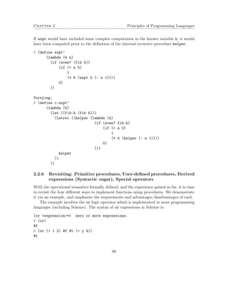
The let sub-expression is in head position.
The (+ 2 3) and 5 sub-expressions of the let expressions are in head positions.
The (f a b) sub-expression of the let expression is in tail position.
The 2 and 3 sub-expressions of (+ 2 3) are in head positions.
The f, a, b sub-expressions of (f a b) are in head positions.
An expression is in tail form if its head positions do not include calls to user procedures,
and its sub-expressions are in tail form. By default, atomic expressions are in tail form.
Example 2.15.
(+ 1 x) is in tail form.
(if p x (+ 1 (+ 1 x))) is in tail form.
(f (+ x y)) is in tail form.
(+ 1 (f x)) is not in tail form (but (f x) is in tail form).
(if p x (f (- x 1))) is in tail form.
(if (f x) x (f (- x 1))) is not in tail form.
(lambda (x) (f x)) is in tail form.
(lambda (x) (+ 1 (f x))) is not in tail form.
(lambda (x) (g (f 5))) is not in tail form.
Proposition 2.2.1. Expressions in tail form create iterative processes.
2.3 Type Correctness
Based on Krishnamurthi [8] chapters 24-26, Friedman and Wand [3] chapter 7.
Contracts of programs provide specification for their most important properties: Sig-nature,
type, preconditions and postconditions. It says nothing about the implementation
(such as performance).
Program correctness deals with proving that a program implementation satisfies its
contract:
1. Type correctness: Check well-typing of all expressions, and possibly infer missing
types.
95](https://image.slidesharecdn.com/principlesofprogramminglanguages-140901163422-phpapp01/85/Principles-of-programming-languages-100-320.jpg)
![Chapter 2 Principles of Programming Languages
procedure and function variables) must be provided with full typing information. Such are,
for example, the languages Java, C, C++, Pascal1.
Some languages have a partially typed syntax, i.e., programs do not necessarily asso-ciate
their constructs with types. The Scheme and Prolog languages do not include any typ-ing
information. The ML language allows for partial type specification. In such languages,
typing information might arise from built-in types of language primitives. For example,
in Scheme, number constants have the built-in Number type, and the arithmetic primitive
procedures “-” has the built-in Procedure type [Number*Number – Number].
If a language syntax does not include types, and there are no built-in primitives with
built-in types, then the language has an untyped semantics. Pure Logic Programming is
an untyped language.
Static/dynamic type checking/inference: Type checking/inference is performed by
an algorithm that uses type information within the program code for checking well typing
conditions. If the type checking algorithm is based only on the program code, then it can be
applied off-line, without actually running the program. This is static type checking/in-ference.
Such an algorithm uses the known semantics of language constructs for statically
checking well typing conditions. A weaker version of a type checking algorithm requires
concrete data for checking well typing, usually based on type tagging of values. There-fore,
they require an actual program run, and the type checking is done at runtime. This
is dynamic type checking. Clearly, static type checking is preferable over dynamic type
checking.
The programming languages Pascal, C, C++, Java that have a fully typed syntax, have
static type checking algorithms. The ML language, that allows for partial type specification,
has static type inference algorithms. That is, based on partial type information provided
for primitives and in the code, the algorithm statically infers type information, and checks
for well typing. The Scheme and Prolog languages, that have no type information in their
syntax, have only dynamic typing.
Properties of type checking/inference algorithms: The goal of a type checking/in-ference
algorithm is to detect all violations of well typing. A type checking algorithm that
detects all such violations is termed strong. Otherwise, it is weak. The difficulty is, of
course, to design efficient, static, strong type checking algorithms. Static type checkers need
to follow the operational semantics of the language, in order to determine types of expres-sions
in a program, and check for well typing. The type checker of the C language is known
to be weak, due to pointer arithmetics.
How types are specified? Specification of typing information in the program and within
type checking algorithms requires a language for writing types. A type specification language
1Java generics and C++ templates provide a restricted form of type variables.
97](https://image.slidesharecdn.com/principlesofprogramminglanguages-140901163422-phpapp01/85/Principles-of-programming-languages-102-320.jpg)
![Chapter 2 Principles of Programming Languages
(lambda (x y)
(if (= y 0)
’unspecified
(/ x y)))
returns either a symbol or a number. Its type is [Number*Number - Symbol union Number].
The set of values of a Union type is the union of the value sets of the argument types.
Union types are composite. They have no value constructors since their values are obtained
from their argument types. The type constructor for Union types is union. Simplification
of union type expressions:
1. The self union property: Since self union of sets has the property S [ S = S, we
introduce the simplification rule:
For every type expression TexpS:
Texp union TexpS is equal to TexpS, denoted TexpS union TexpS = TexpS.
The self union property enables the simplification of Number union Number into Number.
2. The commutativity property: Since set union is commutative, we introduce the
simplification rule:
For every type expressions TexpS1, TexpS2:
Texp1 union Texp2 is equal to Texp2 union Texp1, denoted Texp1 union Texp2 =
Texp2 union Texp1.
The commutativity and the self union properties enable the simplification of (Number
union Symbol) union (Symbol union Number) into Number union Symbol.
The Void type: What is the type of the procedure:
(lambda (x) (display x))) ; Bad style. Why?
Indeed this is a bad style programming since the returned value is that of a side effect
procedure display, i.e., unspecified in the semantics. Therefore, this procedure cannot
be embedded in composite expressions! However, it must be typed. The Void type that
denotes the singleton set fvoidg, is inserted for typing such expressions. The type of the
above procedure is: [T – Void].
The Tuple type: This type is introduced in order to account for procedures with any
number of parameters. This type describes n-tuple values. It includes the Empty type, that
describes 0-tuples, i.e., the empty set, and all tuple types T1 * ... * Tn, that stand for
n-tuple values. For every n, and every set of type expressions T1, ..., Tn, the expression
T1 * ... * Tn describes a tuple type. For example, Number * Boolean describes all 2-
tuples of a number and a boolean values. The symbol * is the type constructor of n-tuple
types, for n0.
99](https://image.slidesharecdn.com/principlesofprogramminglanguages-140901163422-phpapp01/85/Principles-of-programming-languages-104-320.jpg)
![Chapter 2 Principles of Programming Languages
The parameter type of all procedures is Tuple. The parameter type of parameter-less
procedures is Empty. For example, the type of the procedure: (lambda () 5) is [Empty –
Number]. Procedures with n parameters have an n-tuple type as their parameter type. For
example, the parameter type of the procedure (lambda (x y) 5) is T1 * T2.
The Scheme subset introduced so far does not include tuple values. That is, no value
constructors for tuples have been introduced. In Chapter 3, we will introduce the Pair
type, with its value constructor cons.
Type polymorphism in Scheme: Scheme expressions that do not include primitives do
not have a specified type. Such expressions can yield, at runtime, values of different types,
based on the types of their variables. For example, the procedure:
(lambda (x) x)
can be applied to values of any type and returns a value of the input type:
( (lambda (x) x) 3)
3
( (lambda (x) x) #t)
#t
( (lambda (x) x) (lambda (x) (+ x 1)))
#procedure:x
Therefore, the identity procedure has multiple types in these applications:
In the first: [Number – Number]
In the 2nd: [Boolean – Boolean]
In the 3rd: [[Number – Number] – [Number – Number]]
We see that a single procedure expression has multiple types – based on its application. In
order to describe its type by a single expression, we introduce type variables to the type
specification language – denoted as T, T1, T2, ...:
1. The type expression that describes the types of the identity procedure is [T – T].
2. The type expression that describes the type of (lambda (f x) (f x)) is [[T1 -
T2]*T1 - T2].
3. The type expression that describes the type of (lambda (f x) ( (f x) x)) is [[T1
- [T1 - T2]]*T1 - T2].
Terminology:
Polymorphic type expressions: Type expressions that include type variables are
called polymorphic type expressions. They describe multiple concrete types.
100](https://image.slidesharecdn.com/principlesofprogramminglanguages-140901163422-phpapp01/85/Principles-of-programming-languages-105-320.jpg)
![Chapter 2 Principles of Programming Languages
Instantiation (substitution) of type variables: Type variables within a type ex-pression
have a bound status, and therefore, can be consistently substituted. The
substitution yields instances of the original type expression. For example, the Pro-cedure
types:
[Number - Number]
[Symbol - Symbol]
[[Number - Number] - [Number - Number]]
[[Number - T1] - [Number - T1]]
are instances of the polymorphic type expression:
[T - T]
A polymorphic type expression describes (is an abstraction of) its instance type ex-pressions.
Polymorphic type constructors: A type constructor that can create polymorphic
type expressions is termed polymorphic type constructor. The type constructors
– and union are polymorphic.
Polymorphic expressions: Expressions whose type is polymorphic are called poly-morphic
expressions. Such expressions have multiple types – all instances of their
polymorphic type.
Renaming of type variables: Type variables within a type expressions can be
consistently renamed by other type variables, without changing the type expression.
That is, the following type expressions are equal:
[[T1 - T2]*T1 - T2] = [[S1 - T2]*S1 - T2]
[[T1 - T2]*T1 - T2] = [[S1 - S2]*S1 - S2]
The variables in the substituting expressions should be new (fresh). For example, the
following renaming or substitutions of [[T1 - T2]*T1 - T2] are illegal:
[[T1 - T2]*S2 - T2]
[[T2 - T2]*T2 - T2]
[[ [T1 - T2] - T2]*[T1 - T2] - T2]
101](https://image.slidesharecdn.com/principlesofprogramminglanguages-140901163422-phpapp01/85/Principles-of-programming-languages-106-320.jpg)
![Chapter 2 Principles of Programming Languages
The type specification language: The following BNF grammar defines the type lan-guage
for the Scheme subset introduced so far:
Type - ’Void’ | Non-void
Non-Void - Atomic | Composite | Type-variable
Atomic - ’Number’ | ’Boolean’ | ’Symbol’
Composite - Procedure | Tuple | Union
Procedure - ’[’ Tuple ’-’ Type ’]’
Tuple - (Non-void ’*’ )* Non-void | ’Empty’
Union - Type ’union’ Type
Type-variable - A symbol starting with an upper case letter
Note that no procedure type expression has Void for its parameter types, or Empty as its
return type. More types are introduced in Chapter 3.
2.3.3 Static Type Inference for Scheme
The typing system is introduced gradually. First, we introduce a typing system for a re-stricted
language that includes atomic expressions with numbers, booleans, primitive pro-cedures,
and variables, and composite expressions with quote forms, lambda forms and
application forms. Then we extend the basic system for typing conditionals and for typing
in presence of definitions, including definitions of recursive procedures.
Terminology: A type checking/inference algorithm checks/infers correctness of types of
program expressions. It requires notation for specifying assertions about the types of vari-ables
and the types of expressions. The algorithm proves that the type of a given expression
e is T, under assumptions about types of variables in e. For example, type inference for the
expression (+ x 5) needs to state that provided that the type of x is Number, the type of
the expression is also Number.
Type environment: A type environment is a substitution of variables by type ex-pressions,
i.e., a mapping of a finite set of variables to type expressions. It is denoted
as a set of variable type assumptions. For example,
{x:Number, y:[Number – T]}
is a type environment, in which the variable x is assumed to have the Number type,
and the variable y is assumed to have the polymorphic procedure type [Number –
T].
The type of a variable v with respect to a type environment Tenv is denoted Tenv(v).
The empty type environment, denoted f g, stands for no assumptions about types
of variables.
Extending a type environment: Assume that we wish to extend the above type
environment with a type assumption about the type of variable z: {z:Boolean}. This
102](https://image.slidesharecdn.com/principlesofprogramminglanguages-140901163422-phpapp01/85/Principles-of-programming-languages-107-320.jpg)
![Chapter 2 Principles of Programming Languages
is denoted:
{x:Number, y:[Number – T]}{z:Boolean},
which is equal to
{x:Number, y:[Number – T], z:Boolean}.
For an arbitrary type environment Tenv, its extension with additional variable as-sumptions
is denoted: Tenv{v1:T1, ..., vn:Tn}, which is the type environment
that includes all variable assumptions in Tenv and the additional variable assump-tions.
Extension precondition: The variables in the extension are different from the vari-ables
in Tenv.
For any type environment: { }{x1:T1, ..., xn:Tn} = {x1:T1, ..., xn:Tn}.
Typing statement: A typing statement is a true/false formula that states a
judgment about the type of an expression, given a type environment.
Notation: Tenv |- e:T
It states: Under the type assumptions in Tenv, e has type T. For example, the typing
statement
{x:Number} |- (+ x 5):Number
states that under the assumption that the type of x is Number, the type of (+ x 5)
is Number.
The typing statement
{f:[T1 – T2], g:T2} |- (f g):T2
states that under the assumption that the type of x is [T1 – T2], the type of (x e)
is T2.
Instantiation of typing statements: An instance of a typing statement S is
a typing statement S0 that result from consistent substitution of type expressions for
type variables in S. It is denoted instantiate(S, sub), where sub is a substitution.
Conditions:
1. The variables in the substituting expressions are new!
2. Circular substitution as in T := [T T1] are illegal.
A typing statement implies all of its instances. For example, the typing statement
{x:[T1 – T2]} |- (x e):T2
implies
{x:[T1 – Boolean]} |- (x e):Boolean and
{x:[Number – [Number – Boolean]]} |- (x e):[Number – Boolean]
2.3.3.1 Static type inference for a restricted Scheme language
The Scheme subset that we start with has no conditionals, no definitions and no recursive
procedures. It has the following restricted grammar:
103](https://image.slidesharecdn.com/principlesofprogramminglanguages-140901163422-phpapp01/85/Principles-of-programming-languages-108-320.jpg)
![Chapter 2 Principles of Programming Languages
scheme-exp - exp
exp - atomic | composite
atomic - number | boolean | variable
composite - special | form
number - Numbers
boolean - ’#t’ | ’#f’
variable - Restricted sequences of letters, digits, punctuation marks
special - lambda | quote
form - ’(’ exp+ ’)’
lambda - ’(’ ’lambda’ ’(’ variable* ’)’ exp+ ’)’
quote - ’(’ ’quote’ variable ’)’
In order to provide a type checking/inference system, we need to formulate the well typing
rules for the language. These rules depend on the operational semantics. They consist of
typing axioms, which are, mainly, typing statements about the language primitives, and
typing rules, which reflect the operational semantics of composite expressions.
Well typing rules for the restricted language:
Typing axiom Number :
For every type environment _Tenv and number _n:
_Tenv |- _n:Number
Typing axiom Boolean :
For every type environment _Tenv and boolean _b:
_Tenv |- _b:Boolean
Typing axiom Variable :
For every type environment _Tenv and variable _v:
_Tenv |- _v:Tenv(v)
i.e., the type statement for _v is the type that _Tenv assigns to it.
Typing axioms Primitive procedure :
Every primitive procedure has its own function type.
Examples:
The + procedure has the typing axiom:
For every type environment _Tenv:
_Tenv |- +:[Number* ... *Number - Number]
The not procedure has the typing axiom:
For every type environment _Tenv:
_Tenv |- not:[_S - Boolean]
_S is a type variable. That is, not is a polymorphic
104](https://image.slidesharecdn.com/principlesofprogramminglanguages-140901163422-phpapp01/85/Principles-of-programming-languages-109-320.jpg)
![Chapter 2 Principles of Programming Languages
primitive procedure.
The display procedure has the typing axiom:
For every type environment _Tenv:
_Tenv |- display:[_S - Void]
_S is a type variable. That is, display is a polymorphic
primitive procedure.
Typing axiom Symbol :
For every type environment _Tenv and a syntactically legal sequence of
characters _s:
_Tenv |- (quote _s):Symbol
Typing rule Procedure :
For every: type environment _Tenv,
variables _x1, ..., _xn, n 0
expressions _e1, ..., _em, m 1, and
type expressions _S1, ...,_Sn, _U1, ...,_Um :
Procedure with parameters (n 0):
If _Tenv{_x1:_S1, ..., _xn:_Sn } |- _ei:_Ui for
all i = 1::m ,
Then _Tenv |- (lambda (_x1 ... _xn ) _e1 ... _em) : [_S1*...*_Sn - _Um]
Parameter-less Procedure (n = 0):
If _Tenv |- _ei:_Ui for all i=1..m,
Then _Tenv |- (lambda ( ) _e1 ... _em):[Empty - _Um]
Typing rule Application :
For every: type environment _Tenv,
expressions _f, _e1, ..., _en, n 0 , and
type expressions _S1, ..., _Sn, _S:
Procedure with parameters (n 0):
If _Tenv |- _f:[_S1*...*_Sn - _S],
_Tenv |- _e1:_S1, ..., _Tenv |- _en:_Sn
Then _Tenv |- (_f _e1 ... _en):_S
Parameter-less Procedure (n = 0):
If _Tenv |- _f:[Empty - _S]
Then _Tenv |- (_f):_S
Notes:
1. Meta-variables: The typing axioms and rules include meta-variables for language
105](https://image.slidesharecdn.com/principlesofprogramminglanguages-140901163422-phpapp01/85/Principles-of-programming-languages-110-320.jpg)
![Chapter 2 Principles of Programming Languages
expressions, type expressions and type environments. When axioms are instantiated
or rules are applied, the meta-variables are replaced by real expressions of the same
kind. The meta-variables should not be confused with language or type variables.
Therefore, they deliberately are preceded with “_”, so to distinguish them from non-meta
variables.
2. Axiom and rule independence: Each typing axiom and typing rule specifies an in-dependent
(stand alone), universally quantified typing statement. The meta-variables
used in different rules are not related, and can be consistently renamed.
3. Apart from the Application rule, each typing axiom and typing rule has an identi-fying
typing statement pattern. That is, each axiom or rule is characterized by a
different typing statement pattern.
For example, the identifying pattern of the Number rule is _Tenv |- _n:Number;
the identifying pattern of the Procedure rule is _Tenv |- (lambda (_x1 ... _xn)
_e1 ... _em):[_S1*...*_Sn - _S]. The Application rule is the only rule which
is applied when all other rules/axioms do not apply.
4. Exhaustive sub-expression typing: Every typing rule requires typing statements
for all sub-expressions of the expression for which a typing statement is derived. This
property guarantees that a typing algorithm must assign types to every sub-expression
of a typed expression.
The type inference algorithm:
Type inference is performed by considering language expressions as expression trees. For
example, the expression (+ 2 (+ 5 7)) is viewed as the expression tree in Figure 2.3. The
Figure 2.3
106](https://image.slidesharecdn.com/principlesofprogramminglanguages-140901163422-phpapp01/85/Principles-of-programming-languages-111-320.jpg)
![Chapter 2 Principles of Programming Languages
tree has the given expression as its root, leaves 7, 5, +, 2, + and the internal node (+
5 7). The algorithm assigns a type to every sub-expression, in a bottom-up manner. The
algorithm starts with derived typing statements for the leaves. These typing statements
result from instantiation of typing axioms. Next, the algorithm derives a typing state-ment
for the sub-expression (+ 5 7), by application of a typing rule to already derived
typing statements. The algorithm terminates with a derived typing statement for the given
expression. The operations of instantiation of a typing axiom and application of a
typing rule are described below.
Example 2.16. Derive a typing statement for (+ 2 (+ 5 7)).
The leaves of the tree are numbers and the primitive variable +. Typing statements for
them can be obtained by instantiating typing axiom Number for the number leaves, and
the typing axiom Primitive procedure for the + leaves:
1. { } |- 5:Number
2. { } |- 7:Number
3. { } |- 2:Number
4. { } |- +:[Number*Number - Number]
Application of typing rule Application to typing statements 4,1,2, with type substitution
{_S1=Number, _S2=Number, _S=Number}:
5. { } |- (+ 5 7):Number
Applying typing rule Application to typing statements 4,3,5, with type substitution {_S1=Number,
_S2=Number, _S=Number}:
6. { } |- (+ 2 (+ 5 7)):Number
The final typing statement states that under no type assumption for variables, the type of
(+ 2 (+ 5 7)) is Number. When such a statement is derived, we say that (+ 2 (+ 5 7))
is well typed, and its type is Number.
Algorithm Type-derivation below infers types of Scheme expressions, based on the well
typing rules. It uses the procedure instantiate for instantiating a typing statement, the
procedure apply-rule, for instantiating a typing rule, and a local variable derived-ts-pool
for collecting the intermediate derived typing statements.
Algorithm Type-derivation:
Input: A language expression e
Output: A pair of a typing statement for e (Tenv |- e:t) and its derivation (a sequence
of typing statements), or FAIL
Method:
107](https://image.slidesharecdn.com/principlesofprogramminglanguages-140901163422-phpapp01/85/Principles-of-programming-languages-112-320.jpg)
![Chapter 2 Principles of Programming Languages
Find a type for the variable x, i.e., apply Type-derivation(x): The only axiom that has
instances for x is Variable.
The axiom: For every type environment _Tenv and variable _v: _Tenv |- _v:_Tenv(_v).
A minimal substitution for _Tenv:
variable expression
_Tenv {x:Number}
_v x
The output typing statement: {x:Number} |- x:Number. That is, the substitution
f_Tenv := {x:Number};_v := xg yields the typing statement {x:Number} |- x:Number,
which prevents well typing of x. Since this is the minimal type environment for the expression
x, x is not well typed.
Procedure apply-rule: A typing rule is an If condition Then conclusion rule,
where the condition includes typing statements, and the conclusion is a single typing state-ment.
A rule application tries to instantiate the typing statements in the rule condition and
then yields the typing statement in the conclusion:
Input: A typing rule R, a substitution sub, and a sequence of typing statements ts-pool
Output: A typing statement ts0 which is an instance of the typing statement in conclusion(R),
or FAIL
Method:
If for every typing statement ts in condition(R), instantiate(ts; sub) is an instance of a
typing statement in ts-pool
Then Output = instantiate(conclusion(R); sub).
Otherwise, Output = FAIL.
Example 2.18. Use apply-rule(Procedure; sub; ts-pool), where ts-pool includes
{x1:[Number - T], x2:Number} |- (x1 x2):T
for deriving a typing statement for (lambda(x2)(x1 x2)).
The Procedure rule:
Typing rule Procedure :
For every: type environment _Tenv,
variables _x1, ..., _xn, n=0
expressions _e1, ..., _em, m=1, and
type expressions _S1,...,_Sn, _U1,...,_Um:
Procedure with parameters:
If _Tenv{_x1:_S1, ..., _xn:_Sn} |- _bi:_Ui for all i=1..m,
Then _Tenv |- (lambda (_x1 ... _xn) _e1 ... _em):[_S1*...*_Sn - _Um]
109](https://image.slidesharecdn.com/principlesofprogramminglanguages-140901163422-phpapp01/85/Principles-of-programming-languages-114-320.jpg)
![Chapter 2 Principles of Programming Languages
Parameter-less Procedure:
If _Tenv |- _ei:_Ui for all i=1..m,
Then _Tenv |- (lambda ( ) _e1 ... _em):[Empty - _Um]
The sub substitution: Applying the substitution (for n=m=1)
variable expression
_Tenv {x1:[Number - T]}
_x1 x2
_e1 (x1 x2)
_S1 Number
_U1 T
to the condition typing statement yields the typing statement in ts-pool. Note that
{x1:[Number - T]}{x2:Number} = {x1:[Number - T], x2:Number}
The derived typing statement:
{x1:[Number - T]} |- (lambda(x2)(x1 x2)):[Number - T].
Example 2.19. Further use apply-rule(Procedure; sub; ts-pool), where ts-pool includes
the typing statement derived in the last example, for deriving a typing statement for (lambda(x1)(lambda(x2)(x1
x2))).
Again, it is the Procedure rule that applies, with n=m=1.
The sub substitution:
variable expression
_Tenv { }
_x1 x1
_e1 (lambda (x2)(x1 x2))
_S1 [Number - T]
_U1 [Number - T]
Note that { }{x1:[Number - T]} = {x1:[Number - T]}
The derived typing statement:
{ } |- (lambda (x1)(lambda (x2) (x1 x2))):[[Number - T] – [Number – T]].
The examples below demonstrate using type-derivation for deriving types for given
expressions, or demonstrate cases where Type-derivation fails. In order to shorten the
writing we adopt the following conventions: In every rule application we note:
1. The support typing statements from the ones already derived (belong to derived-ts-pool.
2. The involved type substitution. We omit the rest of the variable substitution as usually
it is straightforward.
110](https://image.slidesharecdn.com/principlesofprogramminglanguages-140901163422-phpapp01/85/Principles-of-programming-languages-115-320.jpg)
![Chapter 2 Principles of Programming Languages
Figure 2.4
Example 2.20. Derive the type for ((lambda(x)(+ x 3)) 5). The tree structure is de-scribed
in Figure 2.4:
The leaves of this expression are numbers, the primitive variable + and the variable x.
Typing statements for the number and + are obtained by instantiating the Number and
the primitive procedure axioms:
1. { } |- 5:Number
2. { } |- 3:Number
3. { } |- +:[Number*Number - Number]
A typing statement for the variable x leaf can be obtained only by instantiating the Variable
axiom. Since no type is declared for x, its type is just a type variable:
4. {x:T} |- x:T
The next sub-expression for typing is (+ x 3). This is an application, and is an instan-tiation
of the identifying pattern of the Application rule. But, we need to get different
instantiations of the Number and the Primitive procedure axioms, so that the type envi-ronments
for all statements can produce a consistent replacement for the type environment
meta-variable _Tenv in the Application rule:
111](https://image.slidesharecdn.com/principlesofprogramminglanguages-140901163422-phpapp01/85/Principles-of-programming-languages-116-320.jpg)
![Chapter 2 Principles of Programming Languages
5. {x:T1} |- 3:Number
6. {x:T2} |- +:[Number*Number - Number]
Note that we pick new type variables, so to avoid the need for renaming in future rule
applications. Applying typing rule Application to typing statements 6, 4, 5, with type
substitution {_S1=T1=T2=T=number, _S2=Number, _S=Number }:
7. {x:Number} |- (+ x 3):Number
The next expression corresponds to the pattern if the Procedure rule. It is applied to
statement 7, with the type substitution {_S1=Number, _U1=Number}:
8. { } |- (lambda (x) (+ x 3)):[Number - Number]
The overall expression corresponds to the pattern of the Application typing rule. Applying
this rule to statements 8, 1, with type substitution {_S1=Number, _S=Number}:
9. { } |- ((lambda (x) (+ x 3)) 5):Number
Therefore, the expression ((lambda(x)(+ x 3)) 5) is well typed, and its type is Number.
The above sequence of typing statements is its type derivation.
Simplifying properties of the type derivations:
1. Monotonicity: Type environments in typing statements in derivations can be ex-tended.
That is, addition of type environments to a type environment does not inval-idate
an already derived typing statement for that type environment:
If a type derivation includes Tenv |- e:T, then it can include also Tenv{v : S} |-
e:T for every variable v not in Tenv, and every type expression S.
This property is very useful in simplifying type derivations. For example, in the type
derivation in Example 2.20 above, typing statements no. 5, 6 are redundant since they
are implied from typing statements no. 2, 3 by the monotonicity property.
2. Instantiation: Every instance of a derived typing statement in a derivation is also a
derived typing statement (an instance typing statement).
Example 2.21 (A failing type derivation). Derive the type for (+ x (lambda(x) x)).
Renaming: The expression includes two leaves labeled x that reside in two different lexical
scopes, and therefore can have different types. Therefore, renaming is essential, resulting (+
x (lambda(x1) x1)). The tree structure is described in Figure 2.5.
The leaves of this expression are x1,x,+. Instantiating the Variable and the primitive
procedure axioms:
112](https://image.slidesharecdn.com/principlesofprogramminglanguages-140901163422-phpapp01/85/Principles-of-programming-languages-117-320.jpg)
![Chapter 2 Principles of Programming Languages
Figure 2.5
1. {x1:T1} |- x1:T1
2. { } |- +:[Number*Number - Number]
3. {x:T2} |- x:T2
Applying typing rule Procedure to statement 1, with the type substitution {_S1=T1,
_U1=T1}:
4. { } |- (lambda (x1) x1):[T1 - T1]
The only rule identifying pattern that can unify with the given expression (+ x (lambda
(x1) x1)) is that of the Application rule. But the rule cannot apply to the already
derived statements since there is no type substitution that turns the statements in the
rule condition to be instances of the derived statements: For the procedure type we need
the type substitution {_S1=Number, _S2=Number, _S=Number}; the type T2 of the first
argument can be substituted by Number. For the second argument (lambda(x1) x1), we
need _Tenv |- (lambda(x1) x1):Number, which is not an instance of derived statement no.
4 (no variable substitution can turn statement no. 4 into the necessary typing statement:
In statement 4 the type is [T1 – T1], while the necessary type is Number). Therefore,
Type-derivation((+ x (lambda (x1) x1)))=FAIL.
Example 2.22 (A failing type derivation). Derive the type for (lambda(x) (x x)). The
tree structure is described in Figure 2.6.
Note that atomic components with the same label are listed as a single leaf. This is
correct since type checking is preceded by renaming, implying that multiple occurrences of
a variable have the same binding (declaration), and therefore must have the same type.
Instantiating the Variable rule:
113](https://image.slidesharecdn.com/principlesofprogramminglanguages-140901163422-phpapp01/85/Principles-of-programming-languages-118-320.jpg)
![Chapter 2 Principles of Programming Languages
Figure 2.6
1. {x:T1} |- x:T1 (the x procedure)
Now we want to get a typing statement for (x x). This expression unifies only with the
identifying pattern of the Application typing rule. In order to apply this rule with typing
statements no. 1, 2 as its support, we have to find a variable substitution that turns the
statements in the condition of the Application rule into instances of 1 and 2:
variable expression
_Tenv {x:T1}
_f x
_e1 x
_S1 T1
_S T2
The rule requires that if for some _Tenv, _Tenv |- _e1:_S1 and also _Tenv |- _f:[_S1
– _S], then _Tenv |- (_f _e1):_S. But in this case, the condition on _e1 means {x:T1}
|- x:T1 while the condition on _f means {x:T1} |- x:[T1 – T2], implying T1 = [T1
– T2] which is a circular type substitution: T1 = [T1 – T2] = [[T1 – T2] – T2] =
[[[T1 – T2] – T2] – T2] = .... A circular substitution is not legal since it cannot
be finitely applied. Therefore, no rule can be applied, and the expression is not well-typed.
Discussion: The last two examples show failed type derivations. The derivation in Example
2.21 fails because the given expression is not well typed. The derivation in Example 2.22
fails because the expression cannot be typed by a finite derivation based on the given system
of typing rules. In general, there can be 3 reasons for a failing type derivation:
1. The given system is weak, i.e., some rules are missing.
2. The given expression is erroneous.
114](https://image.slidesharecdn.com/principlesofprogramminglanguages-140901163422-phpapp01/85/Principles-of-programming-languages-119-320.jpg)
![Chapter 2 Principles of Programming Languages
3. The given expression cannot be finitely typed.
Example 2.23. Typing a high order procedure – The derivative procedure: Derive the
type for
(lambda (g dx)
(lambda (x)
(/ (- (g (+ x dx)) (g x))
dx)))
The derivation below uses the monotonicity and the instantiation properties, and we omit
mentioning that. The leaves of this expression are dx; then g, x from sub-expression (g
x); g, +, x, dx from sub-expression (g (+ x dx)); and -, /. We note that all repeated
occurrences of variables reside in the same lexical scope, and therefore must have a single type
(cannot be distinguished by renaming). Therefore, we can have a single typing statement
for every variable.
Instantiations of the Variable axiom:
1. {dx:T1} |- dx:T1
2. {x:T2} |- x:T2
3. {g:T3} |- g:T3
Instantiations of the Primitive procedure axiom:
4. { } |- +:[Number*Number - Number]
5. { } |- -:[Number*Number - Number]
6. { } |- /:[Number*Number - Number]
Typing (g x) – apply typing rule Application to typing statements 2,3, with type substi-tution
{_S1=T2, _S=T4, T3=[T2 – T4]}:
7. {x:T2, g:[T2 - T4]} |- (g x):T4
Typing (+ x dx) – apply typing rule Application to typing statements 4,2,1, with type
substitution {_S1=T2=Number, _S2=T1=Number, _S=Number}:
8. {x:Number, dx:Number} |- (+ x dx):Number
Typing (g (+ x dx)) – apply typing rule Application to typing statements 3,8, with type
substitution {_S1=Number, _S=T5, T3=[Number – T5]}:
9. {x:Number, dx:Number, g:[Number - T5]} |- (g (+ x dx)):T5
Typing (- (g (+ x dx)) (g x)) – apply typing rule Application to typing statements
5,9,7, with type substitution {_S1=T5=Number, _S2=T4=Number, _S=Number}:
115](https://image.slidesharecdn.com/principlesofprogramminglanguages-140901163422-phpapp01/85/Principles-of-programming-languages-120-320.jpg)
![Chapter 2 Principles of Programming Languages
10. {x:Number, dx:Number, g:[Number - Number]} |-
(- (g (+ x dx)) (g x)):Number
Typing (/ (- (g (+ x dx)) (g x)) dx) – apply typing rule Application to typing state-ments
6,10,1, with type substitution {_S1=Number, _S2=T1=Number, _S=Number}:
11. {x:Number, dx:Number, g:[Number - Number]} |-
(/ (- (g (+ x dx)) (g x))
dx):Number
Typing (lambda (x) (/ (- (g (+ x dx)) (g x)) dx)) – apply typing rule Procedure
to typing statement 11, with type substitution {_S1=Number, _U1=Number}:
12. {dx:Number, g:[Number - Number]} |-
(lambda (x)
(/ (- (g (+ x dx)) (g x))
dx)):[Number - Number]
Typing the full expression – apply typing rule Procedure to typing statement 12, with type
substitution {_S1=[Number – Number], _S2=Number, _U1=[Number – Number]}:
13. { } |- (lambda (g dx)
(lambda (x)
(/ (- (g (+ x dx)) (g x))
dx))):
[[Number - Number]*Number - [Number - Number]]
Which steps use the monotonicity or the instantiation properties?
2.3.3.2 Adding definitions:
Consider the sequence of expressions:
(define x 1)
(define y (+ x 1))
(+ x y)
What is the type of x?
What is the type of y?
What is the type of (+ x y)?
The basic typing system cannot support a proof that concludes:
{ } |- (+ x y):Number
116](https://image.slidesharecdn.com/principlesofprogramminglanguages-140901163422-phpapp01/85/Principles-of-programming-languages-121-320.jpg)
![Chapter 2 Principles of Programming Languages
4. {x:Number, y:Number} |- (+ x y):Number
Example 2.25. Given the definition:
(define deriv
(lambda (g dx)
(lambda (x)
(/ (- (g (+ x dx)) (g x))
dx))))
derive a type for (deriv (lambda (x) x) 0.05).
1. The definition of deriv is well typed since Example 2.23 presents a type derivation
to the lambda expression. The inferred type is: [[Number - Number]*Number -
[Number - Number]].
2. Type derivation for (deriv (lambda (x) x) 0.05):
By instantiating the Number and the Variable axioms:
1. { } |- 0.05:Number
2. {x:T1} |- x:T1
3. {deriv:T2} |- deriv:T2
Applying the Procedure rule to statement 2, with type substitution {_S1=T1, _U1=T1}:
4. { } |- (lambda (x) x):[T1 - T1]
Applying the Application rule to statements no. 3, 4, 1, with the type substitution
{_S1=[T1 – T1], _S2=Number, _S=T3, T2=[[T1 – T1]*Number – T3]}:
5. {deriv:[[T1 - T1]*Number - T3]} |- (deriv (lambda (x) x) 0.05):T3
Instantiating derived statement no. 5 by applying the type substitution T1=Number,
T3=[Number – Number]:
6. {deriv:[[Number - Number]*Number - [Number - Number]]} |-
(deriv (lambda (x) x) 0.05):[Number - Number]
The expression (deriv (lambda (x) x) 0.05) is well typed since it follows the defi-nition
of deriv. Its type is Number – Number.
118](https://image.slidesharecdn.com/principlesofprogramminglanguages-140901163422-phpapp01/85/Principles-of-programming-languages-123-320.jpg)
![Chapter 2 Principles of Programming Languages
Figure 2.7
The tree structure is described in Figure 2.7. The leaves are 3,5,x,zero?,mystery,+.
Instantiating the Number, Variable and Primitive procedure axioms:
1. { } |- 3:Number
2. { } |- 5:Number
3. {x:T1} |- x:T1
4. {mystery: T2} |- mystery:T2
5. { } |- zero?:[Number - Boolean]
6. { } |- +:[Number*Number - Number]
Applying typing rule Procedure to statement no. 3, with type substitution {_S1=T1,
_U1=T1}:
7. { } |- (lambda (x) x):[T1 - T1]
Applying typing rule Application to statements no. 7, 1, with type substitution {_S1=Number,
_S=T1=Number}:
120](https://image.slidesharecdn.com/principlesofprogramminglanguages-140901163422-phpapp01/85/Principles-of-programming-languages-125-320.jpg)
![Chapter 2 Principles of Programming Languages
8. { } |- ( (lambda (x) x) 3 ):Number
Applying typing rule Application to statements no. 5, 4, with type substitution {_S1=T2=Number,
_S=Boolean}:
9. {mystery:Number} |- (zero? mystery):Boolean
Applying typing rule If to statements no. 9, 2, 8, with type substitution {_S1=Boolean,
_S2=Number, _S3=Number}:
10. {mystery:Number} |-
( if (zero? mystery)
5
( (lambda (x) x) 3 ) ):Number union Number
By the self-union property of type Union:
11. {mystery:Number} |-
( if (zero? mystery)
5
( (lambda (x) x) 3 ) ):Number
Applying typing rule Application to statements no. 6, 1, 10, with type substitution
{_S1=Number, _S2=Number, _S=Number}:
12. {mystery:Number} |- (+ 3 ( if (zero? mystery)
5
((lambda (x) x) 3) )):Number
If the expression is preceded by a definition of the mystery variable as a Number value, the
expression is well typed, and its type is number.
2.3.3.4 Adding recursion:
Recursive definitions require modification of the notion of a well typed definition. For non
recursive definitions, a definition (define x e) is well typed if e is well typed. That is, if
there are no previous definitions, the derivation includes the typing statement { } |- e:S,
and if there are previous definitions, the derivation includes a typing statement Tenv |-
e:S, where Tenv might include only type assumptions xi:Ti’ for every well typed preceding
definition (define xi ei), where ei has type Ti, and Ti’ is an instance of Ti.
In a recursive definition (define f e), e includes a free occurrence of f, and therefore
cannot be statically typed without an inductive environment about the type of f. Hence,
we say that in a recursive definition (define f e), e is well typed and has type [S1*...Sn
– S], for n0 or [Empty – S] for n=0, if Type-derivation(e) outputs a typing statement
Tenv |- e:[S1*...Sn – S] (alternatively Tenv |- e:[Empty – S]), where Tenv satis-fies:
121](https://image.slidesharecdn.com/principlesofprogramminglanguages-140901163422-phpapp01/85/Principles-of-programming-languages-126-320.jpg)
![Chapter 2 Principles of Programming Languages
If there are no previous well typed definitions, Tenv = {f:[S1*...Sn – S]} for n0,
or Tenv = {f:[Empty – S]} for n=0.
If there are m previous well typed definitions (define xi ei) (m0), in which ei has
type Ti, Tenv = Tenv’{f:[S1*...Sn – S]} (alternatively Tenv = Tenv’{f:[Empty
– S]}), where Tenv’ might include only type assumptions xi:Ti’ where Ti’ is an
instance of Ti.
Example 2.27. – Given the definition:
(define factorial
(lambda (n)
(if (= n 1)
1
(* n (factorial (- n 1))))))
derive a type for (fact 3).
1. Type derivation for the definition expression of factorial:
The leaves are =,-,*,n,1,factorial. Instantiating the Number, Variable, Prim-itive
procedure typing axioms:
1. { } |- =:[Number*Number - Boolean]
2. { } |- -:[Number*Number - Number]
3. { } |- *:[Number*Number - Number]
4. { } |- 1:Number
5. {n:T1} |- n:T1
6. {factorial:T2} |- factorial:T2
Applying typing rule Application to statements no. 2, 5, 4, with type substitution
{_S1=T1=Number, _S2=Number, _S=Number}
7. {n:Number} |- (- n 1):Number
Applying typing rule Application to statements no. 6, 7, with type substitution
{_S1=Number, _S=T3, T2=[Number - T3]}:
8. {factorial:[Number - T3], n:Number} |- (factorial (- n 1)):T3
Applying typing rule Application to statements no. 3, 5, 8, with type substitution
{_S1=Number, _S2=Number, _S=Number, T1=Number, T3=Number}:
122](https://image.slidesharecdn.com/principlesofprogramminglanguages-140901163422-phpapp01/85/Principles-of-programming-languages-127-320.jpg)
![Chapter 2 Principles of Programming Languages
9. {factorial:[Number - Number], n:Number} |- (* n (factorial (- n 1)))):Number
Applying typing rule Application to statements no. 1, 5, 4, with type substitution
{_S1=T1=Number, _S2=Number, _S=Boolean}:
10. {n:Number} |- (= n 1):Boolean
Applying typing rule If to statements no. 10, 4, 9, with type substitution {_S1=Boolean,
_S2=Number, _S=Boolean}, and applying the self-union property of type Union:
11. {factorial:[Number - Number], n:Number} |-
(if (= n 1)
1
(* n (factorial (- n 1)) )):Number
Applying typing rule Procedure to statement no. 11, with type substitution {_S1=Number,
_U1=Number}:
12. {factorial:[Number - Number]} |-
(lambda (n)
(if (= n 1)
1
(* n (factorial (- n 1)) )) ):[Number - Number]
Therefore, the definition of factorial is well typed since this is a recursive definition.
The type of factorial is [Number - Number].
2. Type derivation for the application (factorial 3):
Instantiating the Number, Variable typing axioms:
1. { } |- 3:Number
2. {factorial:T1} |- factorial:T1
Applying typing rule Application to statements no. 2, 1, with type substitution
{_S1=Number, _S=Number, T1=[Number – Number]}:
3. {factorial:[Number - Number]} |- (factorial 3):Number
123](https://image.slidesharecdn.com/principlesofprogramminglanguages-140901163422-phpapp01/85/Principles-of-programming-languages-128-320.jpg)
![Chapter 2 Principles of Programming Languages
Note: Inter-related recursive definitions: Consider
(define f (lambda (...) (... (g ...) ...)
(define g (lambda (...) (... (f ...) ...)
The definition of well typed recursive definitions does not account for inter-related recursion
since typing each defining expression requires a type environment for the other variable.
Indeed, in statically typed languages (like ML), recursion and inter-related recursion require
explicit declaration.
Question: Why this is not a problem in Scheme?
Summary of type derivation following definitions: The presence of preceding defi-nitions
has impact on the type environment in the typing statement that derives the type
for the input expression. For an expression e, the restrictions are as follows:
1. If there are no preceding definitions:
The typing statement for e is { } |- e:S, and e is said to have type S.
2. If there are previous well typed definitions (define xi ei) in which ei has type Ti,
and e is not the defining expression of a recursive definition:
The typing statement for e is Tenv |- e:S, where Tenv might include only type en-vironments
xi:Ti, and e is said to have type S.
3. If e is the defining expression in a recursive definition (define f e):
The typing statement for e is Tenv |- e:[S1*...Sn – S] for n0 or Tenv |- e:[Empty
– S] for n=0, where Tenv satisfies:
If there are no previous well typed definitions, Tenv = {[f:S1*...Sn – S]}
(alternatively Tenv = {[f:Empty – S]}).
If there are previous well typed definitions (define xi ei) in which ei has type
Ti, Tenv = Tenv’{f:[S1*...Sn – S]} (alternatively, Tenv = Tenv’{f:[Empty
– S]}), where Tenv’ might include only type assumptions xi:Ti’, where Ti’
is an instance of Ti.
e is said to have type [S1*...Sn – S] (alternatively, [Empty – S]).
2.3.3.5 Type checking and inference using type constraints approach
Algorithm Type-derivation is non-deterministic with respect to selection of the type en-vironment
substitutions in applications of typing axioms and rules. The algorithm can be
further mechanized by replacing the applications of typing axioms and rules with type equa-tions
that are constructed for every sub-expression of the typed expression. A solution to
the equations assigns types to every sub -expression. The type checking/inference procedure
turns into a type equation solver. Compilers and interpreters like ML, that support static
type checking/inference use the type equation approach.
124](https://image.slidesharecdn.com/principlesofprogramminglanguages-140901163422-phpapp01/85/Principles-of-programming-languages-129-320.jpg)
![Chapter 2 Principles of Programming Languages
Example 2.28. – Typing the procedure (lambda (f x) (f x x)) using type equations.
There are 4 type variables: Tf ; Tx; T(fxx); T(lambda(fx)(fxx)). The type constraints (equa-tions)
are:
Tf = [Tx Tx ! T(fxx)]
T(lambda(fx)(fxx)) = [Tf Tx ! T(fxx)]
Solution: T(lambda(fx)(fxx)) = [[Tx Tx ! T(fxx)] Tx ! T(fxx)].
Type equation solvers use a unification algorithm for unifying polymorphic type ex-pressions.
We will use unification in the operational semantics of Logic programming
(Chapter 5). We now demonstrate a method for constructing and solving the type equa-tions.
The method has three stages:
1. Assign type variables to all sub-expressions;
2. Construct type equations;
3. Solve the equations;
We demonstrate the method by example. The running example is the expression:
(lambda (f g)
(lambda (x)
(f (+ x (g 3)))))
Stage I: Assign type variables: Every sub expression is assigned a type variable:
Expression V ariable
(lambda (f g) (lambda (x) (f (+ x (g 3))))) T0
(lambda (x) (f (+ x (g 3)))) T1
(f (+ x (g 3))) T2
f Tf
(+ x (g 3)) T3
+ T+
x Tx
(g 3) T4
g Tg
3 Tnum3
Stage II: Construct type equations: The rules are:
1. Numbers, booleans, quoted symbols, primitive procedures: Construct equa-tions
using their types. For example, for the number 3: Tnum3 = Number and for the
binary primitive procedure +: T+ = Number Number ! Number.
125](https://image.slidesharecdn.com/principlesofprogramminglanguages-140901163422-phpapp01/85/Principles-of-programming-languages-130-320.jpg)
![Chapter 2 Principles of Programming Languages
2. Lambda expressions: For (lambda (v1 ...vn) e1 ... em) construct the equa-tion:
T(lambda(v1:::vn)e1:::em) = [Tv1 : : : Tvn ! Tem].
3. Applications: For (f e1 ... en) construct the equation: Tf = [Te1 : : : Ten !
T(fe1:::en)].
The equations include equations for the constants and equations for the sub-expressions.
For the running example, the equations for the constants are:
Expression Equation
3 Tnum3 = Number
+ T+ = Number Number ! Number
The equations for the sub-expressions are:
Expression Equation
(lambda (f g) (lambda (x) (f (+ x (g 3))))) T0 = [Tf Tg ! T1]
(lambda (x) (f (+ x (g 3)))) T1 = [Tx ! T2]
(f (+ x (g 3))) Tf = [T3 ! T2]
(+ x (g 3)) T+ = [Tx T4 ! T3]
(g 3) Tg = [Tnum3 ! T4]
Stage III: Solving the equations: The equations are solved by gradually producing
type substitutions for all type variables. If a substitution is constructed – it provides the
inferred types for all sub-expressions. If the procedure fails (output is FAIL) then there is
a type error. The solution is processed by considering the equations one by one. For each
equation, the procedure is as follows:
1. Apply the current substitution on the equation, i.e., replace variables by their substi-tuting
expressions.
2. If the equation includes atomic types on both sides then, if they are the same the
equation is ignored, and if they are different, the type inference fails: Output FAIL.
3. If one side of the equation is a variable and the other side is not the same variable, apply
the equation to the current substitution, and add the equation to the substitution. If
a circular substitution is created, i.e., a type variable T is substituted by a type
expression that includes T, output FAIL.
4. If both sides of the equation are composite and have the same type constructor, split
the equation into equations between corresponding components.
126](https://image.slidesharecdn.com/principlesofprogramminglanguages-140901163422-phpapp01/85/Principles-of-programming-languages-131-320.jpg)
![Chapter 2 Principles of Programming Languages
Equations Substitution
1: T0 = [Tf Tg ! T1]
2: T1 = [Tx ! T2]
3: Tf = [T3 ! T2]
4: T+ = [Tx T4 ! T3]
5: Tg = [Tnum3 ! T4]
6: Tnum3 = Number
7: T+ = Number Number ! Number
Equation 1: Substitution is empty. The equation is moved to the substitution:
Equations Substitution
2: T1 = [Tx ! T2] T0 := [Tf Tg ! T1]
3: Tf = [T3 ! T2]
4: T+ = [Tx T4 ! T3]
5: Tg = [Tnum3 ! T4]
6: Tnum3 = Number
7: T+ = Number Number ! Number
Equation 2: The T1 occurrence in the substitution is substituted, and the equation is added
to the substitution:
Equations Substitution
3: Tf = [T3 ! T2] T0 := [Tf Tg ! [Tx ! T2]]
4: T+ = [Tx T4 ! T3] T1 := [Tx ! T2]
5: Tg = [Tnum3 ! T4]
6: Tnum3 = Number
7: T+ = Number Number ! Number
Equation 3: The Tf occurrence is substituted and the equation is added to the substitution:
Equations Substitution
4: T+ = [Tx T4 ! T3] T0 := [[T3 ! T2] Tg ! [Tx ! T2]]
5: Tg = [Tnum3 ! T4] T1 := [Tx ! T2]
6: Tnum3 = Number Tf := [T3 ! T2]
7: T+ = Number Number ! Number
Equation 4: The equation is added to the substitution:
Equations Substitution
5: Tg = [Tnum3 ! T4] T0 := [[T3 ! T2] Tg ! [Tx ! T2]]
6: Tnum3 = Number T1 := [Tx ! T2]
7: T+ = Number Number ! Number Tf := [T3 ! T2]
T+ := [Tx T4 ! T3]
127](https://image.slidesharecdn.com/principlesofprogramminglanguages-140901163422-phpapp01/85/Principles-of-programming-languages-132-320.jpg)
![Chapter 2 Principles of Programming Languages
Equation 5: The Tg occurrence is substituted and the equation is added to the substitution:
Equations Substitution
6: Tnum3 = Number T0 := [[T3 ! T2] [Tnum3 ! T4] ! [Tx ! T2]]
7: T+ = Number Number ! Number T1 := [Tx ! T2]
Tf := [T3 ! T2]
T+ := [Tx T4 ! T3]
Tg := [Tnum3 ! T4]
Equation 6: The Tnum3 occurrence is substituted and the equation is added to the substi-tution:
Equations Substitution
7: T+ = [Number Number ! Number] T0 := [[T3 ! T2] [Number ! T4] ! [Tx ! T2]]
T1 := [Tx ! T2]
Tf := [T3 ! T2]
T+ := [Tx T4 ! T3]
Tg := [Number ! T4]
Tnum3 := Number
Equation 7: Applying the substitution to the equation yields [Tx T4 ! T3] = [Number
Number ! Number] , which is split into three equations: Tx = Number, T4 = Number
and T3 = Number. Processing the three equations yields:
Equations Substitution
T0 := [[Number ! T2] [Number ! Number] ! [Number ! T2]]
T1 := [Number ! T2]
Tf := [Number ! T2]
T+ := [Number Number ! Number]
Tg := [Number ! T4]
Tnum3 := Number
Tx := Number
T4 := Number
T3 := Number
The type inference succeeds. The inferred type is:
[[Number ! T2] [Number ! Number] ! [Number ! T2]]
128](https://image.slidesharecdn.com/principlesofprogramminglanguages-140901163422-phpapp01/85/Principles-of-programming-languages-133-320.jpg)
![Chapter 3
Functional Programming III -
Abstraction on Data and on Control
Sources: SICP 2.1, 2.2 [1]; Krishnamurthi 27-30 [8]; SICP 4.1.2.
Topics:
1. Compound data: The Pair and List types:
(a) The Pair type.
(b) The List type (SICP 2.2.1).
(c) Type correctness with the Pair and List types.
2. Data abstraction: Abstract data types.
(a) Example: Arithmetic operators for Rational Numbers (SICP 2.1.1).
(b) What is meant by data? (SICP 2.1.3)
(c) The Sequence interface (SICP 2.2.3).
3. Continuation Passing Style (CPS) Programming.
We already saw that abstractions can be formed by compound procedures that model
processes and general methods of computation. This chapter introduces abstractions formed
by compound data. The ability to combine data entities into compound entities, that can
be further combined adds additional power of abstraction: The entities that participate
in the modeled process are no longer just atomic, unrelated entities, but are organized into
some relevant structures. The modeled world is not just an unordered collection of elements,
but has an internal structure.
Management of compound data increases the conceptual level of the design, adds
modularity and enables better maintenance, reuse, and integration. Processes can be
designed, without making commitments about concrete representation of information. For
129](https://image.slidesharecdn.com/principlesofprogramminglanguages-140901163422-phpapp01/85/Principles-of-programming-languages-134-320.jpg)
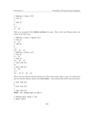
![Chapter 3 Principles of Programming Languages
#t
(pair? (car pair))
#f
(car (car pair))
car: expects argument of type pair; given 1
(procedure? pair?)
#t
Denotation of Pair values: The distinction between Pair typed Scheme expressions
(syntax), to their Pair values (semantics) must be made clear. (cons 1 2) is a Scheme
expression that evaluates into the Pair value (1 . 2). The Pair value cannot be evaluated
by the interpreter. Evaluation of (1 . 2) causes an error.
The value constructor, selectors and predicates of Pair are polymorphic procedures: They
can have multiple types, based on their argument types.
PAIR – the type constructor of type Pair: Pair is a composite polymorphic type. Its
type constructor is PAIR. It has 2 parameters:
PAIR(Number,Number) denotes the type (set) of all number pairs.
PAIR(Number,Procedure) denotes the type of all pairs of a number and a procedure.
PAIR(Number,T) is a polymorphic type expression, denoting all Pair types whose first
component is Number.
Infix notation: The Pair type constructor PAIR has also an infix notation, written
with the * symbol. For example, PAIR(Number,Number) is written Number*Number, and
PAIR(T1,T2) is written T1*T2. Indeed, in denoting the type of procedures we use the Pair
(and more generally Tuple) infix notation for the argument types. For example, the type of
+ is [Number*Number – Number]. In this expression, the Procedure type constructor –
takes 2 arguments: Number*Number, Number.
Values of the Pair type are usually denoted with infix notation. In Scheme, values
of (cons e1 e2) are denoted (printed) (value of e1 . value of e2); in ML, the
value constructor for pairs is written using infix notation: (e1 , e2).
Summary of the Pair type:
1. Type constructor: PAIR – a polymorphic type constructor, that takes 2 type ex-pressions
as arguments.
2. Value constructor: cons – Can take any values of a Scheme type.
cons: T1,T2 – PAIR(T1,T2)
Type of cons: [T1*T2 – PAIR(T1,T2)]
132](https://image.slidesharecdn.com/principlesofprogramminglanguages-140901163422-phpapp01/85/Principles-of-programming-languages-137-320.jpg)
![Chapter 3 Principles of Programming Languages
3. Selectors: car, cdr.
Type of car: [PAIR(T1,T2) – T1]
Type of cdr: [PAIR(T1,T2) – T2]
4. Predicates: pair?, equal?
Type of pair?: [T – Boolean]
Type of equal?: [T1*T2 – Boolean]
Recursively defined pairs: The Church numbers type is defined inductively as follows:
Zero is a Church number, and for a Church number c, S(c) is also a Church number. Church
numbers provide symbolic representation for the natural numbers, where the numbers
0, 1, 2, 3, ... are represented by the Church numbers Zero, S(Zero), S(S(Zero)),
S(S(S(Zero))), ... .
Church numbers can be represented (implemented) using pairs as follows: Zero, (S .
Zero), (S . (S . Zero)), (S . (S . (S . Zero))), ... . This representation is cre-ated
by the Scheme expressions: ’Zero, (cons ’S ’Zero), (cons ’S (cons ’S ’Zero)),
(cons ’S (cons ’S (cons ’S ’Zero))), ... . The following procedure creates the nth
Church number using this representation:
Signature: church(x)
Purpose: Computes the nth Church number.
type: Number - Symbol union PAIR(Symbol,PAIR)
(define church
(lambda (n)
(if (zero? n)
’Zero
(cons ’S (church (- n 1))))
))
(church 0)
Zero
(church 1)
(S . Zero)
(church 4)
(S S S S . Zero)
Note that the type of pairs returned by the procedure church cannot be expressed within the
limited type language we have introduced, since we have no means for defining recursive
types. Therefore, we use just the PAIR type constructor with no parameters.
More Pair procedures:
133](https://image.slidesharecdn.com/principlesofprogramminglanguages-140901163422-phpapp01/85/Principles-of-programming-languages-138-320.jpg)
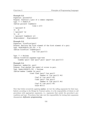
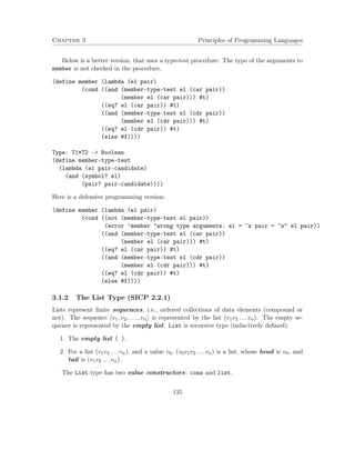
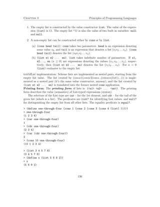
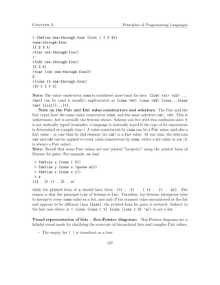
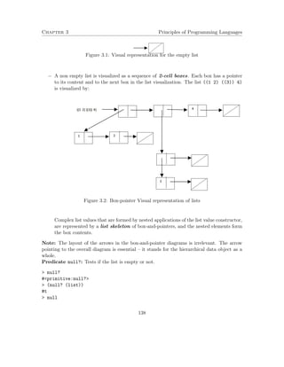
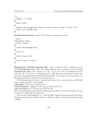
![Chapter 3 Principles of Programming Languages
Summary of the List type:
1. Type constructors: For homogeneous lists, LIST(T) – a polymorphic type construc-tor
that takes a single type expression as argument; for heterogeneous lists, LIST –
that takes no parameters.
2. Value constructors: cons, list.
Type of list: [T1*...*Tn – LIST], and also [T*...*T – LIST(T)], n 0.
Type of cons: [T*LIST – LIST], and also [T*LIST(T) – LIST(T)].
3. Selectors: car, cdr.
Type of car: [LIST – T] and also [LIST(T) – T].
Type of cdr: [LIST – LIST] and also [LIST(T) – LIST(T)].
Preconditions for (car list) and (cdr list): list != ().
4. Predicates: list?, null?, equal?
Type of list?: [T – Boolean]
Type of null?: [T – Boolean]
Type of equal?: [T1*T2 – Boolean]
3.1.2.1 Some useful List operations:
1. Composition of cons, car, cdr:
(define x (list 5 6 8 2))
x
(5 6 8 2)
(car x)
5
(cdr x)
(6 8 2)
(cadr x)
6
(cddr x)
(8 2)
(caddr x)
8
(cdddr x)
(2)
(cadddr x)
2
(cddddr x)
140](https://image.slidesharecdn.com/principlesofprogramminglanguages-140901163422-phpapp01/85/Principles-of-programming-languages-145-320.jpg)
![Chapter 3 Principles of Programming Languages
()
(cons 2 x)
(2 5 6 8 2)
(cons x x)
((5 6 8 2) 5 6 8 2)
Question: Consider the expressions (cons 1 2) and (list 1 2). Do they have the
same value?
2. Selector list-ref: Selects the nth element of a list. Its type is [LIST*Number –
T] or [LIST(T)*Number – T].
(define (list-ref items n)
(if (= n 0)
(car items)
(list-ref (cdr items) (- n 1))))
(define squares (list 1 4 9 16 25 36))
(list-ref 4 squares)
25
3. Operator length:
Reductional (recursive, inductive) definition:
The length of a list is the length of its tail (cdr) + 1.
The length of the empty list is 0.
(define (length items)
(if (null? items)
0
(+ 1 (length (cdr items)))))
WARNING: redefining built-in length
(length squares)
6
141](https://image.slidesharecdn.com/principlesofprogramminglanguages-140901163422-phpapp01/85/Principles-of-programming-languages-146-320.jpg)
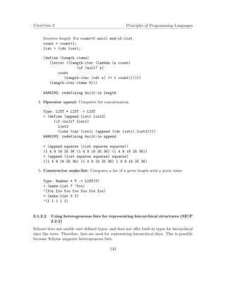
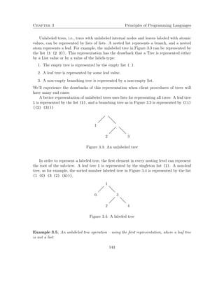
![Chapter 3 Principles of Programming Languages
Signature: count-leaves(x)
Purpose: Count the number of leaves in an unlabeled tree (a selector):
** The count-leaves of an empty tree is 0.
** The count-leaves of a leaf is 1.
A leaf is not represented by a list.
** The count-leaves of a non-empty and not leaf tree T is the count-leaves of
the first branch (car) + the count-leaves of all other branches (cdr).
Type: [LIST union Number union Symbol union Boolean - Number]
(define (count-leaves x)
(cond ((null? x) 0)
((not (list? x)) 1)
(else (+ (count-leaves (car x))
(count-leaves (cdr x))))))
(define x (cons (list 1 2) (list 3 4)))
x
((1 2) 3 4)
(length x)
3
(count-leaves x)
4
(list x x)
(((1 2) 3 4) ((1 2) 3 4))
(length (list x x))
2
(count-leaves (list x x))
8
3.1.3 Type Correctness with the Pair and List Types
Typing rules for pairs and lists:
The Pair and List operations are Scheme primitives (no special operators). Therefore, the
Primitive procedure typing axiom has to be extended for the new primitives.
Pairs:
For every type environment Tenv and type expressions S,S1,S2:
Tenv |- cons:[S1*S2 - PAIR(S1,S2)]
Tenv |- car:[PAIR(S1,S2) - S1]
Tenv |- cdr:[PAIR(S1,S2) - S2]
Tenv |- pair?:[S - Boolean]
144](https://image.slidesharecdn.com/principlesofprogramminglanguages-140901163422-phpapp01/85/Principles-of-programming-languages-149-320.jpg)
![Chapter 3 Principles of Programming Languages
Tenv |- equal?:[PAIR(S1,S2)*PAIR(S1,S2) - Boolean]
Homogeneous lists:
For every type environment Tenv and type expression S:
Tenv |- list:[Empty - LIST(S)]
Tenv |- list:[S* ...*S - LIST(S)] n 0
Tenv |- cons:[S*LIST(S) - LIST(S)]
Tenv |- car:[LIST(S) - S]
Tenv |- cdr:[LIST(S) - LIST(S)]
Tenv |- null?:[LIST(S) - Boolean]
Tenv |- list?:[S - Boolean]
Tenv |- equal?:[LIST(S)*LIST(S) - Boolean]
Heterogeneous lists:
For every type environment Tenv and type expression S:
Tenv |- list:[Empty - LIST]
Tenv |- cons:[S*LIST - LIST]
Tenv |- car:[LIST - S]
Tenv |- cdr:[LIST - LIST]
Tenv |- null?:[LIST - Boolean]
Tenv |- list?:[S - Boolean]
Tenv |- equal?:[LIST*LIST - Boolean]
Example 3.6. Derive the type of the firstFirst procedure. Its definition:
(define firstFirst (lambda(pair)
(car (car pair))))
We derive a type for the lambda form: Instantiation of the Variable axiom and the
Primitive procedure Pair axiom (an arbitrary decision, and with renaming):
1. {pair-T1 } |- pair:T1
2. { } |- car:[PAIR(T2,T3) - T2]
Typing (car pair) – Applying the Application typing rule to statements 1,2, with type
substitution {S1=T1=PAIR(T2,T3), S=T2}:
3. {pair- PAIR(T2,T3)} |- (car pair):T2
Typing (car (car pair)) – In order to apply the Application typing rule to statements
3,2, we first have to rename these statements:
145](https://image.slidesharecdn.com/principlesofprogramminglanguages-140901163422-phpapp01/85/Principles-of-programming-languages-150-320.jpg)
![Chapter 3 Principles of Programming Languages
2’. { } |- car:[PAIR(T21,T31) - T21]
3’. {pair- PAIR(T22,T32)} |- (car pair):T22
Applying the Application typing rule to statements 2’,3’, with type substitution
{S1=T22=PAIR(T21,T31), S=T21}:
4. {pair-PAIR(PAIR(T21,T31),T32 ) } |- (car (car pair)):T21
Application of typing rule Procedure to statement 4, with type substitution
{S1=PAIR(PAIR(T21,T31),T32), U1=T21}:
5. { } |- (lambda (pair) (car (car pair))):
[PAIR(PAIR(T21,T31),T32) - T21]
Following this definition, the type of firstFirst is {[PAIR(PAIR(T21,T31),T32) – T21]},
and well typed derivations can end with the type assignment
{firstFirst-PAIR(PAIR(T21,T31),T32) – T21}.
Example 3.7. Type derivation for (firstFirst (cons (cons 1 2) 3)):
Instantiation of the Number axiom, Variable axiom, and the Primitive procedure
Pair axiom (an arbitrary decision, and with renaming):
1. { } |- 1:Number
2. { } |- 2:Number
3. { } |- 3:Number
4. { } |- cons:[T1*T2 - PAIR(T1,T2)]
5. {firstFirst-T3} |- firstFirst:T3
Typing (cons 1 2) – Applying the Application typing rule to statements 1,2,4, with type
substitution {S1=Number, S2=Number, S=PAIR(Number,Number), T1=Number, T2=Number}:
6. { } |- (cons 1 2):PAIR(Number,Number)
Typing (cons (cons 1 2) 3) – Applying the Application typing rule to statements 6,3,4,
with type substitution {S1=PAIR(Number,Number), S2=Number,
S=PAIR(PAIR(Number,Number),Number), T1=PAIR(Number,Number), T2=Number}:
7. { } |- (cons (cons 1 2) 3):PAIR(PAIR(Number,Number),Number)
Typing (firstFirst (cons (cons 1 2) 3)) – Applying the Application typing rule to
statements 7,5, with type substitution {S1=PAIR(PAIR(Number,Number),Number), S=T4,
T3=[PAIR(PAIR(Number,Number),Number) – T4]}:
7. {firstFirst- [PAIR(PAIR(Number,Number),Number) - T4]} |-
(firstFirst (cons (cons 1 2) 3)):T4
146](https://image.slidesharecdn.com/principlesofprogramminglanguages-140901163422-phpapp01/85/Principles-of-programming-languages-151-320.jpg)
![Chapter 3 Principles of Programming Languages
The definition of firstFirst justifies derivations whose last typing statement has the type
assignment {firstFirst-PAIR(PAIR(T21,T31),T32) – T21}. The type assignment in
statement 7 is an instance of this type assignment, under the type substitution
{T21=T31=T32=Number}. Therefore, the type derivation of (firstFirst (cons (cons 1
2) 3)) is correct.
3.2 Data Abstraction: Abstract Data Types
Data abstraction intends to separate usage from implementation (also termed concrete
representation).
Client level – Usage: The parts of the program that use the data objects, i.e., the clients,
access the data objects via operations, such as set union, intersection, selection. They make
no assumption about how the data objects are implemented.
Supplier level – Implementation: The parts of the program that implement the data
objects provide procedures for selectors (getters in Object-Oriented programming) and
constructors. Constructors are the glue for constructing compound data objects, and
selectors are the means for splitting compound objects. The connection between the ab-stract
conceptual (client) level of usage to the concrete level of implementation is done by
implementing the client needs in terms of the constructors and selectors.
The principle of data abstraction is the separation between these levels:
2. Client Level
||
||
||/
/
1. Abstract Data Types (ADTs):
Data operators: Constructors, selectors, predicates
Correctness rules (Invariants)
/
/||
||
||
3. Supplier (implementation) Level
Rules of correctness (invariants): An implementation of data objects is verified (tested
to be true) by rules of correctness (invariants). An implementation that satisfies the cor-rectness
rules is correct. For example, every implementation of arrays that satisfies
get(A[i], set(A[i],val)) = val
for an array A, and reference index i, is correct. Correct implementations can still differ in
other criteria, like space and time efficiency.
147](https://image.slidesharecdn.com/principlesofprogramminglanguages-140901163422-phpapp01/85/Principles-of-programming-languages-152-320.jpg)
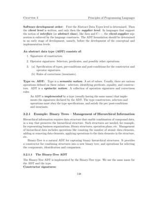
![Chapter 3 Principles of Programming Languages
Signature: make-binary-tree(l,r)
Purpose: Returns a binary tree whose left sub-tree is l
and whose right sub-tree is r
Type: [Binary-Tree*Binary-Tree - Binary-Tree]
Pre-condition: binary-tree?(l) and binary-tree?(r)
Signature: make-leaf(d)
Purpose: Returns a leaf binary-tree whose data element is d
Type: [T - Binary-Tree]
Selector signatures:
Signature: left-tree(r), right-tree(r)
Purpose: (left-tree t): Returns the left sub-tree of the binary-tree t.
(right-tree t): Returns the right sub-tree of the binary-tree t.
Type: [Binary-Tree - Binary-Tree]
Pre-condition: composite-binary-tree?(t)
Signature: leaf-data(r)
Purpose: Returns the data element of the leaf binary-tree t.
Type: [Binary-Tree - T]
Pre-condition: leaf?(t)
Predicate signatures:
Signature: leaf?(t)
Type: [T - Boolean]
Post-condition: true if t is a leaf -- constructed by make-leaf
Signature: composite-binary-tree?(t)
Type: [T - Boolean]
Post-condition: true if t is a composite binary-tree -- constructed by
make-binary-tree
Signature: binary-tree?(t)
Type: [T - Boolean]
Post-condition: result = (leaf?(t) or composite-binary-tree?(t) )
Signature: equal-binary-tree?(t1, t2)
Type: [Binary-Tree*Binary-Tree - Boolean]
Invariants:
149](https://image.slidesharecdn.com/principlesofprogramminglanguages-140901163422-phpapp01/85/Principles-of-programming-languages-154-320.jpg)
![Chapter 3 Principles of Programming Languages
leaf-data(make-leaf(d)) = d
left-tree(make-binary-tree(l,r)) = l
right-tree(make-binary-tree(l,r)) = r
leaf?(make-leaf(d)) = true
leaf?(make-binary-tree(l,r)) = false
composite-binary-tree?(make-binary-tree(l,r)) = true
composite-binary-tree?(make-leaf(d)) = false
Note that the Binary-Tree operations have the Binary-Tree as their type. That is, the
ADT defines a new type, that extends the type language. In practice, Scheme does not
recognize any of the ADTs that we define. This is a programmers’ means for achieving
software abstraction. Therefore, our typing rule is:
1. ADT operations are declared as introducing new types.
2. Clients of the ADT are expressed (typed) using the new ADT types.
3. Implementers (suppliers) of an ADT use already implemented types or ADTs types.
3.2.1.2 Client level: Binary-Tree management
Some client operations may be:
;Signature: count-leaves(tree)
;Purpose: Count the number of leaves of ’tree’
;Type: [binary-Tree - number]
(define count-leaves
(lambda (tree)
(if (composite-binary-tree? tree)
(+ (count-leaves (left-tree tree))
(count-leaves (right-tree tree)))
1)))
;Signature: has-leaf?(item,tree)
;Purpose: Does ’tree’ includes a leaf labaled ’item’
;Type: [T*Binary-Tree - Boolean]
(define has-leaf?
(lambda (item tree)
(if (composite-binary-tree? tree)
(or (has-leaf? item (left-tree tree))
(has-leaf? item (right-tree tree)))
(equal? item (leaf-data tree)))))
150](https://image.slidesharecdn.com/principlesofprogramminglanguages-140901163422-phpapp01/85/Principles-of-programming-languages-155-320.jpg)
![Chapter 3 Principles of Programming Languages
;Signature: add-leftmost-leaf(item,tree)
;Purpose: Creates a binary-tree with ’item’ added as a leftmost leaf to ’tree’
;Type: [T*Binary-Tree - Binary-Tree]
(define add-leftmost-leaf
(lambda (item tree)
(if (composite-binary-tree? tree)
(make-binary-tree (add-leftmost-leaf item (left-tree tree))
(right-tree tree))
(make-binary-tree (make-leaf item)
tree))
))
Note: The client operations are written in a non-defensive style. That is, correct type
of arguments is not checked. They should be associated with appropriate type-checking
procedures, that their clients should apply prior to their calls, or be extended with defensive
correct application tests.
3.2.1.3 Supplier (implementation) level
In this level we define the Binary-Tree type that implements the Binary-Tree ADT. The
implementation is in terms of the already implemented List (not necessarily homogeneous)
type. We use the first representation discussed in subsection 3.1.2.2, where the unlabeled
binary-tree in Figure 3.3, is represented by the list (1 (2 3)). In every implementation,
the Binary-Tree type is replaced by an already known type. We present two type implemen-tations.
Binary-Tree implementation I: A binary-tree is represented as a heterogeneous list.
;Signature: make-binary-tree(l,r)
;Type: [(LIST union T1)*(LIST union T2) - LIST]
;Pre-condition: binary-tree?(l) and binary-tree?(r)
(define make-binary-tree
(lambda (l r)
(list l r)))
;Signature: make-leaf(d)
;Type: [T - T]
(define make-leaf
(lambda (d) d))
;Signature: left-tree(t)
;Type: [LIST - LIST union T]
151](https://image.slidesharecdn.com/principlesofprogramminglanguages-140901163422-phpapp01/85/Principles-of-programming-languages-156-320.jpg)
![Chapter 3 Principles of Programming Languages
;Pre-condition: composite-binary-tree?(t)
(define left-tree
(lambda (t) (car t)))
;Signature: right-tree(t)
;Type: [LIST - LIST union T]
;Pre-condition: composite-binary-tree?(t)
(define right-tree
(lambda (t) (cadr t)))
;Signarture: leaf-data(t)
;Type: [T - T]
;Pre-condition: leaf?(t)
(define leaf-data
(lambda (t) t))
;Signarture: leaf?(t)
;Type: [T - Boolean]
(define leaf?
(lambda (t) #t))
;Signarture: composite-binary-tree?(t)
;Type: [T - Boolean]
(define composite-binary-tree?
(lambda (t)
(and (list? t)
(list? (cdr t))
(null? (cddr t))
(binary-tree? (left-tree t))
(binary-tree? (right-tree t)))
))
;Signarture: binary-tree?(t)
;Type: [T - Boolean]
(define binary-tree?
(lambda (t) (or (leaf? t) (composite-binary-tree? t))))
;Signature: equal-binary-tree?(t1,t2)
;Type: [(LIST union T1)*(LIST union T2) - Boolean]
;Pre-condition: binary-tree?(t1) and binary-tree?(t2)
(define equal-binary-tree?
152](https://image.slidesharecdn.com/principlesofprogramminglanguages-140901163422-phpapp01/85/Principles-of-programming-languages-157-320.jpg)
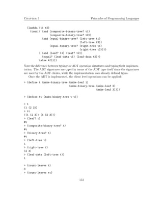
![Chapter 3 Principles of Programming Languages
6
(has-leaf? 2 t)
#t
(add-leftmost-leaf 0 t)
((0 1) (2 3))
Does the implementation satisfy the invariants of the Binary-Tree ADT? The
invariants are:
leaf-data(make-leaf(d)) = d
left-tree(make-binary-tree(l,r)) = l
right-tree(make-binary-tree(l,r)) = r
leaf?(make-leaf(d)) = true
leaf?(make-binary-tree(l,r)) = false
composite-binary-tree?(make-binary-tree(l,r)) = true
composite-binary-tree?(make-leaf(d)) = false
The first three invariants are satisfied. But what about the last one? Consider, for example:
(composite-binary-tree? (make-leaf (list 5 6)))
#t
(leaf? (make-leaf (list 5 6)))
#t
(has-leaf? (list 5 6) (make-leaf (list 5 6)))
#f
What is the problem? There is no way to distinguish leaves that carry data of 2-element
lists from composite-binary trees. The leaf predicate just accepts any argument, and the
composite-binary-tree? tests whether its argument is a 2 element list of data of the
binary-tree structure.
The Binary-Tree implementation does not provide means for singling out binary-trees
from lists of an appropriate structure, and in particular, cannot distinguish leaves that carry
list data from composite-binary-trees. The solution is to tag the implementation values by
their intended type.
Tagged-data ADT: The idea is to introduce an interface of operations that enable iden-tification
of data. The identification means can be any kind of tagging. The interface
below assumes that tags are symbols. The Tagged-data ADT defines a polymorphic type:
Tagged-data(T):
Signature: attach-tag(x,tag)
Purpose: Construct a tagged-data value
Type: [T*Symbol - Tagged-data(T)]
154](https://image.slidesharecdn.com/principlesofprogramminglanguages-140901163422-phpapp01/85/Principles-of-programming-languages-159-320.jpg)
![Chapter 3 Principles of Programming Languages
Signature: get-tag(tagged)
Purpose: Select the tag from a tagged-data value
Type: [Tagged-data(T) - Symbol]
Signature: get-content(tagged)
Purpose: Select the data from a tagged-data value
Type: [Tagged-data(T) - T]
Signature: tagged-data?(datum)
Purpose: Identify tagged-data values
Type: [T - Boolean]
Signature: tagged-by?(tagged,tag)
Purpose: Identify tagged-data values
Type: [T*Symbol - Boolean]
Invariants:
get-tag(attach-tag(x.tag)) = tag
get-content(attach-tag(x,tag)) = x
tagged-data?(d) = exist x and tag such that d=attach-tag(x,tag)
tagged-by?(tag’,attach-tag(x,tag)) = (tag’ = tag)
Binary-tree implementation II – Tagged-data based implementation using het-erogeneous
lists:
;Signature: make-binary-tree(l,r)
;Type: [(LIST union T1)*(LIST union T2) - Tagged-data(LIST)]
;Pre-condition: binary-tree?(l) and binary-tree?(r)
(define make-binary-tree
(lambda (l r)
(attach-tag (list l r) ’composite-binary-tree)))
;Signature: make-leaf(d)
;Type: [T - Tagged-data(T)]
(define make-leaf
(lambda (d)
(attach-tag d ’leaf)))
;Signature: left-tree(t)
;Type: [Tagged-data(LIST) - Tagged-data(LIST union T)]
155](https://image.slidesharecdn.com/principlesofprogramminglanguages-140901163422-phpapp01/85/Principles-of-programming-languages-160-320.jpg)
![Chapter 3 Principles of Programming Languages
;Pre-condition: composite-binary-tree?(t)
(define left-tree
(lambda (t) (car (get-content t))))
;Signature: right-tree(t)
;Type: [Tagged-data(LIST) - Tagged-data(LIST union T)]
;Pre-condition: composite-binary-tree?(t)
(define right-tree
(lambda (t) (cadr (get-content t))))
;Signarture: leaf-data)t)
;Type: [Tagged-data(T) - T]
;Pre-condition: leaf?(t)
(define leaf-data
(lambda (t) (get-content t)))
;Type: [T - Boolean]
(define leaf?
(lambda (t) (tagged-by? t ’leaf)))
;Type: [T - Boolean]
(define composite-binary-tree?
(lambda (t)
(tagged-by? t ’composite-binary-tree)))
binary-tree? and equal-binary-tree? are not modified, as they are implemented in
terms of other Binary-Tree ADT operations. Client operations stay intact.
Implementation for the Tagged-data ADT: In order to apply the Tagged-data based
implementation of Binary-tree we still need an implementation for the Tagged-data ADT.
Here is one possibility – Pair based:
;Signature: attach-tag(x,tag)
;Type: [Symbol*T - PAIR(Symbol, T)]
(define attach-tag (lambda (x tag) (cons tag x)))
;Signature: get-tag(tagged)
;Type: PAIR(Symbol,T) - Symbol
(define get-tag (lambda (tagged) (car tagged)))
;Signature: get-content(tagged)
;Type: [PAIR(Symbol,T) - T]
156](https://image.slidesharecdn.com/principlesofprogramminglanguages-140901163422-phpapp01/85/Principles-of-programming-languages-161-320.jpg)
![Chapter 3 Principles of Programming Languages
(define get-content (lambda (tagged) (cdr tagged)))
;Signature: tagged-data?(datum)
;Type: [T - Boolean]
(define tagged-data?
(lambda (datum)
(and (pair? datum) (symbol? (car datum))) ))
;Signature: tagged-by?(tagged,tag)
;Type: [T*Symbol - Boolean]
(define tagged-by?
(lambda (tagged tag)
(and (tagged-data? tagged)
(eq? (get-tag tagged) tag))))
(define tagged-1 (attach-tag 1 ’number))
(get-tag tagged-1)
number
(get-content tagged-1)
1
(tagged-data? tagged-1)
#t
Once the Tagged-data ADT is implemented, its clients – Binary-Tree, and the clients of
the clients can be applied:
(define t (make-binary-tree (make-leaf 1)
(make-binary-tree (make-leaf 2)
(make-leaf 3))))
(define tt (make-binary-tree t t))
t
(composite-binary-tree (leaf . 1) (composite-binary-tree (leaf . 2) (leaf . 3)))
tt
(composite-binary-tree
(composite-binary-tree (leaf . 1) (composite-binary-tree (leaf . 2) (leaf . 3)))
(composite-binary-tree (leaf . 1) (composite-binary-tree (leaf . 2) (leaf . 3))))
(leaf? t)
#f
(composite-binary-tree? t)
#t
157](https://image.slidesharecdn.com/principlesofprogramminglanguages-140901163422-phpapp01/85/Principles-of-programming-languages-162-320.jpg)
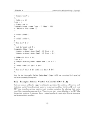
![Chapter 3 Principles of Programming Languages
3.2.2.1 The Rat ADT
The Rat ADT would be implemented by the Rat type. We use the same name for the ADT
and the type.
Constructor signature:
Signature: make-rat(n,d)
Purpose: Returns a rational number whose numerator is the
integer n, and whose denominator is the integer d
Type: [Number*Number - Rat]
Pre-condition: d != 0, n and d are integers.
Selector signatures:
Signature: numer(r), denom(r)
Purpose: (numer r): Returns the numerator of the rational number r.
(denom r): Returns the denominator of the rational number r.
Type: [Rat - Number]
Post-condition for denom: result != 0.
Predicate signatures:
Signature: rat?(r)
Type: [T - Boolean]
Post-condition: result = (Type-of(r) = Rat)
Signature: equal-rat?(x, y)
Type: [Rat*Rat - Boolean]
The ADT invariants will be discussed following the presentation of several alternative im-plementations.
Note that the Rat operations are declared as have the Rat type. That is, we use the ADT
as a new type, that extends the type language. In practice, Scheme does not recognize any of
the ADTs that we define. This is a programmers means for achieving software abstraction.
Therefore, our typing rule is:
1. ADT operations are declared as introducing new types.
2. Clients of the ADT are expressed (typed) using the new ADT types.
3. Implementers (suppliers) of an ADT use already implemented types or ADTs.
159](https://image.slidesharecdn.com/principlesofprogramminglanguages-140901163422-phpapp01/85/Principles-of-programming-languages-164-320.jpg)
![Chapter 3 Principles of Programming Languages
3.2.2.2 Client level: Rational-number arithmetic
The client operations for using rationals are: Addition, subtraction, multiplication,
division, and equality. In addition, the client level includes a print-rat operation, for
nice intuitive display of rationals. All operations are implemented in terms of the Rat ADT:
Type: [Rat*Rat - Rat] for add-rat, sub-rat, mul-rat, div-rat.
(define add-rat
(lambda (x y)
(make-rat (+ (* (numer x) (denom y))
(* (denom x) (numer y)))
(* (denom x) (denom y)))))
(define sub-rat
(lambda (x y)
(make-rat (- (* (numer x) (denom y))
(* (denom x) (numer y)))
(* (denom x) (denom y)))))
(define mul-rat
(lambda (x y)
(make-rat (* (numer x) (numer y))
(* (denom x) (denom y)))))
(define div-rat
(lambda (x y)
(make-rat (* (numer x) (denom y))
(* (denom x) (numer y)))))
Type: Rat - Void
(define print-rat
(lambda (x)
(display (numer x))
(display /)
(display (denom x))
(newline)))
Note: In all Rat arithmetic procedures, clients should verify that the arguments are of
type Rat (using the rat? procedure).
160](https://image.slidesharecdn.com/principlesofprogramminglanguages-140901163422-phpapp01/85/Principles-of-programming-languages-165-320.jpg)
![Chapter 3 Principles of Programming Languages
3.2.2.3 Supplier (implementation) level
In this level we define the Rat type that implements the Rat ADT. The implementation is
in terms of the already implemented Pair type. The implementation depends on a repre-sentation
decision: What are the values of the Rat type. In every implementation, the Rat
type is replaced by an already known type.
We present several Rat type implementations. All are based on the Pair type, but differ
in the actual integers from which the values of Rat are constructed.
Rat implementation I – Based on an unreduced Pair representation: A rational
number is represented by a pair of its numerator and denominator. That is, Rat=PAIR(Number,Number):
Signature: make-rat(n,d)
Type: [Number *Number - PAIR(Number,Number)]
Pre-condition: d != 0
(define make-rat (lambda (n d) (cons n d)))
Type: [PAIR(Number,Number) - Number]
(define numer (lambda (r) (car r)))
Type: [PAIR(Number,Number) - Number]
(define denom (lambda(r) (cdr r)))
Type: [T -- boolean]
(define rat? (lambda (r) (pair? r)))
Type: [PAIR(Number,Number)*PAIR(Number,Number) - Number]
(define equal-rat?
(lambda (x y)
(= (* (numer x) (denom y))
(* (numer y) (denom x))))
Pre-condition and argument types tests:
(define make-rat-pre-condition-argument-type-test
(lambda (n d)
(and (integer? n) (integer? d) (not (= d 0)))))
(define numer-argument-type-test
(lambda (r)
(rat? r))
161](https://image.slidesharecdn.com/principlesofprogramminglanguages-140901163422-phpapp01/85/Principles-of-programming-languages-166-320.jpg)
![Chapter 3 Principles of Programming Languages
(define denom-argument-type-test
(lambda (r)
(rat? r)))
Once the ADT is implemented, the client level operations can be applied:
(define one-half (make-rat 1 2))
(define two-sixth (make-rat 2 6))
(print-rat (add-rat one-half two-sixth))
10/12
(print-rat (mul-rat one-half two-sixth))
2/12
(print-rat (div-rat two-sixth one-half))
4/6
(div-rat two-sixth one-half)
(4 . 6)
(define x (print-rat (div-rat two-sixth one-half)))
x
???????
Note on the types of the implemented Rat operations: Note the difference be-tween
typing the ADT operation signatures and typing their implementation. The ADT
signatures are typed in terms of the ADT itself since the signatures are used by the ADT
clients, while the implementation uses already defined ADTs. For the above implementa-tion
Rat=PAIR(Number,Number), the Rat type in the ADT declaration is replaced by the
implementation type PAIR(Number,Number). For example, in the ADT declaration the type
of make-rat is [Number*Number – Rat], while the type of the implemented make-rat is
[Number*Number – PAIR(Number,Number)].
Variation on the Rat operator definition: The Rat value constructor and selectors can
be defined as new names for the Scheme primitive Pair constructor and selectors:
(define make-rat cons)
(define numer car)
(define denom cdr)
(define rat? pair?)
make-rat
#primitive:cons
In the original definition, make-rat uses cons, and therefore is a compound procedure. In
the second definition, make-rat is another name for the primitive procedure which is the
value of cons. In this case there is a single procedure with two names. The second option
is more efficient in terms of time and space.
162](https://image.slidesharecdn.com/principlesofprogramminglanguages-140901163422-phpapp01/85/Principles-of-programming-languages-167-320.jpg)
![Chapter 3 Principles of Programming Languages
Rat implementation II – Tagged unreduced Pair representation: The intention
behind the previous implementation of Rat is to identify the Rat type with the type
PAIR(Number,Number). But the identifying predicate rat? is defined by:
(define rat? (lambda (r) (pair? r))).
Therefore, rat? identifies any pair as a rational number implementation, including for
example, the pairs (a . b), and (1 . 0):
(rat? (make-rat 3 2))
#t
(rat? (cons (quote a) (quote b)))
#t
The problem is that the Rat implementation does not provide any means for singling out
pairs that implement Rat values from all other pairs. The solution is to tag the implemen-tation
values by their intended type.
Tagged Pair based implementation: The tagged implementation is
Rat=Tagged-data(PAIR(Number,Number))=PAIR(Symbol,PAIR(Number,Number)). equal-rat?
is not listed as it does not change.
Signature: make-rat(n, d)
Type: [Number*Number - Tagged-data(PAIR(Number,Number))]
Pre-condition: d != 0; n and d are integers.
(define make-rat
(lambda (n d)
(attach-tag (cons n d) ’rat)))
Signature: numer(r)
Type: [Tagged-data(PAIR(Number,Number)) - Number]
(define numer
(lambda (r)
(car (get-content r))))
Signature: denom(r)
Type: [Tagged-data(PAIR(Number,Number)) - Number]
Post-condition: result != 0
(define denom
(lambda (r)
(cdr (get-content r))))
Signature: rat?(r)
Type: [T - Boolean]
163](https://image.slidesharecdn.com/principlesofprogramminglanguages-140901163422-phpapp01/85/Principles-of-programming-languages-168-320.jpg)
![Chapter 3 Principles of Programming Languages
Post-condition: result = (Type-of(r) = Rat)
(define rat? (lambda (x) (tagged-by? x ’rat)))
(define one-half (make-rat 1 2))
(define two-sixth (make-rat 2 6))
(print-rat (add-rat one-half two-sixth))
10/12
(print-rat (mul-rat one-half two-sixth))
2/12
(define x (print-rat (div-rat two-sixth one-half)))
one-half
(rat 1 . 2)
(get-tag one-half)
rat
(content one-half)
(1 . 2)
(rat? one-half)
#t
(rat? (content one-half))
#f
(rat? (div-rat one-half two-sixth))
#t
Rat implementation III – Tagged, reduced at construction time Pair represen-tation:
The idea behind this implementation is to represent the rational number by a
reduced pair of numerator and denominator. The reduction uses the gcd procedure from
http://mitpress.mit.edu/sicp/code/ch2support.scm).
(define gcd
(lambda (a b)
(if (= b 0)
a
(gcd b (remainder a b)))))
The implementation is still: Rat=PAIR(Symbol,PAIR(Number,Number)). rat?, equal-rat?
are not listed as there is no change.
Signature: make-rat(n,d)
Type: [Number*Number - Tagged-data(PAIR(Number,Number))]
Pre-condition: d != 0; n and d are integers
(define make-rat
(lambda (n d)
164](https://image.slidesharecdn.com/principlesofprogramminglanguages-140901163422-phpapp01/85/Principles-of-programming-languages-169-320.jpg)
![Chapter 3 Principles of Programming Languages
(let ((g (gcd n d)))
(attach-tag (cons (/ n g) (/ d g)) ’rat))))
Signature: numer(r)
Type: [Tagged-data(PAIR(Number,Number)) - Number]
(define numer (lambda (r) (car (get-content r))))
Signature: denom(r)
Type: [Tagged-data(PAIR(Number,Number)) - Number]
Post-condition: result != 0
(define denom (lambda (r) (cdr (get-content r))))
(print-rat (div-rat two-sixth one-half))
2/3
(define one-half (make-rat 5 10))
one-half
(rat 1 . 2)
Rat implementation IV: Tagged, reduced at selection time Pair representation:
The idea behind this implementation is to represent the rational number by the given nu-merator
and denominator, but reduce them when queried. The implementation is still:
Rat=PAIR(Symbol,PAIR(Number,Number)). rat?, equal-rat? are not listed as there is no
change.
Signature: make-rat(n,d)
Type: [Number*Number - Tagged-data(PAIR(Number,Number))]
Pre-condition: d != 0 ; n and d are integers
(define make-rat
(lambda (n d)
(attach-tag (cons n d) ’rat)))
Signature: numer(r)
Type: [Tagged-data(PAIR(Number,Number)) - Number]
(define numer
(lambda (r)
(let ((g (gcd (car (get-content r))
(cdr (get-content r)))))
(/ (car (get-content r)) g))))
Signature: denom(r)
165](https://image.slidesharecdn.com/principlesofprogramminglanguages-140901163422-phpapp01/85/Principles-of-programming-languages-170-320.jpg)
![Chapter 3 Principles of Programming Languages
Type: [Tagged-data(PAIR(Number,Number)) - Number]
Post-condition: result != 0
(define denom
(lambda (r)
(let ((g (gcd (car (get-content r))
(cdr (get-content r)))))
(/ (cdr (get-content r)) g))))
Invariants of the Rat ADT: We get back now to the Rat ADT invariants. The role of
the invariants is to characterize correct implementations. Our intuition is that all presented
implementations are correct. Hence, we need rules that are satisfied by all implementations
above.
First suggestion:
numer(make-rat(n,d)) = n
denom(make-rat(n,d)) = d
Are these rules satisfied by all implementations above? The answer is no!. Implementations
III and IV do not satisfy them. Yet, our intuition is that these implementations are correct.
That means that the suggested invariants are too strict, and therefore reject acceptable
implementations.
Second suggestion:
numer(make-rat(n,d))/denom(make-rat(n,d)) = n/d
This invariant is satisfied by all of the above implementations.
Summary of the operations of the Rat ADT:
Signature: make-rat(n,d)
Purpose: Returns a rational number whose numerator is the
integer n, and whose denominator is the integer d
Type: [Number*Number - Rat]
Pre-condition: d != 0, n and d are integers.
Selector signatures:
Signature: numer(r), denom(r)
Purpose: (numer r): Returns the numerator of the rational number r.
(denom r): Returns the denominator of the rational number r.
Type: [Rat - Number]
Post-condition for denom: result != 0.
Predicate signatures:
166](https://image.slidesharecdn.com/principlesofprogramminglanguages-140901163422-phpapp01/85/Principles-of-programming-languages-171-320.jpg)
![Chapter 3 Principles of Programming Languages
Signature: rat?(r)
Type: [T - Boolean]
Post-condition: result = (Type-of(r) = Rat)
Signature: equal-rat?(x, y)
Type: [Rat*Rat - Boolean]
Rule of correctness (invariant):
[ (numer (make-rat n d)) / (denom (make-rat n d)) ] = n/d
3.2.3 What is Meant by Data? (SICP 2.1.3)
The question that motivates this subsection is: What is data? The notion of data is
usually understood as something consumed by procedures. But in functional languages,
procedures are first class citizens, i.e., handled like values of other types. Therefore in such
languages the distinction between data and procedures is especially obscure.
In order to clarify this issue we ask whether procedures can be used as data, i.e., con-sumed
by procedures. Specifically, we consider the previous Binary-Tree management or the
Rational Number arithmetic problem, where the implementations use the built-in Pair and
List types. We pose the problem:
Suppose that the Scheme application does not include built-in Pair or List types.
How can we build an implementation for the Binary-Tree and the Rat ADTs?
We solve the problem by:
1. Defining a Pair ADT: PAIR(T1,T2).
2. Defining a Pair type that implements the Pair ADT in terms of the Procedure type.
That is: PAIR(T1,T2) = [Symbol – (T1 union T2)].
The Pair ADT:
Signature: cons(x,y)
Type: [T1*T2 - PAIR(T1,T2)]
Signature: car(p)
Type: [PAIR(T1,T2) - T1]
Signature: cdr(p)
Type: [PAIR(T1,T2) - T2]
Signature: pair?(p)
167](https://image.slidesharecdn.com/principlesofprogramminglanguages-140901163422-phpapp01/85/Principles-of-programming-languages-172-320.jpg)
![Chapter 3 Principles of Programming Languages
Type: [T - Boolean]
Signature: equal-pair?(p1,p2)
Type: [PAIR(T1,T2)*PAIR(T1,T2) - Boolean]
Invariants:
(car (cons x y)) = x
(cdr (cons x y)) = y
Below are two implementations of the Pair ADT in terms of procedures. A pair is repre-sented
by a procedure, that enables selection of the pair components. The implementations
differ in their processing of the pair components. The first implementation, termed eager,
represents a pair as a procedure built specifically for selection of the pair components. The
second implementation, termed lazy, represents a pair as a procedure built for answering
any request about the pair components.
3.2.3.1 Pair implementation I: Eager Procedural representation
Signature: cons(x,y)
Type: [T1*T2 - [Symbol - (T1 union T2)]
(define cons
(lambda (x y)
(lambda (m)
(cond ((eq? m ’car) x)
((eq? m ’cdr) y)
(else (error Argument not ’car or ’cdr -- CONS m) ))) ))
Signature: car(pair)
Type: [[Symbol - (T1 union T2)] - T1]
(define car (lambda (pair) (pair ’car)))
Signature: cdr(pair)
Type: [[Symbol - (T1 union T2)] - T2]
(define cdr (lambda (pair) (pair ’cdr)))
Signature: equal-pair?(p1,p2)
Type: [[[(T1 union T2)] - T2]*[[(T1 union T2)] - T2] - Boolean]
(define equal-pair?
(lambda (p1 p2)
(and (equal? (car pair1) (car pair2))
(equal? (cdr pair1) (cdr pair2)) )))
168](https://image.slidesharecdn.com/principlesofprogramminglanguages-140901163422-phpapp01/85/Principles-of-programming-languages-173-320.jpg)
![Chapter 3 Principles of Programming Languages
A pair data value is a procedure, that stores the information about the pair components.
car takes a pair data value – a procedure – as an argument, and applies it to the symbol
car. cdr is similar, but applies its argument pair procedure to the symbol textttcdr. The
pair procedure, when applied to the symbol car, returns the value of the first parameter of
cons. Hence, (car (cons x y)), evaluates to the first pair component. The rule for cdr
holds for similar arguments. Note that the definition of cons returns a closure as its value,
but does not apply it!
applicative-eval[ (cons 1 2) ] ==*
closure (m)
(cond ((eq? m ’car) 1)
((eq? m ’cdr) 2)
(else (error Argument not ’car or ’cdr -- CONS m) ))
applicative-eval[ (car (cons 1 2 )) ] ==
applicative-eval[ car ] == closure (pair) (pair ’car)
applicative-eval[ (cons 1 2) ] ==* the cons closure as above
sub[pair, cons closure, (pair ’car) ] == (cons closure ’car)
reduce:
( (lambda (m)
(cond ((eq? m ’car) 1)
((eq? m ’cdr) 2)
(else (error Argument not ’car or ’cdr -- CONS m) )))
’car) ==*
applicative-eval, sub, reduce:
(cond ((eq? ’car ’car) 1)
((eq? ’car ’cdr) 2)
(else (error Argument not ’car or ’cdr -- CONS ’car) )) ==
1
(define x (cons 1 2))
x
#Closure (m) (cond ((eq? m ’car) x) ((eq? m ’cdr) y) (else (error
#Argument not ... ))))
(define y (car x))
y
1
(define z (cdr x))
z
2
(define w (cons y z))
169](https://image.slidesharecdn.com/principlesofprogramminglanguages-140901163422-phpapp01/85/Principles-of-programming-languages-174-320.jpg)
![Chapter 3 Principles of Programming Languages
(car w)
1
(cdr w)
2
cons
#Closure (x y) (lambda (m) (cond ((eq? m ’car) x) ((eq? m ’cdr) y)
(else (error ... ))))
car
#Closure (pair) (pair ’car)
Notes:
1. Pairs are represented as procedures that receive messages. A pair is created by ap-plication
of the cons procedure, that generates a new procedure for the defined pair.
Therefore, the variables x, w above denote different pair objects – different procedures
(recall that the Procedure type does not have an equality predicate).
2. The equal-pair? implementation uses the built-in primitive predicate equal?. Since
Pair is a polymorphic ADT, its implementation requires a polymorphic equality pred-icate,
that can be either built-in or written (for example, as a very long conditional of
value comparisons).
3. The technique of EAGER procedural abstraction, where data values are implemented
as procedures that take a message as input, is called message passing.
An alternative writing of this implementation, using a locally created procedure named
dispatch:
Signature: cons(x,y)
Type: [T1*T2 - [Symbol - T1 union T2 union String]
(define cons
(lambda (x y)
(letrec
((dispatch (lambda(m)
(cond ((eq: m ’car) x)
((eq? m ’cdr) y)
(else
(error Argument not ’car or ’cdr -- CONS m))))
))
dispatch)))
The Pair implementation does not support the predicate pair?. In order to implement
pair? we need an explicit typing, that should be planed as part of an overall types imple-mentation.
170](https://image.slidesharecdn.com/principlesofprogramminglanguages-140901163422-phpapp01/85/Principles-of-programming-languages-175-320.jpg)
![Chapter 3 Principles of Programming Languages
3.2.3.2 Pair implementation II: Lazy Procedural representation
The eager procedural implementation for the Pair ADT represents a Pair value as a proce-dure
that already prepared the computations for all known selectors. The lazy procedural
implementation defers everything: A Pair value is represented as a procedure that “‘waits”
for just any selector. In selection time, the given selector procedure is applied by the pair
components. The constructor does not prepare anything – it is truly lazy!
Signature: cons(x,y)
Type: [T1*T2 - [ [T1*T2 - T3] - T3]]
(define cons
(lambda (x y)
(lambda (sel) (sel x y))))
Signature: car(pair)
Type: [[ [T1*T2 - T3] - T3] - T1]
(define car
(lambda (pair)
(pair (lambda (x y) x))))
Signature: cdr(pair)
Type: [[ [T1*T2 - T3] - T3] - T2]
(define cdr
(lambda (pair)
(pair (lambda (x y) y))))
Evaluation examples:
applicative-eval[ (cons 1 2) ] ==
closure (sel) (sel 1 2)
applicative-eval[ (car (cons 1 2 )) ] ==*
applicative-eval[ car ] == closure (pair) (pair (lambda(x y) x))
applicative-eval[ (cons 1 2) ] ==* closure (sel) (sel 1 2)
sub, reduce:
applicative-eval[
( closure (sel) (sel 1 2) (lambda(x y) x) ) ] ==*
applicative-eval[ ( (lambda(x y) x) 1 2) ] ==
applicative-eval, sub, reduce:
1
Question: Assume that the Pair ADT has an additional operation function-value speci-fied
by the following contract:
171](https://image.slidesharecdn.com/principlesofprogramminglanguages-140901163422-phpapp01/85/Principles-of-programming-languages-176-320.jpg)
![Chapter 3 Principles of Programming Languages
Signature: sum-values(pair,f)
Purpose: Returns the sum of f values on the components of a pair of numbers
Type: [PAIR(Number,Number)*[Number - Number] - Number]
Example: sum-values((2 . 3),(lambda (x) (- x))) = -5
Add this operation to the eager and lazy procedural implementations of the ADT Pair.
Side comment: The lazy procedural implementation implements the Visitor
design pattern
Software design patterns [4] (http://www.cs.up.ac.za/cs/aboake/sws780/references/
patternstoarchitecture/Gamma-DesignPatternsIntro.pdf) is an approach that provides
solutions for typical problems that accrue in multiple contexts. Visitor is a well known
design pattern, suggested in [4]. Here is a short description taken from wikipedia:
In object-oriented programming and software engineering, the visitor de-sign
pattern is a way of separating an algorithm from an object structure
it operates on. A practical result of this separation is the ability to add new
operations to existing object structures without modifying those structures.
In essence, the visitor allows one to add new virtual functions to a family of
classes without modifying the classes themselves; instead, one creates a visitor
class that implements all of the appropriate specializations of the virtual func-tion.
The visitor takes the instance reference as input, and implements the goal
through double dispatch.
In the Visitor design pattern, a client holds an operation – the visitor, and an element
– the object, where the exact identity of both is not known to the client. The client lets
the visitor approach the object (by applying the accept method of the object. The object
then dispatches itself to the visitor. After this double dispatch – visitor to object and object
to visitor, the concrete visitor holds the concrete object and can apply its operation on the
object.
The lazy procedural implementation is based on a similar double dispatch: In order to
operate, a selector gives itself (visits) to an object, and then the object dispatches itself to
the operator for applying its operation.
3.2.3.3 Comparison of the eager and the lazy procedural implementations:
1. Eager: More work at constructions time. Immediate at selection time.
Lazy: Immediate at construction time. More work at selection time.
2. Eager: Selectors that are not simple getters can have any arity.
Lazy: selectors can be added freely, but must have the same arity.
172](https://image.slidesharecdn.com/principlesofprogramminglanguages-140901163422-phpapp01/85/Principles-of-programming-languages-177-320.jpg)
![Chapter 3 Principles of Programming Languages
3.2.4 The Sequence Interface (includes examples from SICP 2.2.3)
Object-oriented programming languages support a variety of interfaces and implementation
utilities for aggregates, like Set, List, Array. These interfaces declare standard collection
services like has-next(), next(), item-at(ref), size(), is-empty() and more.
Functional languages provide furthermore, powerful sequence operations that put an
abstraction barrier (ADT interface) between clients running sequence applications to
the sequence implementation. The advantage is the separation between usage and implemen-tation:
Ability to develop abstract level client applications, without any commitment
to the exact sequence implementation. Sequence operations abstract away the element-by-
element sequence manipulation. Using sequence operations, client procedures become
clearer, cleaner, and their uniformity stands out.
3.2.4.1 Mapping over Lists
The basic sequence operation is sequence procedure map, that applies a transformation
to all elements of a list, and returns a list of the results. It takes a procedure of one
argument, and a list and applies the procedure to all elements of the list and returns a list
of the results:
Signature: map(proc,sequence)
Purpose: Apply ’proc’ to all ’sequence’.
Type: [[T1 - T2]*LIST(T1) - LIST(T2)]
Examples:
(map abs (list -10 2.5 -11.6 17)) == (10 2.5 11.6 17)
(map (lambda (x) (* x x))
(list 1 2 3 4)) == (1 4 9 16)
Post-condition: For all i=1..length(sequence): resulti = proc(sequencei)
Client level of the Sequence Interface:
Example 3.8. Mapping over homogeneous lists: Scaling a number list by a given factor:
Signature: scale-list(items,factor)
Purpose: Scaling elements of a number list by a factor.
Type: [LIST(Number)*Number - LIST(Number)]
(define scale-list
(lambda (items factor)
(if (null? items)
(list)
(cons (* (car items) factor)
(scale-list (cdr items) factor)))))
173](https://image.slidesharecdn.com/principlesofprogramminglanguages-140901163422-phpapp01/85/Principles-of-programming-languages-178-320.jpg)
![Chapter 3 Principles of Programming Languages
(scale-list (list 1 2 3 4 5) 10)
(10 20 30 40 50)
Written as a client of the Sequence Interface:
(define scale-list
(lambda (items factor)
(map (lambda (x) (* x factor))
items))
(scale-list (list 1 2 3 4 5) 10)
(10 20 30 40 50)
Example 3.9. Mapping over hierarchical (heterogeneous) lists (viewed as trees): Scaling an
unlabeled number-binary-tree:
Signature: scale-tree(tree,factor)
Purpose: Scale an unlabeled tree with number leaves.
Type: [(LIST union Number) - Number]
(define scale-tree
(lambda (tree factor)
(cond ((null? tree) (tree))
((not (list? tree)) (* tree factor))
(else (cons (scale-tree (car tree) factor)
(scale-tree (cdr tree) factor))))))
(scale-tree (list 1 (list 2 (list 3 4) 5) (list 6 7))
10)
(10 (20 (30 40) 50) (60 70))
Written as a client of the Sequence Interface: An unlabeled tree is a list of trees or leaves.
Tree scaling can be obtained by mapping scale-tree on all branches that are trees, and
multiplying those that are leaves by the factor.
Signature: scale-tree(tree,factor)
Purpose: Scale an unlabeled tree with number leaves.
Type: [LIST - Number]
(define scale-tree
(lambda (tree factor)
(map (lambda (sub-tree)
(if (list? sub-tree)
(scale-tree sub-tree factor)
(* sub-tree factor)))
tree)))
174](https://image.slidesharecdn.com/principlesofprogramminglanguages-140901163422-phpapp01/85/Principles-of-programming-languages-179-320.jpg)
![Chapter 3 Principles of Programming Languages
(scale-tree (list 1 (list 2 (list 3 4) 5) (list 6 7))
10)
(10 (20 (30 40) 50) (60 70))
(scale-tree (list) 10)
()
(scale-tree (list 1) 10)
(10)
The second version is better since it clearly conceives a tree as a list of branches that are
either trees or leaves (numbers). It ignores the detailed tree construction, is simpler, less
prone to errors, and does not depend on lower level construction.
Implementation of the map Sequence operation:
Signature: map(proc,items)
Purpose: Apply ’proc’ to all ’items’.
Type: [[T1 - T2]*LIST(T1) - LIST(T2)]
(define map
(lambda (proc items)
(if (null? items)
(list)
(cons (proc (car items))
(map proc (cdr items))))))
(map abs (list -10 2.5 -11.6 17))
(10 2.5 11.6 17)
(map (lambda (x) (* x x))
(list 1 2 3 4))
(1 4 9 16)
Value and importance of mapping operations: Mapping operations establish a higher
level of abstraction in list processing. The element-by-element attention is shifted into a
whole-list transformation attention. The two scale-list procedures perform exactly the
same operations, but the mapping version supports a higher level of abstraction.
Mapping provides an abstraction barrier for list processing.
More general map: The definition of map in Scheme is more general, and allows the
application of n-ary procedures to n list arguments:
175](https://image.slidesharecdn.com/principlesofprogramminglanguages-140901163422-phpapp01/85/Principles-of-programming-languages-180-320.jpg)
![Chapter 3 Principles of Programming Languages
(map + (list 1 2 3) (list 40 50 60) (list 700 800 900))
(741 852 963)
(map (lambda (x y) (+ x (* 2 y)))
(list 1 2 3)
(list 4 5 6))
(9 12 15)
Curried map: First version – Delaying the list:
Naive version:
Signature: c-map-proc(proc)
Purpose: Create a delayed map for ’proc’.
Type: [[T1 - T2] - [LIST(T1) - LIST(T2)]]
(define c-map-proc
(lambda (proc)
(lambda (lst)
(if (empty? lst)
lst
(cons (proc (car lst))
((c-map-proc proc) (cdr lst)))))
))
(define c-map-cube (c-map-proc (lambda (x) (* x x x))))
(c-map-cube ’(1 2 3 4)) ***c-map-proc is applied 4 times
’(1 8 27 64)
A real Curried version:
(define c-map-proc
(lambda (proc)
(letrec ((iter (lambda (lst)
(if (empty? lst)
lst
(cons (proc (car lst))
(iter (cdr lst)))))
))
iter)
))
(define c-map-cube (c-map-proc (lambda (x) (* x x x))))
(c-map-cube ’(1 2 3 4)) ***c-map-proc is not applied
’(1 8 27 64)
176](https://image.slidesharecdn.com/principlesofprogramminglanguages-140901163422-phpapp01/85/Principles-of-programming-languages-181-320.jpg)
![Chapter 3 Principles of Programming Languages
Second version – Delaying the procedure:
Signature: c-map-list(lst)
Purpose: Create a delayed map for ’lst’.
Type: [LIST(T1) - [[T1 - T2] - LIST(T2)]]
(define c-map-list
(lambda (lst)
(if (empty? lst)
(lambda (proc) lst) ;c-map-list returns a procedure
(let ((mapped-cdr (c-map-list (cdr lst)))) ;Inductive Currying
(lambda (proc)
(cons (proc (car lst))
(mapped-cdr proc)))))
))
(define c-map-1234 (c-map-list ’(1 2 3 4)))
(c-map-1234 (lambda (x)(* x x x)))
’(1 8 27 64)
3.2.4.2 More sequence operations: The Sequence interface as an abstraction
barrier
We add more sequence operations, that enable rich management of lists at the Sequence
level:
1. Filtering a homogeneous list:
Signature: filter(predicate, sequence)
Purpose: return a list of all sequence elements that satisfy the predicate
Type: [[T- Boolean]*LIST(T) - LIST(T)]
Example: (filter odd? (list 1 2 3 4 5)) == (1 3 5)
Post-condition: result = sequence - {el|el2sequence and not(predicate(el))}
2. Accumulation of procedure application:
Signature: accumulate(op,initial,sequence)
Purpose: Accumulate by ’op’ all sequence elements, starting (ending)
with ’initial’
Type: [[T1*T2 - T2]*T2*LIST(T1) - T2]
Examples: (accumulate + 0 (list 1 2 3 4 5)) == 15
(accumulate * 1 (list 1 2 3 4 5)) == 120
177](https://image.slidesharecdn.com/principlesofprogramminglanguages-140901163422-phpapp01/85/Principles-of-programming-languages-182-320.jpg)
![Chapter 3 Principles of Programming Languages
(accumulate cons (list) (list 1 2 3 4 5)) == (1 2 3 4 5)
Post-condition: result = (sequencen op (sequencen1 ... (sequence1 op initial)...)
3. Enumeration of elements:
(a) Interval enumeration:
Signature: enumerate-interval(low, high)
Purpose: List all integers within an interval:
Type: [Number*Number - LIST(Number)]
Example: (enumerate-interval 2 7) == (2 3 4 5 6 7)
Pre-condition: high low
Post-condition: result = (low low+1 ... high)
(b) Heterogeneous list (tree) enumeration:
Signature: enumerate-tree(tree)
Purpose: List all leaves of a number tree
Type: [LIST union T - LIST(Number)]
Example: (enumerate-tree (list 1 (list 2 (list 3 4)) 5)) == (1 2 3 4 5)
Post-condition: result = flatten(tree)
Client level of the Sequence interface: We show an example of two seemingly different
procedures that actually share common sequence operations. Nevertheless, the similarity is
revealed only when using the Sequence interface. The two procedures are sum-odd-squares
that sums the squares of odd leaves in an unlabeled number tree, and even-fibs that lists
the even numbers in a Fibonacci sequence up to some point.
Signature: sum-odd-squares(tree)
Purpose: return the sum of the odd squares of the leaves
Type: [LIST union Number - Number]
(define sum-odd-squares
(lambda (tree)
(cond ((null? tree) 0)
((not (list? tree))
(if (odd? tree) (square tree) 0))
(else (+ (sum-odd-squares (car tree))
(sum-odd-squares (cdr tree)))))
))
It does the following:
178](https://image.slidesharecdn.com/principlesofprogramminglanguages-140901163422-phpapp01/85/Principles-of-programming-languages-183-320.jpg)
![Chapter 3 Principles of Programming Languages
1. Enumerates the leaves of a tree.
2. Filters them using the odd? filter.
3. Squares the selected leaves.
4. Accumulates the results, using +, starting from 0.
Signature: even-fibs(n)
Purpose: List all even elements in the length n prefix of the
sequence of Fibonacci numbers
Type: [Number - LIST(Number)]
(define even-fibs
(lambda (n)
(letrec ((next (lambda(k)
(if ( k n)
(list)
(let ((f (fib k)))
(if (even? f)
(cons f (next (+ k 1)))
(next (+ k 1))))))))
(next 0))))
It does the following:
1. Enumerates the integers from 0 to n.
2. Computes the Fibonacci number of each.
3. Filters them using the even? filter.
4. Accumulates the results, using cons, starting from the empty list.
This analysis can be visualized as:
sum-odd-squares: enumerate: tree leaves --- filter: odd? ---
map: square --- accumulate: +, 0.
even-fibs: enumerate: integers --- map: fib ---
filter: even? --- accumulate: cons, (list).
Rewriting the procedures as clients of the Sequence interface:
Signature: sum-odd-squares(tree)
Purpose: return the sum of all odd square leaves
Type: [LIST - Number]
179](https://image.slidesharecdn.com/principlesofprogramminglanguages-140901163422-phpapp01/85/Principles-of-programming-languages-184-320.jpg)
![Chapter 3 Principles of Programming Languages
(define sum-odd-squares
(lambda (tree)
(accumulate +
0
(map square
(filter odd?
(enumerate-tree tree))))))
Signature: even-fibs(n)
Purpose: List all even elements in the length n prefix of the
sequence of Fibonacci numbers
Type: [Number - LIST(Number)]
(define even-fibs
(lambda (n)
(accumulate cons
(list)
(filter even?
(map fib
(enumerate-interval 0 n))))))
Implementation of the additional Sequence operations
1. Filtering a sequence:
Signature: filter(predicate, sequence)
Purpose: return a list of all sequence elements that satisfy the predicate
Type: [[T- Boolean]*LIST(T) - LIST(T)]
(define filter
(lambda (predicate sequence)
(cond ((null? sequence) sequence)
((predicate (car sequence))
(cons (car sequence)
(filter predicate (cdr sequence))))
(else (filter predicate (cdr sequence))))))
2. Accumulation:
Signature: accumulate(op,initial,sequence)
Purpose: Accumulate by ’op’ all sequence elements, starting (ending)
with ’initial’
Type: [[T1*T2 - T2]*T2*LIST(T1) - T2]
180](https://image.slidesharecdn.com/principlesofprogramminglanguages-140901163422-phpapp01/85/Principles-of-programming-languages-185-320.jpg)
![Chapter 3 Principles of Programming Languages
(define accumulate
(lambda (op initial sequence)
(if (null? sequence)
initial
(op (car sequence)
(accumulate op initial (cdr sequence))))))
3. Enumeration of elements:
(a) Signature: enumerate-interval(low, high)
Purpose: List all integers within an interval:
Type: [Number*Number - LIST(Number)]
(define enumerate-interval
(lambda (low high)
(if ( low high)
(list)
(cons low (enumerate-interval (+ low 1) high)))))
(b) Signature: enumerate-tree(tree)
Purpose: List all leaves of a number tree
Type: [LIST union T - LIST(Number)]
(define enumerate-tree
(lambda (tree)
(cond ((null? tree) (tree))
((not (list? tree)) (list tree))
(else (append (enumerate-tree (car tree))
(enumerate-tree (cdr tree)))))
))
Reuse – Value of abstraction: More client level applications:
Example 3.10. list-fib-squares:
Signature: list-fib-squares(n)
Purpose: Compute a list of the squares of the first n+1 Fibonacci numbers:
Enumerate [0,n] -- map fib -- map square -- accumulate: cons, (list).
Type: [Number - LIST(Number)]
(define list-fib-squares
(lambda (n)
(accumulate cons
181](https://image.slidesharecdn.com/principlesofprogramminglanguages-140901163422-phpapp01/85/Principles-of-programming-languages-186-320.jpg)
![Chapter 3 Principles of Programming Languages
(list)
(map square
(map fib
(enumerate-interval 0 n))))))
(list-fib-squares 10)
(0 1 1 4 9 25 64 169 441 1156 3025)
Example 3.11. product-of-squares-of-odd-elements:
Signature: product-of-squares-of-odd-elements(sequence)
Purpose: Compute the product of the squares of the odd elements in a
number sequence.
Filter: odd? -- map square -- accumulate: *, 1.
Type: [LIST(Number) - Number]
(define product-of-squares-of-odd-elements
(lambda (sequence)
(accumulate *
1
(map square
(filter odd? sequence)))))
(product-of-squares-of-odd-elements (list 1 2 3 4 5))
225
Example 3.12. salary-of-highest-paid-programmer:
Signature: salary-of-highest-paid-programmer(records)
Purpose: Compute the salary of the highest paid programmer:
Filter: programmer? -- map: salary -- accumulate: max, 0.
Type: [LIST - Number]
(define salary-of-highest-paid-programmer
(lambda (records)
(accumulate max
0
(map salary
(filter programmer? records))))
Nested mappings Loops form a conventional control structure. In functional languages,
nested loops are implemented nested mappings.
Example 3.13. Generate a list of all triplets (i, j, i+j), such that: 1 j i n (for some
natural number n), and i + j is prime.
182](https://image.slidesharecdn.com/principlesofprogramminglanguages-140901163422-phpapp01/85/Principles-of-programming-languages-187-320.jpg)
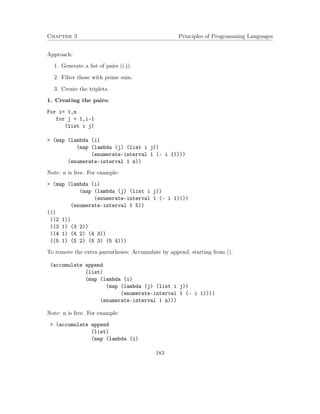
![Chapter 3 Principles of Programming Languages
(map (lambda (j) (list i j))
(enumerate-interval 1 (- i 1))))
(enumerate-interval 1 5)))
((2 1)
(3 1)
(3 2)
(4 1)
(4 2)
(4 3)
(5 1)
(5 2)
(5 3)
(5 4))
The flattening of a list using accumulate with append is popular, and can be abstracted:
Type: [[T1 - LIST(T2)]*LIST(T1) - LIST(T2)]
(define flatmap
(lambda (proc seq)
(accumulate append (list) (map proc seq))))
2. Filter the pairs with a prime sum – The filter predicate:
(define prime-sum?
(lambda (pair)
(prime? (+ (car pair) (cadr pair)))))
(prime-sum? (list 3 6))
#f
(prime-sum? (list 3 4))
#t
3. Make the triplets:
(define make-pair-sum
(lambda (pair)
(list (car pair) (cadr pair) (+ (car pair) (cadr pair)))))
The overall prime-sum-pairs procedure:
(define prime-sum-pairs
(lambda (n)
(map make-pair-sum
(filter prime-sum?
184](https://image.slidesharecdn.com/principlesofprogramminglanguages-140901163422-phpapp01/85/Principles-of-programming-languages-189-320.jpg)
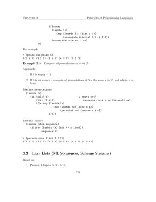
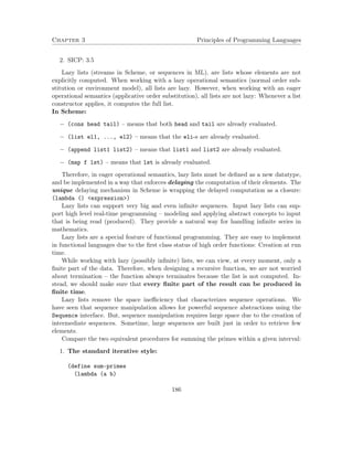
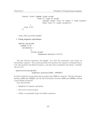
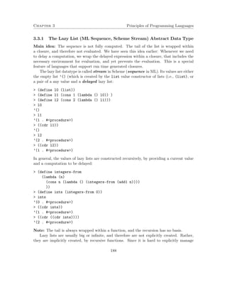
![Chapter 3 Principles of Programming Languages
these lambda wrappings and exposure, we develop a set of lazy list operations, by analogy
with lists.
3.3.1.1 Selectors of lazy lists: Head, tail, first-n-elements,nth-element
Head and tail:
Signature: head(lz-ist)
Type: [PAIR(T1,[Empty - Lazy-list]) - T1 ]
(define head car)
The tail of a lazy list is a parameter less function. Therefore, to inspect the tail, apply the
tail function. The application forces evaluation of the tail.
Signature: tail(lz-ist)
Type: [PAIR(T1,[Empty - Lazy-list]) - Lazy-list ]
(define tail
(lambda (lz-lst)
((cdr lz-lst))
))
(head l1)
1
(tail l1)
’()
(tail l2)
’(1 . #procedure)
(tail (tail ints))
’(2 . #procedure)
(car (tail (tail ints)))
2
The first n elements of a lazy-list and the nth element selectors:
(define take
(lambda (lz-lst n)
(if (= n 0)
(list)
(cons (car lz-lst)
(take (tail lz-lst) (sub1 n))))
))
(take ints 5)
’(0 1 2 3 4)
189](https://image.slidesharecdn.com/principlesofprogramminglanguages-140901163422-phpapp01/85/Principles-of-programming-languages-194-320.jpg)
![Chapter 3 Principles of Programming Languages
(take (integers-from 30) 7)
’(30 31 32 33 34 35 36)
(define nth
(lambda (lz-lst n)
(if (= n 0)
(head lz-lst)
(nth (tail lz-lst) (sub1 n)))
))
(nth ints 25)
25
Evaluation of (take (integers-from 30) 2) – using the substitution model:
applicative-eval[(take (integers-from 30) 2)] ==
applicative-eval[(integers-from 30) ] == ; eval step
applicative- eval[ (cons 30 (lambda () (integers-from (+ 30 1))))]
== (30 . (lambda () (integers-from (+ 30 1))))
applicative-eval
[(30 . (take ((lambda () (integers-from (+ 30 1)))) (- 2 1))) ] ==
; substitute, reduce
applicative-eval[ (take ((lambda () (integers-from (+ 30 1)))) (- 2 1))]
== ; eval step
applicative-eval[ (lambda () (integers-from (+ 30 1))) ] ==
; eval step
applicative-eval[ (integers-from (+ 30 1)) ] ==
;reduce step
applicative-eval[ (cons 31 (lambda () (integers-from (+ 31 1)))) ]
== ( 31 . (lambda () (integers-from (+ 31 1))))
applicative-eval
[ (31 . (take ((lambda () (integers-from (+ 31 1)))) (- 1 1))) ] ==
;reduce step
applicative-eval
[ (take ((lambda () (integers-from (+ 31 1)))) (- 1 1)) ] ==
;eval step
applicative-eval[ (lambda () (integers-from (+ 31 1))) ]
== ;eval step
applicative-eval[ (integers-from (+ 31 1)) ] ==
;reduce step
applicative-eval[ (32 . (lambda () (integers-from (+ 32 1)))) ]
== (32 . (lambda () (integers-from (+ 32 1))))
’() ==
190](https://image.slidesharecdn.com/principlesofprogramminglanguages-140901163422-phpapp01/85/Principles-of-programming-languages-195-320.jpg)
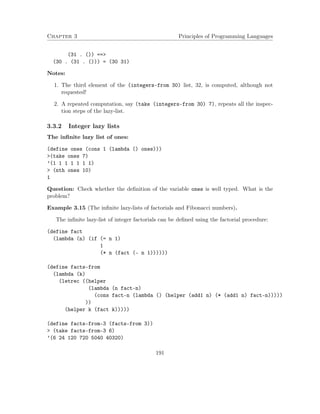
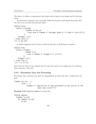
![Chapter 3 Principles of Programming Languages
Primes – Second definition: The lazy-list of primes can be created as follows:
1. Start with the integers lazy-list: [2,3,4,5,....].
2. Select the first prime: 2.
Filter the current lazy-list from all multiples of 2: [2,3,5,7,9,...]
3. Select the next element on the list: 3.
Filter the current lazy-list from all multiples of 3: [2,3,5,6,11,13,17,...].
4. i-th step: Select the next element on the list: k. Surely it is a prime, since it is not a
multiplication of any smaller integer.
Filter the current lazy-list from all multiples of k.
5. All elements of the resulting lazy-list are primes, and all primes are in the resulting
lazy-list.
(define sieve
(lambda (lz)
(cons (head lz)
(lambda ()
(sieve (lz-lst-filter (lambda (x) (not (divisible? x (head lz))))
(tail lz)))))
))
(define primes1 (sieve (integers-from 2)))
(take primes1 7)
’(2 3 5 7 11 13 17)
3.4 Continuation Passing Style (CPS) Programming
Continuation Passing Style is a programming method that assumes that every user defined
procedure f$ carries a future computation specification cont, in the form of a procedure,
that needs to apply once the computation of f$ ends.
Example 3.21. The procedures
(define square (lambda (x) (* x x)))
(define add1 (lambda (x) (+ x 1)))
turn into:
197](https://image.slidesharecdn.com/principlesofprogramminglanguages-140901163422-phpapp01/85/Principles-of-programming-languages-202-320.jpg)
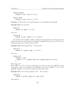
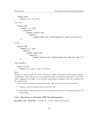
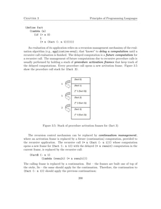
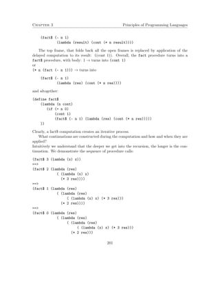
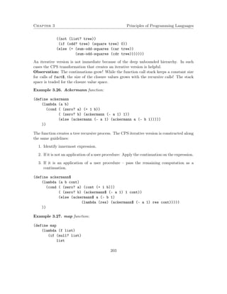
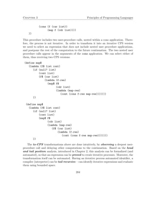
![Chapter 3 Principles of Programming Languages
3.4.2 Controlling Multiple Alternative Future Computations: Errors (Ex-ceptions),
Search and Backtracking
Example 3.28. Replace a call to error by a fail continuation:
An error (exception) marks an alternative, not planned future. Errors and exceptions
break the computation (like a goto or break in an imperative language). A call to the
Scheme primitive procedure error breaks the computation and returns no value. This is a
major problem to the type system.
In the CPS style errors can be implemented by continuations. Such a CPS procedure
carries two continuations, one for the planned future – the success continuation, and one
for the error – the fail continuation.
Signature: sumlist(li)
Purpose: Sum the elements of a number list. If the list includes a non
number element -- produce an error.
Type: [LIST - Number union ???]
(define sumlist
(lambda (li)
(cond ((null? li) 0)
((not (number? (car li))) (error non numeric value!))
(else
(+ (car li) (sumlist (cdr li)))))
))
An iterative CPS version, that uses success/fail continuations:
(define sumlist
(lambda (li)
(letrec
((sumlist$
(lambda (li succ-cont fail-cont)
(cond ((null? li) (succ-cont 0)) ;; end of list
((number? (car li)) ;; non-end, car is numeric
(sumlist$ (cdr li)
(lambda (sum-cdr) ;success continuation
(succ-cont (+ (car li) sum-cdr)))
fail-cont)) ;fail continuation
(else (fail-cont)))) ;apply the fail continuation
))
(sumlist$ li
(lambda (x) x)
(lambda ( ) (display non numeric value!))))
))
205](https://image.slidesharecdn.com/principlesofprogramminglanguages-140901163422-phpapp01/85/Principles-of-programming-languages-210-320.jpg)
![Chapter 3 Principles of Programming Languages
Note that while the success continuation is gradually built along the computation – con-structing
the stored future actions, the fail continuation is not constructed. When applied,
it discards the success continuation.
Example 3.29. Using a fail continuation for backtracking in search:
In this example, the fail continuation is used to direct the search along the tree. If the
search on some part of the tree fails, the fail continuation applies the search to another part
of the tree.
First, a non-CPS version:
Signature: leftmost-even(tree)
Purpose: Find the left most even leaf of a binary tree whose leaves are
labeled by numbers.
Type: [LIST - Number union Boolean]
Examples: (leftmost-even ’((1 2) (3 4))) == 2
(leftmost-even ’((1 1) (3 3))) == #f
(define leftmost-even
(lambda (tree)
(letrec
((iter (lambda (tree)
(cond ((null? tree) #f)
((not (list? tree))
(if (even? tree) tree #f))
(else
(let ((res-car (iter (car tree))))
(if res-car
res-car
(iter (cdr tree)))))))
))
(iter tree))
))
The leftmost-even procedure performs an exhaustive search on the tree, until an even leaf
is found. Whenever the search in the left sub-tree (the car) fails, it invokes a recursive
search on the right sub-tree – the cdr. This kind of search can be viewed as a backtracking
search policy: If the decision to search in the left sub-tree appears wrong, a retreat to the
decision point occurs, and an alternative route is selected.
The CPS version includes a success and a fail continuations. In the search decision
point, when the search is turned to the left sub-tree, the fail continuation that is passed is
the search in the right sub-tree. The fail continuation is applied when the search reaches a
leaf and fails.
206](https://image.slidesharecdn.com/principlesofprogramminglanguages-140901163422-phpapp01/85/Principles-of-programming-languages-211-320.jpg)
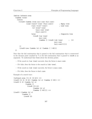
![Chapter 3 Principles of Programming Languages
(lambda (x) x)
(lambda ()
(iter$ ((3 4))
(lambda (x) x)
(lambda () #f)))))) ==*
(iter$ (2)
(lambda (x) x)
(lambda ()
(iter$ ((3 4))
(lambda (x) x)
(lambda () #f)))) ==*
( (lambda (x) x) 2) ==
2
Example 3.30. Using a success continuation for reconstructing a hierarchy:
In this example, the success/fail continuations are used for reconstructing the original
hierarchical structure, after replacing an old leaf by a new one. This is the first example
that we see, in which the CPS style simplifies the implementation. Therefore, we start
with a CPS version. Then show the more complex and less readable non-CPS version.
A CPS version:
Signature: replace-leftmost(old new tree)
Purpose: Find the left most leaf whose value is ’old’ and replace it
by new. If none, return #f.
Type: [T1*T2*LIST - LIST union Boolean]
Examples: (replace-leftmost 3 1 ’((2 2) (4 3 2 (2)) 3) ) ==
((2 2) (4 1 2 (2)) 3)
(replace-leftmost 2 1 ’((1 1) (3 3))) == #f
(define replace-leftmost
(lambda (old new tree)
(letrec
((iter$ (lambda (tree succ-cont fail-cont)
(cond ((null? tree) (fail-cont)) ; Empty tree
((not (list? tree)) ; Leaf tree
(if (eq? tree old)
(succ-cont new)
(fail-cont)))
(else ; Composite tree
(iter$ (car tree)
(lambda (car-res)
(succ-cont (cons car-res (cdr tree))))
208](https://image.slidesharecdn.com/principlesofprogramminglanguages-140901163422-phpapp01/85/Principles-of-programming-languages-213-320.jpg)
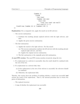
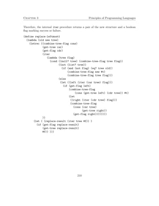
![Chapter 4
Evaluators for Functional
Programming
Sources: SICP 4.1. [1] and extensions.
Topics:
1. Abstract Syntax Parser (ASP).
2. A meta-circular evaluator for the applicative-eval operational semantics:
(a) Data structures package.
(b) Core package: Evaluation rules.
3. The Environment based operational semantics.
(a) Environment based operational semantics for functional programming.
(b) Static (Lexical) and dynamic scoping evaluation policies.
4. A meta-circular evaluator for the environment based operational semantics:
(a) Core package: Evaluation rule.
(b) Data structures package.
5. A meta-circular compiler for functional Programming: Separating syntax analysis from
execution.
Introduction on Meta-Circular Evaluators
Programming languages are used to describe problems and specify solutions. They pro-vide
means for combination and abstraction that enable hiding unnecessary details, and
211](https://image.slidesharecdn.com/principlesofprogramminglanguages-140901163422-phpapp01/85/Principles-of-programming-languages-216-320.jpg)
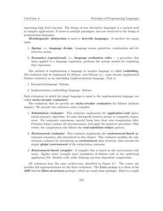
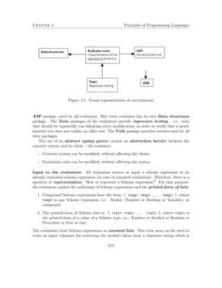
![Chapter 4 Principles of Programming Languages
The Tagged-data interface and an implementation is given below:
; Signature: attach-tag(x, tag)
; Type: [LIST*Symbol - LIST]
(define attach-tag
(lambda (x tag) (cons tag x)))
; Note that the tagged content MUST be a list!
; Signature: get-tag(tagged)
; Type: LIST - Symbol
(define get-tag (lambda (tagged) (car tagged)))
; Signature: get-content(tagged)
; Type: [LIST - T]
(define get-content
(lambda (tagged) (cdr tagged)))
Signature: tagged-data?(datum)
Type: [T - Boolean]
(define tagged-by?
(lambda (datum)
(and (list? datum) (symbol? (car datum))) ))
; Signature: tagged-by?(tagged, tag)
; Type: [T*Symbol - Boolean]
(define tagged-by?
(lambda (tagged tag)
(and (tagged-data? tagged)
(eq? (get-tag tagged) tag))))
4.1.1 The parser procedures:
For each type of expression the abstract syntax parser implements:
Predicates, to identify Scheme expressions.
Selectors to select parts of Scheme expressions.
Constructors.
1. Atomic expressions:
Atomic identifier:
216](https://image.slidesharecdn.com/principlesofprogramminglanguages-140901163422-phpapp01/85/Principles-of-programming-languages-221-320.jpg)
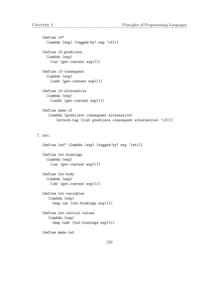
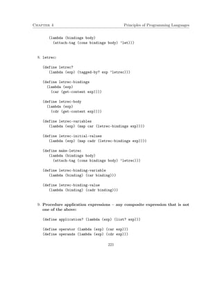
![Chapter 4 Principles of Programming Languages
(cond (( x 0) x)
(else (cond ((= x 0) 0)
(else (- x)))))
which can be optimized into
(cond (( x 0) x)
((= x 0) 0)
(else (- x)))
This is a conventional method that provides further abstraction and flexibility to lan-guages
– A compiler or interpreter does not handle explicitly the derived expressions. This
way, the evaluator provides semantics and implementation only to its core (kernel) ex-pressions.
All other (derived) expressions are defined in terms of the core expressions, and
therefore, are independent of the semantics and the implementation.
Management of derived expressions consists of:
1. Overall management:
(a) A predicate derived? that identifies derived expressions.
(b) A procedure shallow-derive that translates a derived expression into a kernel
expression without handling of nested derived expressions.
(c) A procedure derive that recursively applies shallow-derive.
2. Concrete translation: For every derived expression a shallow translation procedure
is provided. For example, if if is a derived expression, then there is a procedure
if-cond.
4.1.2.1 Overall management of derived expressions
(define derived?
(lambda (exp)
(or (if? exp) (function-definition? exp) (let? exp))))
; Type: [Scheme-exp - Scheme-exp]
; Pre-condition: exp is a derived expression.
(define shallow-derive
(lambda (exp)
(cond ((if? exp) (if-cond exp))
((function-definition? exp) (function-define-define exp))
((let? exp) (let-combination exp))
((letrec? exp) (letrec-let exp))
(else (error ’shallow-derive unhandled derivation: ~s exp)))))
223](https://image.slidesharecdn.com/principlesofprogramminglanguages-140901163422-phpapp01/85/Principles-of-programming-languages-228-320.jpg)
![Chapter 4 Principles of Programming Languages
; Type: [Scheme-exp - Scheme-exp]
; Deep derivation -- due to the recursive application
; Handling of multiple (repeated) derivation
(define derive
(lambda (exp)
(if (atomic? exp)
exp
(let ((derived-exp
(let ((mapped-derive-exp (map derive exp)))
(if (not (derived? exp))
mapped-derive-exp
(shallow-derive mapped-derive-exp)))
))
(if (equal? exp derived-exp)
exp
(derive derived-exp)) ; Repeated derivation
))))
4.1.2.2 Concrete translations
1. if as a derived expression:
(define if-cond
(lambda (exp)
(let ((predicate (if-predicate exp))
(first-actions (list (if-consequent exp)))
(second-actions (list (if-alternative exp))) )
(let ((first-clause (make-cond-clause predicate first-actions))
(second-clause (make-cond-clause ’else second-actions))
)
(make-cond (list first-clause second-clause))))
))
(if-cond ’(if ( x 0)
x
(- x)))
(cond (( x 0) x) (else (- x)))
(if-cond ’(if ( x 0)
x
(if (= x 0)
0
224](https://image.slidesharecdn.com/principlesofprogramminglanguages-140901163422-phpapp01/85/Principles-of-programming-languages-229-320.jpg)
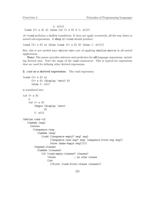
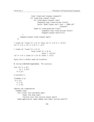
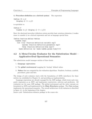
![Chapter 4 Principles of Programming Languages
4.2.1 Data Structures package
4.2.1.1 Value ADTs and their implementation
The values managed by the evaluator are numbers, booleans, symbols, procedures, pairs and
lists. Values should be distinguished from syntactic expressions, since they should not be
affected by repeated evaluation. Since Scheme syntax identifies syntactic expressions with
computed values (e.g., a quoted symbol is also a syntactic variable; a list is also a genuine
Scheme expression), the evaluator must “mark” already computed values. Therefore, all
commuted values are tagged either as procedures, or as values (including numbers and
booleans).
Indeed, algorithm applicative-eval introduced in Chapter 2 distinguishes already com-puted
values from syntactic expressions. Consider, for example, the following two evalua-tions:
applicative-eval[((lambda (x)(display x) x) (quote a))] ==
Eval:
applicative-eval[(lambda (x)(display x) x)] == Closure (x)(display x) x
applicative-eval[(quote a)] == a
Substitute: sub[x,a,(display x) x] = (display a) a
Reduce:
applicative-eval[ (display a) ] ==
Eval:
applicative-eval[display] == Code of display.
applicative-eval[’a’] == ’a’ , since ’a’ is a value of the symbol (*)
type (and not a variable!).
applicative-eval[’a’] == ’a’
and also:
applicative-eval[((lambda (lst)(car lst)) (list 1 2 3))] ==
Eval:
applicative-eval[(lambda (lst)(car lst))] == Closure (lst)(car lst)
applicative-eval[(list 1 2 3)] == List value ’(1 2 3)’
Substitute: sub[lst,’(1 2 3)’,(car lst)] = (car ’(1 2 3)’)
Reduce:
applicative-eval[ (car ’(1 2 3)’) ] ==
Eval:
applicative-eval[car] == Code of car.
applicative-eval[’(1 2 3)’] == ’(1 2 3)’ (*)
== 1
The evaluation correctly completes because applicative-eval avoids repetitive evaluations
(the lines marked by (*). Otherwise, the first evaluation would have failed with an “unbound
228](https://image.slidesharecdn.com/principlesofprogramminglanguages-140901163422-phpapp01/85/Principles-of-programming-languages-233-320.jpg)
![Chapter 4 Principles of Programming Languages
variable” error, and the second with “1 is not a procedure”. That is, if e is a value of Symbol
or Pair or List or Procedure (User or primitive), then applicative-eval[e] = e.
For that purpose, the evaluator manages value types with appropriate identification
predicates, selectors and constructors. Below we define ADTs that are implemented by
evaluator types for primitive procedures, user procedures (closures), and all otter values.
Primitive procedure values: A primitive procedure value is not a syntactic expression,
and cannot be repeatedly evaluated, as required for example, in the evaluation of ((lambda
(f)(f (list 1 2))) car). The evaluator must manage its own primitive procedure
values. The management includes the abilities to construct, identify, and retrieve the
underlying implemented code.
The Primitive-procedure ADT:
1. Constructor make-primitive-procedure: Attaches a tag to an implemented code
argument.
Type: [T - Primitive-procedure].
2. Identification predicate primitive-procedure?.
Type: [T – Boolean].
3. Selector primitive-implementation: It retrieves the implemented code from a prim-itive
procedure value.
Type: [Primitive-procedure – T].
Implementation of the Primitive-procedure ADT: Primitive procedures are repre-sented
as tagged values, using the tag primitive.
Type: [T - LIST]
(define make-primitive-procedure
(lambda (proc)
(attach-tag (list proc) ’primitive)))
Type: [T - Boolean]
(define primitive-procedure?
(lambda (proc)
(tagged-by? proc ’primitive)))
Type: [LIST - T]
(define primitive-implementation
(lambda (proc)
(car (get-content proc))))
For example:
229](https://image.slidesharecdn.com/principlesofprogramminglanguages-140901163422-phpapp01/85/Principles-of-programming-languages-234-320.jpg)
![Chapter 4 Principles of Programming Languages
(make-primitive-procedure cons)
(primitive #primitive:cons)
( (primitive-implementation (make-primitive-procedure cons))
1 2)
(1 . 2)
User procedure (closure) values: Closures should be managed as Procedure values.
The management includes the abilities to construct, identify and select (get) the pa-rameters
and the body of the closure. That is, when the evaluator evaluates a lambda
expression, it creates its own Procedure value. When a closure is applied, the selectors of
the parameters and the body are used.
The Procedure ADT:
1. make-procedure: Attaches a tag to a list of parameters and body.
Type: [LIST(Symbol)*LIST – Procedure]
2. Identification predicate compound-procedure?.
Type: [T – Boolean]
3. Selector procedure-parameters.
Type: [Procedure – LIST(Symbol)]
4. Selector procedure-body.
Type: [Procedure – LIST]
Implementation of the User-procedure ADT: User procedures (closures) are repre-sented
as tagged values, using the tag procedure.
Type: [LIST(Symbol)*LIST - LIST]
(define make-procedure
(lambda (parameters body)
(attach-tag (cons parameters body) ’procedure)))
Type: [T - Boolean]
(define compound-procedure?
(lambda (p)
(tagged-by? p ’procedure)))
Type: [LIST - LIST(Symbol)]
(define procedure-parameters
(lambda (p)
(car (get-content p))))
230](https://image.slidesharecdn.com/principlesofprogramminglanguages-140901163422-phpapp01/85/Principles-of-programming-languages-235-320.jpg)
![Chapter 4 Principles of Programming Languages
Type: [LIST - LIST]
(define procedure-body
(lambda (p)
(cdr (get-content p))))
Identifier evaluator-procedure? for either primitive or user procedure:.
Type: [LIST - Boolean]
Purpose: An identification predicate for procedures -- closures and primitive:
(define evaluator-procedure?
(lambda (p)
(or (primitive-procedure? p) (compound-procedure? p))))
Other values: Values result from the evaluation of numbers, booleans or application of
primitive procedures. The resulting values should not be repeatedly evaluated. Therefore,
the evaluator distinguishes values and evaluate them to themselves.
The Value ADT:
1. Constructor make-value.
Type: [Scheme-type-value – Evaluator-value].
2. Identification predicate value?.
Type: [T – Boolean].
3. Selector value-content.
Type: [Value – Scheme-type-value].
Implementation of the Evaluator-list ADT:
Type: [Scheme-type-value - LIST]
(define make-value
(lambda (x) (attach-tag (list x) ’value)))
Type: [T - Boolean]
(define value?
(lambda (s) (tagged-by? s ’value)))
Type: [LIST - LIST]
(define value-content
(lambda (s) (car (get-content s))))
231](https://image.slidesharecdn.com/principlesofprogramminglanguages-140901163422-phpapp01/85/Principles-of-programming-languages-236-320.jpg)
![Chapter 4 Principles of Programming Languages
4.2.1.2 The Global Environment (GE) ADT and its implementation
The Global Environment (GE) ADT represents the global environment mapping from vari-ables
to values, used by the substitution operational semantics algorithms. In addition,
in order to use primitive procedures that are already implemented in Scheme, the global
environment treats primitive procedures as defined variables.
The Global Environment ADT:
1. make-the-global-environment: Creates the single value that implements this ADT,
including Scheme primitive procedure bindings.
Type: [Empty – GE]
2. lookup-variable-value: For a given variable var, returns the value of the global-environment
on var if defined, and signs an error otherwise.
Type: [Symbol – T]
3. add-binding!: Adds a binding, i.e., a variable-value pair to the global environment
mapping. Note that add-binding is a mutator: It changes the global environment
mapping to include the new binding.
Type: [Binding – Void]
Implementation of the Global Environment ADT
I. The constructor: We know that the global environment mapping is a substitution.
Therefore, the GE ADT is implemented using the Substation ADT, which was already im-plemented
for the static type inference system, using the equations method. The Global
Environment type has a single value, named the-global-environment. This value is im-plemented
as a substitution that maps primitive-procedure names to their built-in imple-mentations,
and other defined names to their values. The Substitution operations, used
for the GE implementation are: make-sub, get-value-of-variable, extend-sub. The
implementation of the Substitution ADT is also included in the ge-adt.rkt module.
; Type: Client view: [Void - GE]
; Supplier view: [Void - LIST]
; The global environment is implemented as a substitution: A 2-element list of
; symbols and their values
(define make-the-global-environment
(lambda ()
(let* ((primitive-procedures
(list (list ’car car)
(list ’cdr cdr)
(list ’cons cons)
(list ’null? null?)
(list ’+ +)
232](https://image.slidesharecdn.com/principlesofprogramminglanguages-140901163422-phpapp01/85/Principles-of-programming-languages-237-320.jpg)
![Chapter 4 Principles of Programming Languages
(list ’* *)
(list ’/ /)
(list ’ )
(list ’ )
(list ’- -)
(list ’= =)
(list ’list list)
(list ’append append)
;; more primitives
))
(prim-variables (map car primitive-procedures))
(prim-values (map (lambda (x) (make-primitive-procedure (cadr x)))
primitive-procedures)) )
(make-sub prim-variables prim-values))
))
(define the-global-environment (make-the-global-environment))
II. The selector: The selector of the Global Environment ADT is a procedure that looks
for the value of a given variable argument in the global environment:
; Type: [Symbol - T]
(define lookup-variable-value
(lambda (var)
(get-value-of-variable the-global-environment var)))
If the global environment is not defined on the search variable, an error is triggered.
III. The mutator: The mutator of the Global Environment ADT is add-binding!, which
adds a binding, i.e., a variable-value pair, to the single GE element the-global-environment.
add-binding! applies the Substitution operation extend-sub, to the-global-environment
and the new variable-value pair, which creates a new, extended substitution. However, since
the interpreter consults the-global-environment for values of variables, add-binding!
changes the value of the-global-environment to the new extended substitution. The
mutation is implemented using the Scheme operation set!, which changes the value of an
already defined variable (assignment).
The implementation of add-binding! is not in the realm of functional pro-gramming
as it is based on mutation. The mutator is used only in the evaluation of
define forms. If the interpreted language does not include the define special operator, the
substitution interpreter system is within the functional programming paradigm.
; Type: [PAIR(Symbol,T) - Void]
(define add-binding!
233](https://image.slidesharecdn.com/principlesofprogramminglanguages-140901163422-phpapp01/85/Principles-of-programming-languages-238-320.jpg)
![Chapter 4 Principles of Programming Languages
(lambda (binding)
(let ((bvar (binding-variable binding))
(bval (binding-value binding)))
(set! the-global-environment (extend-sub the-global-environment bvar bval)))
))
;;;;;;;;;;; Bindings
; Type: [Symbol*T - PAIR)Symbol,T)]
(define make-binding
(lambda (var val)
(cons var val)))
; Type: [PAIR(Symbol,T) - Symbol]
(define binding-variable
(lambda (binding)
(car binding)))
; Type: [PAIR(Symbol,T) - T]
(define binding-value
(lambda (binding)
(cdr binding)))
Once the-global-environment is defined, we can look for values of its defined variables:
(lookup-variable-value ’cons)
’(primitive #procedure:cons)
(eq? (primitive-implementation (lookup-variable-value ’cons)) cons)
#t
( (primitive-implementation (lookup-variable-value ’cons)) 1 2)
(1 . 2)
(lookup-variable-value ’map)
. . get-value-of-variable: sub is an empty substitution or var is not a
variable of sub:
sub is ((car cdr cons null? + * / - = list append) ((primitive #procedure:car)
(primitive #procedure:cdr) (primitive #procedure:cons) (primitive #procedure:null?)
(primitive #procedure:+) (primitive #procedure:*) (primitive #procedure:/)
(primitive #procedure:) (primitive #procedure:) (primitive #procedure:-)
(primitive #procedure:=) (primitive #procedure:list)
(primitive #procedure:append)));
var is map
(add-binding! (make-binding ’map (make-primitive-procedure map)))
234](https://image.slidesharecdn.com/principlesofprogramminglanguages-140901163422-phpapp01/85/Principles-of-programming-languages-239-320.jpg)
![Chapter 4 Principles of Programming Languages
( (primitive-implementation (lookup-variable-value ’map)) - ’(1 2))
(-1 -2)
4.2.2 Core Package: Evaluation Rules
The core of the evaluator consists of the applicative-eval procedure, that implements the
applicative-eval algorithm. The main evaluation loop is created by application of closures
– user defined procedures. In that case, the evaluation process is an interplay between the
procedures applicative-eval and apply-procedure.
(applicative-eval exp) evaluates exp. It calls the abstract syntax parser for
the task of identifying language expressions. The helper procedures eval-atomic,
eval-special-form, eval-list and apply-procedure carry the actual evaluation
on the given expression. They use the abstract syntax parser selectors for getting
expression components.
(apply-procedure procedure arguments) applies procedure to arguments.
It distinguishes between
– Application of a primitive procedure: By calling apply-primitive-procedure.
– Application of a compound procedure:
It substitutes the free occurrences of the procedure parameters in its body,
by the argument values;
It sequentially evaluates the forms in the procedure body.
4.2.2.1 Main evaluator loop:
The evaluator application is preceded by deep replacement of all derived expressions by
their defining expressions.
(define derive-eval
(lambda (exp)
(applicative-eval (derive exp))))
The input to the evaluator is either a syntactically legal kernel Scheme expression
(the evaluator does not check syntax correctness) or an evaluator value, i.e., an already
evaluated Scheme expression. The evaluator does not support the letrec special operator.
Therefore, the input expression cannot include inner recursive procedures.
; Type: [(Scheme-exp union Evaluator-value) - (Evaluator-value union Scheme-type)]
; Evaluator-value is a Scheme-type value, that is marked as a value. Procedures
; (user or primnitive) are distinguished from other values. Numbers and
; Booleans are also marked.
235](https://image.slidesharecdn.com/principlesofprogramminglanguages-140901163422-phpapp01/85/Principles-of-programming-languages-240-320.jpg)
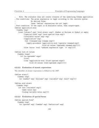
![Chapter 4 Principles of Programming Languages
(lambda (exps)
(let ((vals (map (lambda(e) (applicative-eval e))
exps)))
(last vals))
))
Auxiliary procedures:
(define true?
(lambda (x)
(not (false? x))))
(define false?
(lambda (x)
(or (eq? x #f) (equal? x ’(value #f)))))
4.2.2.4 Value identification
(define evaluator-value?
(lambda (val) (or (value? val)
(primitive-procedure? val) (compound-procedure? val))))
4.2.2.5 Evaluation of applications
apply-procedure evaluates a form (a non-special combination). Its arguments are an
Evaluator-procedure, i.e., a tagged procedure value that is created by the evaluator, and
already evaluated arguments (the applicative-eval procedure first evaluates the argu-ments
and then calls apply procedure). The argument values are either atomic (numbers
or booleans) or tagged evaluator values. If the procedure is not primitive, apply-procedure
carries out the substitute-reduce steps of the applicative-eval algorithm.
; Type: [Evaluator-procedure*LIST - Evaluator-value union Scheme-type]
(define apply-procedure
(lambda (procedure arguments)
(cond ((primitive-procedure? procedure)
(apply-primitive-procedure procedure arguments))
((compound-procedure? procedure)
(let ((parameters (procedure-parameters procedure))
(body (rename (procedure-body procedure))))
(eval-sequence
(substitute body parameters arguments))))
(else (error ’apply Unknown procedure type: ~s procedure)))))
238](https://image.slidesharecdn.com/principlesofprogramminglanguages-140901163422-phpapp01/85/Principles-of-programming-languages-243-320.jpg)
![Chapter 4 Principles of Programming Languages
Primitive procedure application: Primitive procedures are tagged data values used
by the evaluator. Therefore, their implementations must be retrieved prior to application
(using the selector primitive-implementation). The arguments are values, evaluated by
applicative-eval. Therefore, the arguments are values of the interpreter, i.e., tagged
data values – for values, primitive procedures and closures. The primitive procedure imple-mentation
should receive only the value-content. The result of the application should be
wrapped as an evaluator value.
; Type: [Evaluator-primitive-procedure*LIST - Evaluator-value]
; Retrieve the primitive implementation, retrieve content of the evaluator value
; arguments, apply and create a new evaluator value.
(define apply-primitive-procedure
(lambda (proc args)
(make-value
(apply (primitive-implementation proc)
(map (lambda (arg)
(cond ((evaluator-value? arg) (value-content arg))
((primitive-procedure? arg) (primitive-implementation arg))
((compound-procedure? arg)
(error ’apply-primitive-procedure
primitive-appliled-to-evaluator-procedure: ~s arg))
(else arg)))
args)))
))
apply is a Scheme primitive procedure that applies a procedure on its arguments:
(apply f e1 ... en) == (f e1 ... en).
Its type is: [[T1*...*Tn – T]*LIST – T]. For a procedure of n parameters, the list
argument must be of length n, with corresponding types.
Problem with applying high order primitive procedures: The applicative-eval
evaluator cannot apply high order Scheme primitive procedures like map, apply. The reason
is that such primitives expect a closure as an argument. But in order to create a Scheme
closure for a given lambda expression, applicative-eval has to explicitly call Scheme to
evaluate the given expression. Since applicative-eval is implemented in Scheme, it means
that the Scheme interpreter has to open a new Scheme interpreter process. Things would
have been different, if Scheme would have provided a primitive for closure creation. But,
since lambda, the value constructor of procedures is a special operator, Scheme does not
enables us to retrieve its implementation, and therefore we cannot intentionally apply it to
given parameters and body.
239](https://image.slidesharecdn.com/principlesofprogramminglanguages-140901163422-phpapp01/85/Principles-of-programming-languages-244-320.jpg)
![Chapter 4 Principles of Programming Languages
4.2.2.6 Substitution and renaming
Substitution: The substitute procedure substitutes free variable occurrences in an ex-pression
by given values. The expression can be either a Scheme expression or a Scheme
value. substitute is preceded by renaming, and therefore, the substituted variables do not
occur as bound in the given expression (all bound variables are already renamed).
The substitute operation is part of the Substitution ADT. It is the same procedure as
the one used in the type inference system for the equations method, only adapted to the
case of Scheme expressions and Scheme values.
;Signature: substitute(sub,expr)
; Purpose: Consistent replacement of all FREE occurrences of the substitution
; variables in ’expr’ by the values of the substitution, respectively.
; ’expr’ is a Scheme expression or an Evaluator value.
;Type: Client view: [Substitution*Scheme-expression union Evaluator-value -
; Scheme-expression union Evaluator-value]
; Supplier view: [LIST*(LIST union Symbol) - LIST union Symbol]
;Example: (substitute
; (make-sub ’(x y z) ’(3 4 (lambda (x1)(+ x1 1))))
; ’(lambda (x2)(+ x2 y))) ) == (lambda (x2)(+ x2 4))
; Pre-conditions: (1) substitution is not performed on ’define’ or ’let’
; expressions or on expressions containing such sub-expressions.
; (2) ’expr’ is already renamed. Therefore, the substitution
; variables have no bound occurrences in expr.
(define substitute
(lambda (expr variables values)
(if (evaluator-value? expr)
(substitution-application-to-value (make-sub variables values) expr)
(substitution-application-to-expr (make-sub variables values) expr))
))
(define substitution-application-to-expr
(lambda (sub expr)
(cond ((empty-sub? sub) expr)
((or (number? expr) (boolean? expr) (quoted? expr)) expr)
(else (let ((vars (get-variables sub))
(values (get-values sub)))
(cond ((variable? expr)
(if (member expr vars)
(get-value-of-variable sub expr)
expr))
(else
240](https://image.slidesharecdn.com/principlesofprogramminglanguages-140901163422-phpapp01/85/Principles-of-programming-languages-245-320.jpg)
![Chapter 4 Principles of Programming Languages
; expression is a list of expressions, lambda, application, cond.
(map (lambda (e)
(substitute e vars values))
expr))))))
))
(define substitution-application-to-value
(lambda (sub val-expr)
(let ((vars (get-variables sub))
(values (get-values sub)))
(cond ((primitive-procedure? val-expr) val-expr)
((value? val-expr)
(if (atomic? (value-content val-expr))
val-expr
(make-value (map (lambda (e) (substitute e vars values))
(value-content val-expr)))))
((compound-procedure? val-expr)
(make-procedure (procedure-parameters val-expr)
(map (lambda (e) (substitute e vars values))
(procedure-body val-expr))))))
))
Renaming: rename performs consistent renaming of bound variables.
Signature: rename(exp)
Purpose: Consistently rename bound variables in ’exp’.
Type: [(Scheme-exp union Evaluator-value) - (Scheme-exp union Evaluator-value)]
(define rename
(letrec ((make-new-names
(lambda (old-names)
(if (null? old-names)
(list)
(cons (gensym) (make-new-names (cdr old-names))))))
(replace
(lambda (val-exp)
(cond ((primitive-procedure? val-exp) val-exp)
((value? val-exp)
(if (atomic? (value-content val-exp))
val-exp
(make-value (map rename (value-content val-exp)))))
((compound-procedure? val-exp)
241](https://image.slidesharecdn.com/principlesofprogramminglanguages-140901163422-phpapp01/85/Principles-of-programming-languages-246-320.jpg)
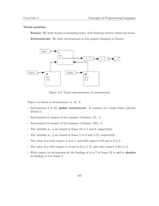
![Chapter 4 Principles of Programming Languages
Operations on environments and frames:
1. Environment operations:
Constructor:
Environment extension: Env*Frame - Env
f1; f2; :::; fn f = f; f1; f2; :::; fn
Selectors:
Find variable value: Variable*Env - Scheme-type
E(x) = fi(x), where for 1 j i; fj(x) is undefined
(= unbound)
First-frame: Env - Frame
f1; f2; :::; fn 1 = f1
Enclosing-environment: Env - Env
f1; f2; :::; fn enclosing = f2; :::; fn
Operation:
Add a binding: Env*Binding - Env
Pre-condition: f1(x)=unbound
f1; f2; :::; fn x; val = f2; :::; fn (f1 x; val )
2. Frame operations:
Constructor: A frame is constructed from variable and value sequences:
( var1; :::; varn ; val1; :::; valn ) ) [ var1; :::; varn ! val1; :::; valn
]
Selector: Variable value in a frame:
f(x) or UNBOUND, if x is not defined in f.
4.3.1.2 The closure data structure
A closure in the environment model is a pair of a procedure code, i.e., parameters and
body, and an environment. It is denoted Closure parameters body, environment. The
components of a closure cl are denoted clparameters; clbody; clenvironment.
246](https://image.slidesharecdn.com/principlesofprogramminglanguages-140901163422-phpapp01/85/Principles-of-programming-languages-251-320.jpg)
![Chapter 4 Principles of Programming Languages
4.3.2 The Environment Model Evaluation Algorithm
Signature: env-eval(e,env)
Purpose: Evaluate Scheme expressions using an Environment data structure
for holding parameter bindings in procedure applications..
Type: Scheme-exp*Env - Scheme type
env-eval[e,env] =
I. atomic?(e):
1. number?(e) or boolean?(e): env-eval[e,env] = e.
2. variable?(e):
a. If env(e) is defined, env-eval[e,env] = env(e).
b. Otherwise: e must be a variable denoting a Primitive procedure:
env-eval[e,env] = built-in code for e.
II. composite?(e): e = (e0 e1 ... en) (n = 0):
1. e0 is a Special Operator:
env-eval[e,env] is defined by the special evaluation rule of
e0 (see below).
2. a. Evaluate: Compute env-eval[ei,env] = e1’ for all e1.
b. primitive-procedure?(e0’):
env-eval[e,env] = system application e0’(e1’,...,e1’)
c. user-procedure?(e0’): e0’ is a closure.
i. Environment-extension:
new-env = e0’environment*[e0’parameters - e1’,...,en’]
ii. Reduce: If e0’body = b1,...,bm,
env-eval[b1,new-env],...,env-eval[bm1,new-env]
env-eval[e,env] = env-eval[bm,new-env]
Special operator evaluation rules:
1. e = (define x e1):
GE = GE*x,env-eval[e1,GE]
2. e = (lambda (x1 x2 ... xn) b1 ... bm) at least one bi is required:
env-eval[e,env] = Closure (x1,...,xn) (b1,...,bm), env)
3. e = (quote e1):
env-eval[e,env] = e1
4. e = (cond (p1 e11 ... e1k1) ... (else en1 ... enkn))
If true?(env-eval[p1,env]) (!= #f in Scheme):
env-eval[e11,env],env-eval[e12,env],...
247](https://image.slidesharecdn.com/principlesofprogramminglanguages-140901163422-phpapp01/85/Principles-of-programming-languages-252-320.jpg)
![Chapter 4 Principles of Programming Languages
env-eval[e,env] = env-eval[e1k1,env]
otherwise, continue with p2 in the same way.
If for all pi-s env-eval[pi,env] = #f:
env-eval[en1,env],env-eval[en2,env],...
env-eval[e,env] = env-eval[enkn,env]
5. e = (if p con alt)
If true?(env-eval[p,env]):
then env-eval[e,env] = env-eval[con,env]
else env-eval[e,env] = env-eval[alt,env]
6. e = (begin e1,...,en)
env-eval[e1,env],...,env-eval[en1,env].
env-eval[e,env] = env-eval[en,env].
Notes:
1. A new environment is created only when the computation reduces to the evaluation
of a closure body. Therefore, there is a 1:many correspondence between environments
and lexical scopes.
An environment corresponds to a lexical scope (i.e., a procedure definition body).
A lexical scope can correspond to multiple environments!
2. env-eval consults or modify the environment structure in the following steps:
(a) Creation of a compound procedure (closure): Evaluation of a lambda form (and
of a let form).
(b) Application of a compound procedure (closure) – the only way to add a frame
(also in the evaluation of a let form).
(c) Evaluation of define form – adds a binding to the global environment.
(d) Evaluation of a variable.
3. De-allocation of frames: Is not handled by the environment evaluator (left to the
storage-allocation strategy of an interpreter). When the evaluation of a procedure
body is completed, if the new frame is not included within a value of some variable
of another environment, the new frame turns into garbage and disappears from the
environments structure.
248](https://image.slidesharecdn.com/principlesofprogramminglanguages-140901163422-phpapp01/85/Principles-of-programming-languages-253-320.jpg)
![Chapter 4 Principles of Programming Languages
4.3.2.1 Substitution model vs. environment model
It can be proved:
For scheme expressions in the functional programming paradigm (no destructive operations):
applicative-eval[e] = env-eval[e,GE].
The two evaluation algorithms differ in the application step II.2.c.
The substitute-reduce steps in applicative-eval: Rename the procedure body and
the evaluated arguments, substitute the parameters by the evaluated arguments, and
evaluate the substituted body,
is replaced by
the environment extension step in env-eval: Bind the parameters to the evaluated
arguments, extend the environment of the procedure, and evaluate the procedure body
with respect to this new environment.
The effect is that explicit substitution in applicative-eval is replaced by variable bindings
in an environment structure that tracks the scope structure in the code:
The environment structure in a computation of env-eval is always isomorphic to
the scope structure in the code. Therefore, the computations are equivalent.
Scheme applications are implemented using the environment model. This result enables us
to run functional Scheme code as if it runs under applicative-eval.
4.3.2.2 Environment diagrams
An environment diagram is a data structure (type) that is associated with a computation
of (or part of) env-eval. Its values carry the following data:
1. All environments constructed during the computation. Each environment is identified
by its (unique) name, and its serial number in the order of environment construction.
Usually, the names are E1, E2, ..., where the environment named Ei is the i-th in
the construction order. The global environment is named GE.
2. Each environment is associated with a lexical block in the evaluated code, and its
code.
3. Each environment has a return control link and a return value. The return control
link points to the environment where computation continues, once the evaluation of
the code of the environment is over. The return value is the value of the evaluation of
the code of the environment.
249](https://image.slidesharecdn.com/principlesofprogramminglanguages-140901163422-phpapp01/85/Principles-of-programming-languages-254-320.jpg)
![Chapter 4 Principles of Programming Languages
Environment diagrams are visualized, using the visual notation of environments. This no-tation
is enriched with:
1. Environment names.
2. The lexical blocks of the environments (optional) and their codes. The global scope is
marked B0 and inner scopes are marked B1, B2, .... For example:
(define square (lambda(x) (* x x) B1)) B0
3. Return control links and return values. These links are marked with dashed arrows.
Each dashed arrow points to the name of the environment that the return control link
points to, and to the return value of the environment.
Scoping and control structures in environment diagrams: The tree structured lexical
scopes are reflected in the tree structure of frames in an environment diagram. The sequential
computation is reflected in the linear order of frames. Therefore, the environment links create
a tree structure, while the return control links create a linear order.
Example 4.1.
env-eval[(define square (lambda(x)(* x x))),GE] ==
GE(square) = env-eval[(lambda(x)(* x x)),GE] =
= Closure (x)(* x x),GE
Lexical blocks: (define square (lambda(x) (* x x) B1)) B0
Evaluating this form with respect to the global environment includes evaluation of the
lambda form, and binding square to the created closure, in the global environment. The
resulting environment diagram is described in Figure 4.3. Note that the closure carries the
Figure 4.3
Global Environment.
250](https://image.slidesharecdn.com/principlesofprogramminglanguages-140901163422-phpapp01/85/Principles-of-programming-languages-255-320.jpg)
![Chapter 4 Principles of Programming Languages
Note: Since the Global Environment is static, and always corresponds to the global scope
B0, the B0 is usually omitted from the diagram.
Example 4.2. Continuing Example 4.1:
env-eval[(square 5), GE] ==
env-eval[square, GE] == Closure (x)(* x x), GE
env-eval[5, GE] == 5
Denote: E1 = GE * make-frame([x],[5])
env-eval[ (* x x), E1 ] ==
env-eval[*, E1] == Primitive procedure *
env-eval[x, E1] == 5
env-eval[x, E1] == 5
25
The resulting environment diagram is described in Figure 4.4.
Figure 4.4
Example 4.3. Continuing Example 4.1, assume that the following definitions are already
evaluated (with respect to the Global Environment):
(define sum-of-squares
(lambda (x y)
(+ (square x) (square y))))
(define f
(lambda (a)
(sum-of-squares (+ a 1) (* a 2))))
Lexical blocks:
(define sum-of-squares (lambda (x y) (+ (square x) (square y)) B2))
251](https://image.slidesharecdn.com/principlesofprogramminglanguages-140901163422-phpapp01/85/Principles-of-programming-languages-256-320.jpg)
![Chapter 4 Principles of Programming Languages
(define f (lambda (a) (sum-of-squares (+ a 1) (* a 2)) B3))
env-eval[(f 5), GE] ==
env-eval[f, GE] ==
Closure (a) (sum-of-squares (+ a 1) (* a 2)), GE
env-eval[5, GE] == 5
Denote: E1 = GE * make-frame([a],[5])
env-eval[ (sum-of-squares (+ a 1) (* a 2)), E1 ] ==
env-eval[sun-of-squares, E1] ==
Closure (x y) (+ (square x) (square y)), GE
env-eval[(+ a 1), E1] ==* 6
env-eval[(* a 2), E1] ==* 10
Denote: E2 = GE * make-frame([x,y],[6,10])
env-eval[ (+ (square x) (square y)), E2 ] ==
env-eval[+, E2] == Primitive procedure +
env-eval[(square x), E2] ==
env-eval[square, E2] == Closure (x) (* x x), GE
env-eval[x, E2] == 6
Denote: E3 = GE * make-frame([x],[6])
env-eval[(* x x), E3] ==* 36
env-eval[(square y), E2] ==
env-eval[square, E2] == Closure (x) (* x x), GE
env-eval[y, E2] == 10
Denote: E4 = GE * make-frame([x],[10])
env-eval[(* x x), E4] ==* 100
136
The resulting environment diagram is described in Figure 4.5.
Example 4.4. Assume that the definitions below are already evaluated. Lexical blocks are
marked on the definitions.
(define sum
(lambda (term a next b)
(if ( a b) 0 (+ (term a) (sum term (next a) next b))) B1))
(define sum-integers (lambda (a b) (sum identity a add1 b) B2))
(define identity (lambda (x) x B3))
(define sum-cubes (lambda (a b) (sum cube a add1 b) B4))
(define cube (lambda (x) (* x x x) B5))
Describe the computation of the following expressions by an environment diagram:
252](https://image.slidesharecdn.com/principlesofprogramminglanguages-140901163422-phpapp01/85/Principles-of-programming-languages-257-320.jpg)
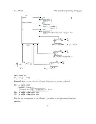
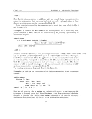
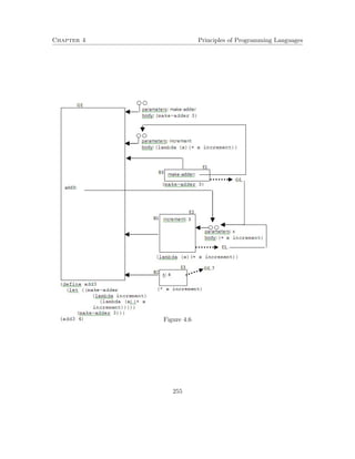
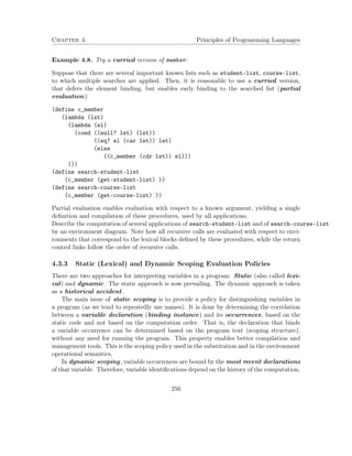
![Chapter 4 Principles of Programming Languages
i.e., on dynamic runs of a program. In different runs, a variable occurrence can be bound
by different declarations, based on the computation.
The env-eval algorithm can be adapted into dynamic-env-eval, that operates under
the dynamic evaluation policy, by unifying the enclosing-environment and the return control
links. The modifications are:
1. A closure does not carry an environment (that corresponds to the lexical scope of the
definition).
If e = (lambda (x1 x2 ... xn) b1 ... bm):
dynamic-env-eval[e,env] = make-procedure((x1,...,xn),(b1,...,bm))
2. A closure application is evaluated with respect to its calling environment:
Step II.2.c of dynamic-env-eval[e, env]:
II. composite?(e): e = (e0 e1 ... en) (n = 0):
1. e0 is a Special Operator:
env-eval[e,env] is defined by the special evaluation rule of
e0 (see below).
2. a. Evaluate: Compute env-eval[ei,env] = e1’ for all e1.
b. primitive-procedure?(e0’):
env-eval[e,env] = system application e0’(e1’,...,e1’)
c. user-procedure?(e0’): e0’ is a closure.
i. Environment-extension:
new-env = env * [e0’parameters - e1’,...,e1’] (***)
ii. Reduce: If e0’body = b1,...,bm,
env-eval[b1,new-env],...,env-eval[bm1,new-env]
env-eval[e,env] = env-eval[bm,new-env]
Note that in dynamic scoping evaluation, the tree-like environment structure disappears,
leaving only the sequential frames structure of the return-control-links. Lexical scope does
not exist, and free variable occurrences in a procedure are bound by the most recent declara-tions,
depending on the computation history. That is, bindings of free variable occurrences
are determined by the calling scopes. Procedure calls that reside in different scopes, might
have different declarations that bind free occurrences. Clearly, this cannot be done at com-pile
time (because calling environments exist only at runtime), which is why this evaluation
policy is called dynamic scoping evaluation. The impact is that in dynamic evaluation free
variables are not used. All necessary scope information is passed as procedure parameters,
yielding long parameter sequences.
257](https://image.slidesharecdn.com/principlesofprogramminglanguages-140901163422-phpapp01/85/Principles-of-programming-languages-262-320.jpg)
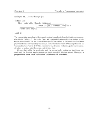
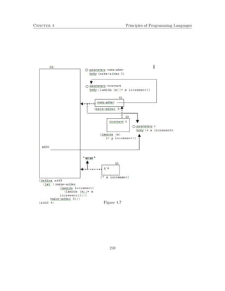
![Chapter 4 Principles of Programming Languages
Example 4.10.
(define f
(lambda (x) (a x x)))
; ’x’ is bound by the parameter of ’f’, while ’a’ is bound by
; declarations in the global scope (the entire program)
(define g
(lambda (a x) (f x)))
(define a +)
; An ’a’ declaration in the global scope.
(g * 3)
6
In lexical scoping, the a occurrence in the body of f is bound by the a declaration in the
global scope, whose value is the primitive procedure +. Every application of f is done with
respect to the global environment, and therefore, a is evaluated to primitive +. However,
in a dynamic scoping discipline, the a is evaluated with respect to the most recent frame
where it is defined – the first frame of g’s application, where it is bound to primitive *.
Therefore,
env-eval[(g * 3),GE] == 6
while
dynamic-env-eval[(g * 3),GE] == 9
Example 4.11.
Assume the definitions of Example 4.10.
(let ( (a 3))
(f a))
6
env-eval[(let ((a 3)) (f a)),GE] == 6
while
dynamic-env-eval[(let ( (a 3)) (f a)),GE] == runtime error: 3 is not a procedure.
Example 4.12.
(define init 0)
(define 1+ (lambda(x)(+ x 1)))
(define f
(lambda (f1)
(let ((f2 (lambda () (f1 init))))
(let ((f1 1+)
260](https://image.slidesharecdn.com/principlesofprogramminglanguages-140901163422-phpapp01/85/Principles-of-programming-languages-265-320.jpg)
![Chapter 4 Principles of Programming Languages
(init 1))
(f2) ))
))
Which is identical to:
(define f
(lambda (f1)
( (lambda (f2)
( (lambda (f1 init) (f2) )
1+ 1))
(lambda () (f1 init)))
))
Now evaluate:
(f (lambda (x) (* x x)))
env-eval[(f (lambda (x) (* x x)))] == 0
dynamic-env-eval[(f (lambda (x) (* x x)))] == 2
Why?
Summary of the evaluation policies discussed so far:
1. The substitution model (applicative/normal) and the environment model implement
the static scoping approach;
(a) Applicative order and environment model – eager evaluation approach.
(b) Normal order – lazy evaluation approach.
2. (a) The (applicative) env-eval algorithm has a normal version (not presented). It
extends the applicative version, i.e., no contradiction.
(b) The applicative-eval and the env-eval are equivalent.
(c) All algorithms are equivalent on the intersection of their domains.
(d) Cost of the normal wider domain: Lower efficiency, and complexity of implemen-tation
of the normal policy.
3. The static-dynamic scoping policies: Contradicting results. The algorithm dynamic-env-eval
is not equivalent to the other 3 algorithms.
(a) The major drawback of the dynamic evaluation semantics is that programs cannot
use free variables, since it is not known to which declarations they will be bound
during computation. Indeed, in this discipline, procedures usually have long
parameter lists. Almost no modern language uses dynamic evaluation. Logo and
Emacs Lisp are some of the few languages that use dynamic evaluation.
261](https://image.slidesharecdn.com/principlesofprogramminglanguages-140901163422-phpapp01/85/Principles-of-programming-languages-266-320.jpg)
![Chapter 4 Principles of Programming Languages
(b) The implementation of dynamic evaluation is simple. Indeed, traditional LISPs
used dynamic binding.
Conclusion: Programs can be indifferent to whether the operational semantics is one of
the applicative, normal or environment models. But, programs cannot be switched between
the above algorithms and the dynamic scoping policy.
4.4 A Meta-Circular Evaluator for the Environment Based
Operational Semantics
(Environment-evaluator package in the course site.)
Recall the meta-circular evaluator that implements the substitution model for functional
programming. It has the following packages:
1. Evaluation rules.
2. Abstract Syntax Parser (ASP) (for kernel and derived expressions).
3. Data structure package, for handling procedures and the Global environment.
The evaluator for the environment based operational semantics implements the env-eval
algorithm. Therefore, the main modification to the substitution model interpreter involves
the management of the data structures: Environment and Closure. The ASP package is the
same for all evaluators. We first present the evaluation rules package, and then the data
structures package.
4.4.1 Core Package: Evaluation Rules
The env-eval procedure takes an additional argument of type Env, which is consulted when
bindings are defined, and used when a closure is created or applied.
As in the substitution evaluator, there is a single environment that statically exist: The
global environment. It includes bindings to the built-in primitive procedures.
4.4.1.1 Main evaluator loop:
(SICP 4.1.1).
The core of the evaluator, as in the substitution model evaluator, consists of the env-eval
procedure, that implements the environment model env-eval algorithm. Evaluation is
preceded by deep replacement of derived expressions.
; Type: [Scheme-exp - Scheme-type]
(define derive-eval
(lambda (exp)
(env-eval (derive exp) the-global-environment)))
262](https://image.slidesharecdn.com/principlesofprogramminglanguages-140901163422-phpapp01/85/Principles-of-programming-languages-267-320.jpg)
![Chapter 4 Principles of Programming Languages
The input to the environment based evaluator is a syntactically legal Scheme expres-sion
(the evaluator does not check syntax correctness), and an environment value. The
evaluator does not support the letrec special operator. Therefore, the input expression
cannot include inner recursive procedures.
; Type: [Scheme-exp*Env - Scheme-type]
; (Number, Boolean, Pair, List, Evaluator-procedure)
; Note that the evaluator does not create closures of the
; underlying Scheme application.
; Pre-conditions: The given expression is legal according to the concrete syntax.
; Inner ’define’ expressions are not legal.
(define env-eval
(lambda (exp env)
(cond ((atomic? exp) (eval-atomic exp env))
((special-form? exp) (eval-special-form exp env))
((application? exp)
(apply-procedure (env-eval (operator exp) env)
(list-of-values (operands exp) env)))
(else (error ’eval unknown expression type: ~s exp)))))
; Type: [LIST - LIST]
(define list-of-values
(lambda (exps env)
(if (no-operands? exps)
’()
(cons (env-eval (first-operand exps) env)
(list-of-values (rest-operands exps) env)))))
4.4.1.2 Evaluation of atomic expressions
(define atomic?
(lambda (exp)
(or (number? exp) (boolean? exp) (variable? exp) (null? exp))))
(define eval-atomic
(lambda (exp env)
(if (or (number? exp) (boolean? exp) (null? exp))
exp
(lookup-variable-value env exp))))
263](https://image.slidesharecdn.com/principlesofprogramminglanguages-140901163422-phpapp01/85/Principles-of-programming-languages-268-320.jpg)
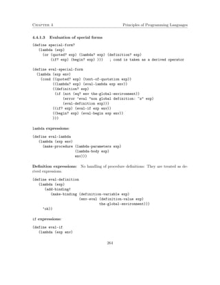
![Chapter 4 Principles of Programming Languages
(if (true? (env-eval (if-predicate exp) env))
(env-eval (if-consequent exp) env)
(env-eval (if-alternative exp) env))))
Sequence evaluation:
(define eval-begin
(lambda (exp env)
(eval-sequence (begin-actions exp) env)))
(define eval-sequence
(lambda (exps env)
(let ((vals (map (lambda (e)(env-eval e env)) exps)))
(last vals))))
Auxiliary procedures:
(define true?
(lambda (x) (not (eq? x #f))))
(define false?
(lambda (x) (eq? x #f)))
4.4.1.4 Evaluation of applications
apply-procedure evaluates a form (a non-special combination). Its arguments are an
Evaluator-procedure, i.e., a tagged procedure value that is created by the evaluator, and
already evaluated arguments (the env-eval procedure first evaluates the arguments and
then calls apply procedure). The argument values are either Scheme values (numbers,
booleans, pairs, lists, primitive procedure implementations) or tagged evaluator values of
procedures or of primitive procedures. If the procedure is not primitive, apply-procedure
carries out the environment-extension-reduce steps of the env-eval algorithm.
; Type: [Evaluator-procedure*LIST - Scheme-type]
(define apply-procedure
(lambda (procedure arguments)
(cond ((primitive-procedure? procedure)
(apply-primitive-procedure procedure arguments))
((compound-procedure? procedure)
(let* ((parameters (procedure-parameters procedure))
(body (procedure-body procedure))
(env (procedure-environment procedure))
265](https://image.slidesharecdn.com/principlesofprogramminglanguages-140901163422-phpapp01/85/Principles-of-programming-languages-270-320.jpg)
![Chapter 4 Principles of Programming Languages
(new-env (extend-env (make-frame parameters arguments) env)))
(eval-sequence body new-env)))
(else (error ’apply unknown procedure type: ~s procedure)))))
Primitive procedure application: Primitive procedures are tagged data values used
by the evaluator. Therefore, their implementations must be retrieved prior to application
(using the selector primitive-implementation). The arguments are values, evaluated
by env-eval. Therefore, the arguments are either Scheme numbers, booleans, pairs, lists,
primitive procedure implementations, or tagged data values of procedures or of primitive
procedures.
; Type: [Evaluator-primitive-procedure*LIST - Scheme-type]
; Purpose: Retrieve the primitive implementation, and apply to args.
(define apply-primitive-procedure
(lambda (proc args)
(apply (primitive-implementation proc) args)))
4.4.2 Data Structures Package
4.4.2.1 Procedure ADTs and their implementation
The environment based evaluator manages values for primitive procedure, and for user
procedure. User procedures are managed since the application mechanism must retrieve
their parameters, body and environment. Primitive procedures are managed as values since
the evaluator has to distinguish them from user procedures. For example, when evaluating
(car (list 1 2 3)), after the Evaluate step, the evaluator must identify whether the
value of car is a primitive implementation or a user procedure1.
Primitive procedure values: The ADT for primitive procedures is the same as in the
substitution evaluator.
The ADT:
1. Constructor make-primitive-procedure: Attaches a tag to an implemented code
argument.
Type: [T - Primitive-procedure].
2. Identification predicate primitive-procedure?.
Type: [T – Boolean].
3. Selector primitive-implementation: It retrieves the implemented code from a prim-itive
procedure value.
Type: [Primitive-procedure – T].
1In the substitution evaluator there was also the problem of preventing repeated evaluations.
266](https://image.slidesharecdn.com/principlesofprogramminglanguages-140901163422-phpapp01/85/Principles-of-programming-languages-271-320.jpg)
![Chapter 4 Principles of Programming Languages
Implementation of the Primitive-procedure ADT: Primitive procedures are repre-sented
as tagged values, using the tag primitive.
Type: [T -- LIST]
(define make-primitive-procedure
(lambda (proc)
(attach-tag (list proc) ’primitive)))
Type: [T - Boolean]
(define primitive-procedure?
(lambda (proc)
(tagged-by? proc ’primitive)))
Type: [LIST - T]
(define primitive-implementation
(lambda (proc)
(car (get-content proc))))
User procedure (closure) values: The tagged Procedure values of env-eval are sim-ilar
to those of applicative-eval. The only difference involves the environment compo-nent,
used both in construction and in selection.
The ADT:
1. make-procedure: Attaches a tag to a list of parameters and body.
Type: [LIST(Symbol)*LIST*Env – Procedure]
2. Identification predicate compound-procedure?.
Type: [T – Boolean]
3. Selector procedure-parameters.
Type: [Procedure – LIST(Symbol)]
4. Selector procedure-body.
Type: [Procedure – LIST]
5. Selector procedure-environment.
Type: [Procedure – Env]
Implementation of the User-procedure ADT: User procedures (closures) are repre-sented
as tagged values, using the tag procedure.
Type: [LIST(Symbol)*LIST*Env - LIST]
(define make-procedure
(lambda (parameters body env)
267](https://image.slidesharecdn.com/principlesofprogramminglanguages-140901163422-phpapp01/85/Principles-of-programming-languages-272-320.jpg)
![Chapter 4 Principles of Programming Languages
(attach-tag (list parameters body env) ’procedure)))
Type: [T - Boolean]
(define compound-procedure?
(lambda (p)
(tagged-by? p ’procedure)))
Type: [LIST - LIST(Symbol)]
(define procedure-parameters
(lambda (p)
(car (get-content p))))
Type: [LIST - LIST]
(define procedure-body
(lambda (p)
(cadr (get-content p))))
Type: [LIST - Env]
(define procedure-environment
(lambda (p)
(caddr (get-content p))))
Type: [T - Boolean]
Purpose: An identification predicate for procedures -- closures and primitive:
(define procedure?
(lambda (p)
(or (primitive-procedure? p) (compound-procedure? p))))
4.4.2.2 Environment related ADTs and their implementations:
The environment based operational semantics has a rich environment structure. Therefore,
the interface to environments includes three ADTs: Env, Frame, Binding. The Env ADT is
implemented on top of the Frame ADT, and both are implemented on top of the Binding
ADT. Frame is implemented on top of the Substitution ADT.
The Env ADT and its implementation:
The ADT:
1. make-the-global-environment(): Creates the single value that implements this ADT,
including Scheme primitive procedure bindings.
Type: [Void – GE]
268](https://image.slidesharecdn.com/principlesofprogramminglanguages-140901163422-phpapp01/85/Principles-of-programming-languages-273-320.jpg)
![Chapter 4 Principles of Programming Languages
2. extend-env(frame,base-env): Creates a new environment which is an extension of
base-env by frame.
Type: [Frame*Env – Env]
3. lookup-variable-value(env,var): For a given variable var, returns the value of env
on var if defined, and signs an error otherwise.
Type: [Symbol*Env – T]
4. first-frame(env): Retrieves the first frame.
Type: [Env – Frame]
5. enclosing-env(env): Retrieves the enclosing environment.
Type: [Env – Env]
6. empty-env?(env): checks whether env is empty.
Type: [Env – Boolean]
7. add-binding!(binding): Adds a binding, i.e., a variable-value pair to the global
environment mapping. Note that add-binding is a mutator: It changes the global
environment mapping to include the new binding.
Type: [PAIR(Symbol,T) – Void]
Implementation of the Env ADT: An environment is a sequence of frames, which are
substitutions of Scheme variables by Scheme values. Environments are implemented as lists
of frames. The end of the list is the-empty-environment.
The global environment requires mutation, in order to implement the effect of the define
special operator. Since the global environment is the last enclosing environment in every
environment, it means that every environment must allow changes in its frames
(actually only in its last non-empty frame). Therefore, The list of frames which implements
an environment must consist of mutable values. In DrRacket, mutable values are imple-mented
using the Box data structure, whose values are created using the constructor box,
retrieved using the selector unbox, and changed using the mutator set-box!.
;;; Global environment construction:
(define the-empty-environment ’())
; Type Client view: [Void - GE]
; Supplier view: [Void - LIST(Box(LIST)) union {empty}
(define make-the-global-environment
(lambda ()
(let* ((primitive-procedures
(list (list ’car car)
(list ’cdr cdr)
269](https://image.slidesharecdn.com/principlesofprogramminglanguages-140901163422-phpapp01/85/Principles-of-programming-languages-274-320.jpg)
![Chapter 4 Principles of Programming Languages
(list ’cons cons)
(list ’null? null?)
(list ’+ +)
(list ’* *)
(list ’/ /)
(list ’ )
(list ’ )
(list ’- -)
(list ’= =)
(list ’list list)
(list ’box box)
(list ’unbox unbox)
(list ’set-box! set-box!)
;; more primitives
))
(prim-variables (map car primitive-procedures))
(prim-values (map (lambda (x) (make-primitive-procedure (cadr x)))
primitive-procedures))
(frame (make-frame prim-variables prim-values)))
(extend-env frame the-empty-environment))))
(define the-global-environment (make-the-global-environment))
;;; Environment operations:
; Environment constructor: ADT type is [Frame*Env - Env]
; An environment is implemented as a list of boxed frames. The box is
; needed because the first frame, i.e., the global environment, is
; changed following a variable definition.
; Type: [[Symbol - PAIR(Symbol,T) union {empty}]*
; LIST(Box([Symbol - PAIR(Symbol,T) union {empty}])) -
; LIST(Box([Symbol - PAIR(Symbol,T) union {empty}]))]
(define extend-env
(lambda (frame base-env)
(cons (box frame) base-env)))
; Environment selectors
; Input type is an environment, i.e.,
; LIST(Box([Symbol - PAIR(Symbol,T) union {empty}]))
(define enclosing-env (lambda (env) (cdr env)))
(define first-boxed-frame (lambda(env) (car env)))
(define first-frame (lambda(env) (unbox (first-boxed-frame env))))
270](https://image.slidesharecdn.com/principlesofprogramminglanguages-140901163422-phpapp01/85/Principles-of-programming-languages-275-320.jpg)
![Chapter 4 Principles of Programming Languages
; Environment selector: ADT type is [Var*Env - T]
; Purpose: If the environment is defined on the given variable, selects its value
; Type: [Symbol*LIST(Box([Symbol - PAIR(Symbol,T) union {empty}])) - T]
;Implementation: Uses the get-value-of-variable selector of Substitution, which
; is changed to return a special value ’_not-found’ if variable
; is not defined in the substitution (instead of triggering ’error.
; This is done to allow lookup in an enclosing environment.
(define lookup-variable-value
(lambda (env var)
(letrec ((defined-in-env ; ADT type is [Var*Env - Binding union {empty}]
(lambda (var env)
(if (empty-env? env)
env
(let ((b (get-value-of-variable (first-frame env) var)))
(if (eq? b ’_not-found)
(defined-in-env var (enclosing-env env))
b))))))
(let ((b (defined-in-env var env)))
(if (empty? b)
(error ’lookup variable not found: ~sn env = ~s var env)
b)))
))
; Environment identification predicate
; Type: [T - Boolean]
(define empty-env?
(lambda (env)
(eq? env the-empty-environment)))
; Global environment mutator: ADT type is [Binding - Void]
; Type: [PAIR(Symbol,T) - Void]
; Note: Mutation is enabled only for the global environment
(define add-binding!
(lambda (binding)
(let ((frame (first-frame the-global-environment)))
(set-box! (first-boxed-frame the-global-environment)
(extend-frame binding frame)))
))
271](https://image.slidesharecdn.com/principlesofprogramminglanguages-140901163422-phpapp01/85/Principles-of-programming-languages-276-320.jpg)
![Chapter 4 Principles of Programming Languages
Note the delicate handling of boxed frames: The (single) element of the-global-environment
is a boxed frame. Evaluation of a define expression requires changing the value that is
stored in this frame. As noted already for the substitution interpreter, the add-binding!
mutator turns the interpreter itself into a non-Function Programming application, since
it supports. changing the value (state) of the the-global-environment variable.
The Frame ADT and its implementation:
The ADT:
1. make-frame(variables,values): Creates a new frame from the given variables and
values.
Type: [LIST(Symbol)*LIST – Frame]
Pre-condition: number of variables = number of values
2. extend-frame: Creates a new frame that includes the new binding and all previous
bindings in the given frame.
type: [Binding*Frame – Frame]
Implementation of the Frame ADT: A frame is implemented as a substitution from
Scheme variables to Scheme values:
; Frame constructor: A frame is a mapping from Scheme variables to Scheme values.
; Type: Client view: [[LIST(Symbol)*LIST - Frame]
; Implementation: A substitution from Scheme variables to Scheme values.
; Precondition: All preconditions for corerct Frame implementation are already
; checked in the Sunstitution constructor.
(define make-frame
(lambda (variables values)
(make-sub variables values)
))
; Frame constructor:
; Purpose: Produces a new frame that extends the given frame with the new binding.
; Type: Client view: [Binding*Frame - Frame]
(define extend-frame
(lambda (binding frame)
(let ((bvar (binding-variable binding))
(bval (binding-value binding)))
(extend-sub frame bvar bval))
))
Side note: Alternatively, a frame (and a substitution) can be implemented as a lookup
procedure for a variable value, in the lists of variables and values that construct the frame:
272](https://image.slidesharecdn.com/principlesofprogramminglanguages-140901163422-phpapp01/85/Principles-of-programming-languages-277-320.jpg)
![Chapter 4 Principles of Programming Languages
(define make-frame
(lambda (variables values)
(letrec ((lookout
(lambda (vars vals)
(lambda (var)
(cond ((empty? vars) empty)
((eq? var (car vars)) (make-binding (car vars) (car vals)))
(else ((lookout (cdr vars) (cdr vals))
var)))))))
(lookout variables values))
))
The Binding ADT and its implementation:
The ADT:
1. make-binding(var,val): Creates a binding.
Type: [Symbol*T – Binding]
2. Two selectors for the value and the value: binding-variable, binding-value, with
types [Binding – Symbol] and [Binding – T], respectively.
Implementation of the Binding ADT: Bindings are implemented as pairs.
Type: [Symbol*T -- PAIR(Symbol,T)]
(define make-binding
(lambda (var val)
(cons var val)))
Type: [PAIR(Symbol,T) - Symbol]
(define binding-variable
(lambda (binding)
(car binding)))
Type: [PAIR(Symbol,T) - T]
(define binding-value
(lambda (binding)
(cdr binding)))
4.5 A Meta-Circular Compiler for Functional Programming
(SICP 4.1.7)
The env-eval evaluator improves the applicative-eval, by replacing environment associa-tion
for renaming and substitution. Yet, it does not handle the repetition of code analysis in
273](https://image.slidesharecdn.com/principlesofprogramminglanguages-140901163422-phpapp01/85/Principles-of-programming-languages-278-320.jpg)
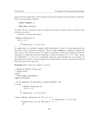
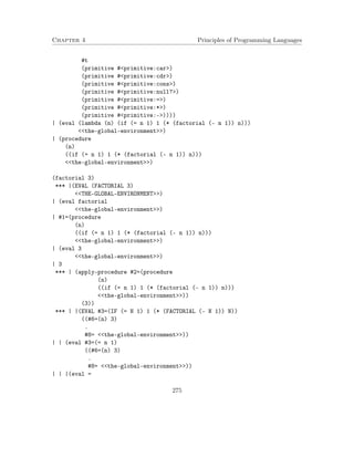
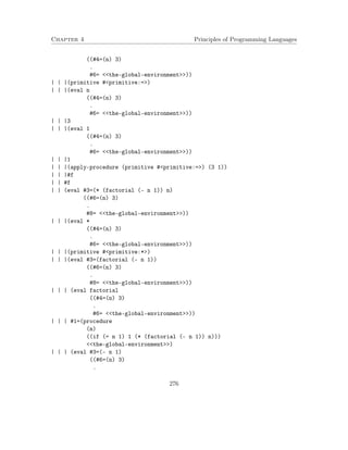
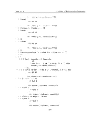
 2)
.
#6= the-global-environment))
| | | |[10](primitive #primitive:-)
| | | |[10](eval n
((#4=(n) 2)
278](https://image.slidesharecdn.com/principlesofprogramminglanguages-140901163422-phpapp01/85/Principles-of-programming-languages-283-320.jpg)
![Chapter 4 Principles of Programming Languages
.
#6= the-global-environment))
| | | |[10]2
| | | |[10](eval 1
((#4=(n) 2)
.
#6= the-global-environment))
| | | |[10]1
| | | |[10](apply-procedure (primitive #primitive:-) (2 1))
| | | |[10]1
| | | | | 1
*** | | | | | (apply #2=(procedure
(n)
((if (= n 1) 1 (* (factorial (- n 1)) n)))
the-global-environment))
(1))
*** | | | |[10](EVAL #3=(IF (= N 1) 1 (* (FACTORIAL (- N 1)) N))
((#6=(N) 1)
.
#8= THE-GLOBAL-ENVIRONMENT))
| | | |[11](eval #3=(= n 1)
((#6=(n) 1)
.
#8= the-global-environment))
| | | |[12](eval =
((#4=(n) 1)
.
#6= the-global-environment))
| | | |[12](primitive #primitive:=)
| | | |[12](eval n
((#4=(n) 1)
.
#6= the-global-environment))
| | | |[12]1
| | | |[12](eval 1
((#4=(n) 1)
.
#6= the-global-environment))
| | | |[12]1
| | | |[12](apply-procedure (primitive #primitive:=) (1 1))
| | | |[12]#t
279](https://image.slidesharecdn.com/principlesofprogramminglanguages-140901163422-phpapp01/85/Principles-of-programming-languages-284-320.jpg)
![Chapter 4 Principles of Programming Languages
| | | |[11]#t
| | | |[11](eval 1
((#4=(n) 1)
.
#6= the-global-environment))
| | | |[11]1
| | | |[10]1
| | | | | 1
| | | | |1
| | | | |(eval n
((#4=(n) 2)
.
#6= the-global-environment))
| | | | |2
| | | | |(apply-procedure (primitive #primitive:*) (1 2))
| | | | |2
| | | | 2
| | | |2
| | | 2
| | |2
| | |(eval n
((#4=(n) 3)
.
#6= the-global-environment))
| | |3
| | |(apply (primitive #primitive:*) (2 3))
| | |6
| | 6
| |6
| 6
|6
The body of the factorial procedure was analyzed 4 times. Assume now that we compute
(factorial 4)
24
The code of factorial body is again analyzed 5 times. The problem:
env-eval performs code analysis and evaluation simultaneously, which leads to
major inefficiency due to repeated analysis.
Evaluation tools distinguish between
280](https://image.slidesharecdn.com/principlesofprogramminglanguages-140901163422-phpapp01/85/Principles-of-programming-languages-285-320.jpg)
![Chapter 4 Principles of Programming Languages
turns into:
(define env-eval
(lambda (exp)
(lambda (env)
analyzed-body))
That is: analyze: Scheme-exp – Closure (env) ... The analyzer env-eval can
be viewed as a Curried version of env-eval.
Therefore, the derive-analyze-eval is defined by:
; Type: [Scheme-exp - [(Env - Scheme-type)]]
(define (derive-analyze-eval exp)
((analyze (derive exp)) the-global-environment))
where, the analysis of exp and every sub-expression of exp is performed only once, and
creates already compiled Scheme procedures. When run time input is supplied (the env
argument), these procedures are applied and evaluation is completed.
analyze is a compiler that performs partial evaluation of the env-eval computation.
We can even separate analysis from evaluation by saving the compiled code:
(define exp1 ’some-Scheme-expression)
(define compiled-exp1 (analyze (derive exp1)))
(compiled-exp1 the-global-environment)
Compiled-exp1 is a compiled program (a Scheme expression) that can be evaluated by
applying it to the-global-environment variable.
There are two principles for switching from env-eval code to a Curried analyze code.
1. Curry the env parameter.
2. Inductive application of analyze on all sub-expressions.
The Env-eval – analyzer transformation is explained separately for every kind of Scheme
expressions.
4.5.1.1 Atomic expressions:
In the env-eval:
(define eval-atomic
(lambda (exp env)
(if (or (number? exp) (boolean? exp) (null? exp))
exp
(lookup-variable-value env exp))))
282](https://image.slidesharecdn.com/principlesofprogramminglanguages-140901163422-phpapp01/85/Principles-of-programming-languages-287-320.jpg)
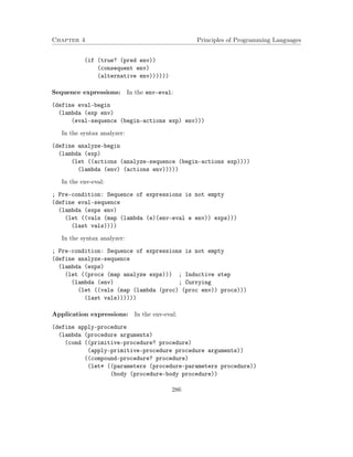
![Chapter 4 Principles of Programming Languages
(env (procedure-environment procedure))
(new-env (extend-env (make-frame parameters arguments) env)))
(eval-sequence body new-env)))
(else (error ’apply unknown procedure type: ~s procedure)))))
In the syntax analyzer:
(define analyze-application
(lambda (exp)
(let ((application-operator (analyze (operator exp)))
(application-operands (map analyze (operands exp))))
; Inductive step
(lambda (env)
(apply-procedure
(application-operator env)
(map (lambda (operand) (operand env))
application-operands))))))
The analysis of general application first extracts the operator and operands of the expres-sion
and analyzes them, resulting Curried Scheme procedures: Environment dependent exe-cution
procedures. At run time, these procedures are applied, resulting (hopefully) an eval-uator
procedure and its operands – Scheme values. These are passed to apply-procedure,
which is the equivalent of apply-procedure in env-eval.
; Type: [Analyzed-procedure*LIST - Scheme-type]
(define apply-procedure
(lambda (procedure arguments)
(cond ((primitive-procedure? procedure)
(apply-primitive-procedure procedure arguments))
((compound-procedure? procedure)
(let* ((parameters (procedure-parameters procedure))
(body (procedure-body procedure))
(env (procedure-environment procedure))
(new-env (extend-env (make-frame parameters arguments) env)))
(body new-env)))
(else (error ’apply unknown procedure type: ~s procedure)))))
If the procedure argument is a compound procedure of the analyzer, then its body is already
analyzed, i.e., it is an Env-Curried Scheme closure (of the target Scheme language) that
expects a single env argument.
Note: No recursive calls for further analysis; just direct application of the already analyzed
closure on the newly constructed extended environment.
287](https://image.slidesharecdn.com/principlesofprogramminglanguages-140901163422-phpapp01/85/Principles-of-programming-languages-292-320.jpg)
![Chapter 4 Principles of Programming Languages
4.5.1.3 Main analyzer loop:
Modifying the evaluation execution does not touch the two auxiliary packages:
Abstract Syntax Parser package.
Data Structures package.
The evaluator of the analyzed code just applies the result of the syntax analyzer:
(define derive-analyze-eval
(lambda (exp)
((analyze (derive exp)) the-global-environment)))
The main load is put on the syntax analyzer. It performs the case analysis, and dispatches
to procedures that perform analysis alone. All auxiliary analysis procedures return env
Curried execution Scheme closures.
; Type: [Scheme-exp - [(Env - Scheme-type)]]
; (Number, Boolean, Pair, List, Evaluator-procedure)
; Pre-conditions: The given expression is legal according to the concrete syntax.
; Inner ’define’ expressions are not legal.
(define analyze
(lambda (exp)
(cond ((atomic? exp) (analyze-atomic exp))
((special-form? exp) (analyze-special-form exp))
((application? exp) (analyze-application exp))
(else (error ’eval unknown expression type: ~s exp)))))
The full code of the analyzer is in the course site.
Example 4.14. (analyze 3) returns the Scheme closure: Closure (env) 3
(analyze 3)
#procedure ;;; A procedure of the underlying Scheme.
((analyze 3) the-global-environment)
3
Example 4.15.
(analyze ’car)
#procedure ;;; A procedure of the underlying scheme.
((analyze ’car) the-global-environment)
(primitive #primitive:car) ;;; An evaluator primitive procedure.
288](https://image.slidesharecdn.com/principlesofprogramminglanguages-140901163422-phpapp01/85/Principles-of-programming-languages-293-320.jpg)
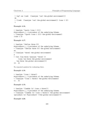
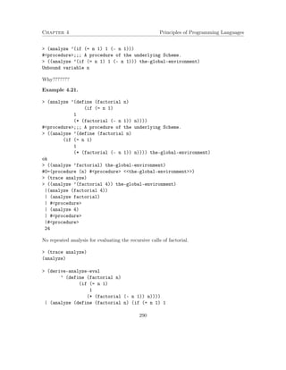
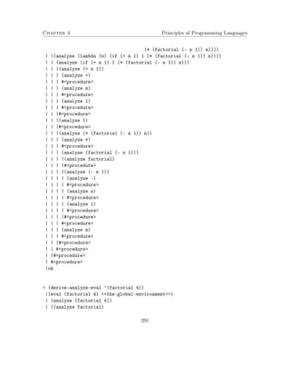
![Chapter 5
Logic Programming - in a Nutshell
Sources:
1. Sterling and Shapiro [11]: The Art of Prolog.
Topics:
1. Relational logic programming: Programs specify relations among entities.
2. Logic programming: Programs with data structures: Lists, binary trees, symbolic
expressions, natural numbers.
3. Meta tools: Backtracking optimization (cuts), unify, meta-circular interpreters.
4. Prolog and more advanced programming: Arithmetic, cuts, negation.
Introduction
The origin of Logic Programming is in constructive approaches in Automated Theorem
Proving, where logic proofs answer queries and construct instantiation to requested variables.
The idea behind logic programming suggests a switch in mode of thinking:
1. Structured logic formulas are viewed as relationship (procedure) specifications.
2. A query about logic implication is viewed as a relationship (procedure) call .
3. A constructive logic proof of a query is viewed as a query computation, dictated by
an operational semantics algorithm.
Logic programming, like functional languages (e.g., ML, Scheme), departs radically from
the mainstream of computer languages. Its operational semantics is not based on the Von-
Neumann machine model (like a Turing machine), but is derived from an abstract model
293](https://image.slidesharecdn.com/principlesofprogramminglanguages-140901163422-phpapp01/85/Principles-of-programming-languages-298-320.jpg)
![Chapter 5 Principles of Programming Languages
of constructive logic proofs (resolution proofs). In comparison, the operational semantics of
functional languages is based on the Lambda-calculus reduction rules.
In the early 70s, Kowalski [7] observed that an axiom:
A if B1 and B2 ... and Bn
can be read as a procedure of a recursive programming language:
A is the procedure head and the Bis are its body.
An attempt to solve A is understood as its execution: To solve (execute) A, solve
(execute) B1 and B2 ... and Bn.
The Prolog (Programming in Logic) language was developed by Colmerauer and his
group, as a theorem prover, embodying the above procedural interpretation.
Prolog has developed beyond the original logic basis. Therefore, there is a distinction
between (pure) logic programming to full Prolog. The Prolog language includes prac-tical
programming constructs, like primitives for arithmetics, and meta-programming and
optimization constructs, that are beyond the pure logic operational semantics.
A programming language has three fundamental aspects:
1. Syntax - concrete and abstract grammars, that define correct (symbolic) combina-tions.
2. Semantics - the things (values) computed by the programs of the language.
3. Operational semantics - an evaluation algorithm for computing the semantics of a
program.
For logic programs:
1. Syntax - a restricted subset of predicate calculus: A logic program is a set of formulas
(classified into rules and facts), defining known relationships in the problem domain.
2. Semantics - A set of answers to queries:
A program is applied to (or triggered by) a goal (query) logic statement. The
goal might include variables.
The semantics is a set of answers to goal queries. If a goal includes variables, the
answers provide substitutions (instantiations) for the variables in a query.
3. Operational semantics - Program execution is an attempt to prove a goal statement.
The proof tries to instantiate the variables (provide values for the variables),
such that the goal becomes true.
294](https://image.slidesharecdn.com/principlesofprogramminglanguages-140901163422-phpapp01/85/Principles-of-programming-languages-299-320.jpg)
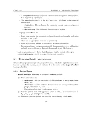
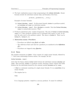
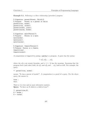
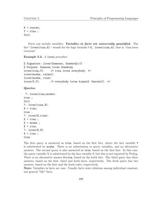
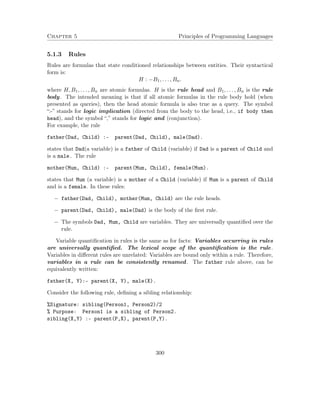
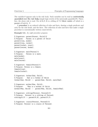
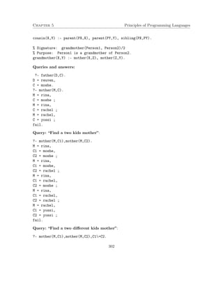
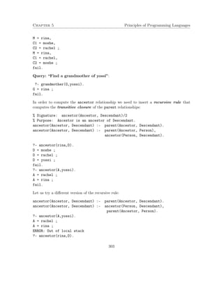
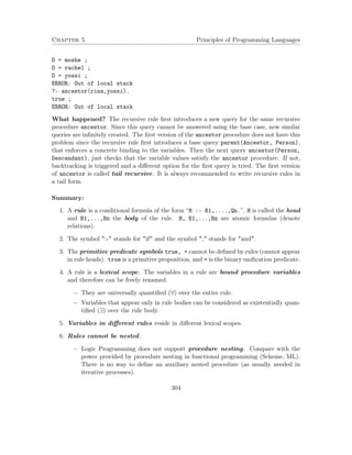
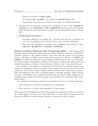
![Chapter 5 Principles of Programming Languages
A unification algorithm:
Signature: unify(A;B)
Type: [Atomic-formula*Atomic-formula - Substitution or FAIL]
Post-condition: result = mgu(A;B) if A and B are unifiable or FAIL, otherwise
unify(A,B) =
let help(s) =
if A s = B s then s
else let D = disagreement-set(A s, B s)
in if D = {X, t} /* X is a variable; t is a term
then help(s {X = t})
else FAIL
end
in help( {} )
end
Example 5.4.
1. unify[ p(X, 3, X, W), p(Y, Y, Z, Z) ] ==
help[ {} ] ==
D = {X, Y}
help[ {X = Y} ] ==
D = {Y, 3}
help[ {X = 3, Y= 3} ] ==
D = {Z, 3} ]
help[ {X = 3, Y= 3, Z = 3} ] ==
D = {W, 3}
help[ {X = 3, Y= 3, Z:= 3, W = 3} ] ==
{X = 3, Y = 3, Z = 3, W = 3}
2. unify[ p(X, 3, X, 5), p(Y, Y, Z, Z) ] ==
FAIL
Properties of this unification algorithm:
1. The algorithm terminates, because in every recursive call a variable is substituted, and
there is a finite number of variables.
2. The algorithm’s complexity is quadratic in the length of the input formulas (the exact
complexity depends on the implementation, whether it is incremental or not). In real
applications variables are not actually substituted. Instead, bindings are kept.
3. There are more efficient algorithms!
309](https://image.slidesharecdn.com/principlesofprogramminglanguages-140901163422-phpapp01/85/Principles-of-programming-languages-314-320.jpg)
![Chapter 5 Principles of Programming Languages
if label(current_node) is ?- true, ..., true.
then 1. Mark current_node as a Success node (leaf).
2. If the path from the tree root to current_node is labeled with the substitutions
s1; : : : ; sn, respectively, set_label!(current_node; s1 s2 : : : sn).
else 1. Select a goal G6= true in label(current_node) according to Gsel.
2. Rename variables in every rule and fact of P (justified since all variables are
universally quantified, i.e., bound).
3. While has-next?(iterator(current_node)):
(a) Advance iterator: next(iterator(current_node))
(b) Rule selection: Starting from iterator(current_node), and according to
Rsel, select a rule R = [A :- B1, ..., Bm.] such that unify(A;G) = s
succeeds with the unifying substitution (mgu) s.
(c) Rule application: (Reduce step)
if a rule R is selected
then
i. Construct a new query node by removing G, adding the body of
R, and applying s0 to the resulting query:
new_node = make_node([label(current_node)G+B1,...,Bm] s)
ii. Add a child node and start a new proof:
add_child(current_node; hs; number(R)i; new_node)
proof-tree(new_node)
Comments:
1. In the rename step, the variables in the rules are renamed by new names. This way
the program variables in every binding step are different from previous steps. Since
variables in rules are bound procedure variables they can be freely renamed.
Renaming convention: In every recursive call, increase some auxiliary counter, such
that variables X, Y,... are renamed as X1, Y1,... at the first level, X2, Y2,... at
the second level, etc.
2. Advice for substitution in the rule selection step: Let unify produce a substitution to
the rule head variables, rather than to the goal variables. This way the query variables
are kept in the substitutions produced in a proof branch. Since the mgu is unique up
to renaming, the proof is indifferent to whether it includes varrule_head := vargoal or
vargoal := varrule_head.
3. The goal and rule selection decisions can affect the performance of the interpreter.
313](https://image.slidesharecdn.com/principlesofprogramminglanguages-140901163422-phpapp01/85/Principles-of-programming-languages-318-320.jpg)
![Chapter 5 Principles of Programming Languages
The answer-query algorithm – the virtual version:
Input:
A query: Q = ?- Q1, ..., Qn.
A program P
A goal selection rule Gsel
A rule selection rule Rsel
Output:
A set of substitutions for variables of Q (not necessarily for all variables).
Method:
1. answer = answer-query-help(Q; P; fg;new iterator(); fg)
2. return: answer, restricted to the variables in Q.
The answer-query-help algorithm:
Input:
A query: Q = ?- Q1, ..., Qn.
A program P
A substitution s
A rule iterator it
A set of answer substitutions subs
Output: A set of substitutions.
Method:
answer-query-help(Q; P; s; it; subs) =
1. If Q = ?- true, ..., true.: Return subs [ fsg.
2. Select a goal G6= true in Q according to Gsel.
3. Rename variables in every rule and fact of the program P.
4. Rule selection: Starting from it, and according to Rsel, select a rule R = [A
:- B1, ..., Bm.] such that unify(A;G) = s0, the unifying substitution.
5. Rule application: If a rule R is selected
(a) Construct a new query Q0 by removing G, adding the body of R, and
applying s0 to the resulting query:
Q0 = [Q G+ B1,...,Bm ] s0
(b) Prove the new query, under the new substitution, and a new iterator:
new_subs = answer-query-help(Q0; P; s s0; new iterator(); subs)
314](https://image.slidesharecdn.com/principlesofprogramminglanguages-140901163422-phpapp01/85/Principles-of-programming-languages-319-320.jpg)
![Chapter 5 Principles of Programming Languages
Figure 5.1: The proof tree - a finite success tree
Definition: [Provable query]
A query Q is provable from a program P, denoted P ` Q, iff for some goal and rule
selection rules Gsel and Rsel, the proof tree algorithm for answer-query(Q; P; Gsel;Rsel)
computes a success tree.
A finite root-to-leaf path with a non Success marked leaf is a finite-failure com-putation
path. A proof tree that all of its paths are failed computation paths is a
(finite) failure tree.
An infinite computation path is an infinite path. Infinite computations can be
created by recursive rules (direct or indirect recursion).
Significant kinds of proof trees:
1. Finite success proof tree: A finite tree with a successful path.
2. (Finite) Failure proof tree: A finite tree with no successful path.
3. Infinite success proof tree: An infinite tree with a successful path. In this case it
is important not to explore an infinite path. For Prolog: Tail recursion is safe, while
left recursion is dangerous.
4. Infinite failure proof tree: An infinite tree with no successful path. Dangerous to
explore.
316](https://image.slidesharecdn.com/principlesofprogramminglanguages-140901163422-phpapp01/85/Principles-of-programming-languages-321-320.jpg)
![Chapter 5 Principles of Programming Languages
The proof tree in Example 5.5 is a finite success tree. The resulting substitution on
the successful computation path is: {X1=S, Y1=haran} {S=lot}, which is the substitu-tion
{X1=lot, Y1=haran, S=lot}. The restriction to the query variables yields the single
substitution: {S=lot}.
Properties of answer-query:
1. Proof tree uniqueness: The proof tree for a given query and a given program is
unique, for all goal and rule selection procedures (up to sibling ordering).
Conclusion: The set of answers is independent of the concrete selection procedures
for goals and rules.
2. Performance: Goal and rule selection decisions have impact on performance.
(a) The rules of a procedure should be ordered according to the rule selection pro-cedure.
Otherwise, the computation might get stuck in an infinite path, or try
multiple failed computation paths.
(b) The atomic formulas in a rule body should be ordered according to the goal
selection procedure.
3. Soundness and completeness:
Definition: [logical implication]
A query Q is logically implied from a program P, denoted P j= Q, if it is true
whenever the program is true.
Completeness: P j= Q implies P ` Q. That is, if a query is logically implied
from a program, then it is also provable by answer-query.
Soundness: P ` Q implies P j= Q. That is, if a query is provable by answer-query,
then it is logically implied from the program.
5.1.5.3 Properties of Relational Logic Programming
Decidability:
Proposition 5.1.1. Given a program P and a query Q, the problem Is Q provable from
P, denoted P ` Q, is decidable.
Proof. The proof tree consists of nodes that are labeled by queries, i.e., sequences of atomic
formulas. The atomic formulas consist of predicate and individual constant symbols that
occur in the program and the query, and from variables. Therefore, (1) the number of atomic
formulas is finite, up to variable renaming, and (2) the number of different selected goals in
queries on a path is finite (up to variable renaming). Consequently, every path in the proof
tree can be decided to be a success, a failure or an infinite computation path.
317](https://image.slidesharecdn.com/principlesofprogramminglanguages-140901163422-phpapp01/85/Principles-of-programming-languages-322-320.jpg)
![Chapter 5 Principles of Programming Languages
cons(a,[ ]) – describes the list [a]. [ ] is an individual constant, standing for the
empty list. The cons functor has a syntactic sugar notation as an infix operator |:
cons(a,[ ]) is written: [a|[ ]].
cons(b,cons(a,[ ])) – the list [b,a], or [b|[a|[ ]]]. The syntax [b,a] uses the
printed form of lists in Prolog.
cons(cons(a,[ ]), cons(b,cons(a,[ ]))) – the list [[a],[b,a]], or [[a|[ ]]|[b|[a,|[
]]]].
time(monday,12,14)
street(alon,32)
tree(Element,Left,Right) – a binary tree, with Element as the root, and Left and
Right as its sub-trees.
tree(5,tree(8,void,void),tree(9,void,tree(3,void,void)))
Atomic formulas: The arguments to the predicate symbols in an atomic formula are terms:
father(abraham,isaac)
p(f(f(f(g(a,g(b,c))))))
ancestor(mary,sister_of(friend_of(john)))
append(cons(a,cons(b,[ ])),cons(c,cons(d,[ ])))
cons(a,cons(b,cons(c,cons(d,[ ]))))
append([a,b],[c,d],[a,b,c,d])
Notes:
1. Every functor has an arity: Number of arguments. In Example 5.6:
The arity of cons is 2.
The arity of sister_of is 1.
The arity of time is 3.
The arity of street is 2.
2. Functors can be nested: Terms might have unbound depth: f(f(f(g(a,g(b,c))))).
Therefore: The number of different atomic formulas that can be constructed from
a given set of predicate, functor and individual constant symbols is unbounded - in
contrast to the situation in Relational Logic Programming!
320](https://image.slidesharecdn.com/principlesofprogramminglanguages-140901163422-phpapp01/85/Principles-of-programming-languages-325-320.jpg)
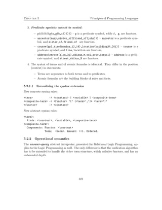
![Chapter 5 Principles of Programming Languages
5.2.2.1 Unification for terms that include functors (composite terms)
The presence of function symbols complicates the unification step in the abstract interpreter.
Recall that the rule selection procedure tries to unify a query goal (an atomic formula) with
the head of the selected rule (an atomic formula). The unification operation, if successful,
produces a substitution (most general unifier) for the variables in the atomic formulas.
The notion of substitution is modified as follows:
Definition: A substitution s is a finite mapping from variables to terms, such that s(X)
does not include X.
All other substitution and unification terminology stays unchanged.
unify(member(X,tree(X,Left,Right)) ,
member(Y,tree(9,void,tree(3,void,void))))
yields the mgu substitution: {Y:=9, X:=9, Left:=void, Right=tree(3,void,void)}
unify(member(X, tree(9,void,tree(E1,L1,R1)) ,
member(Y,tree(Y,Z,tree(3,void,void))))
yields the mgu substitution: {Y:=9, X:=9, Z:=void, E1:=3, L1:=void, R1:=void}
unify(t(X,f(a),X),t(g(U),U,W))
yields the mgu substitution: {X:=g(f(a)), U:=f(a), W:=g(f(a))}
unify(t(X,f(X),X),t(g(U),U,W))
fails!
unify(append([1,2,3],[3,4],List),
append([X|Xs],Ys,[X|Zs]))
yields the mgu substitution: {X:=1, Xs:=[2,3], Ys:=[3,4], List:=[1|Zs]}
unify(append([1,2,3],[3,4],[3,3,4]),
append([X|Xs],Ys,[Xs|Zs]))
fails!
322](https://image.slidesharecdn.com/principlesofprogramminglanguages-140901163422-phpapp01/85/Principles-of-programming-languages-327-320.jpg)
![Chapter 5 Principles of Programming Languages
The unification algorithm presented for Relational Logic Programming applies also to
Logic Programming. The only difference appears in the kind of terms that populate the
disagreement sets that are computed, and an occur check restriction that prevents
infinite unification efforts.
1. Disagreement sets:
disagreement-set(t(X; f(a);X);
t(g(U);U;W)) = fX; g(U)g
disagreement-set(append([1; 2; 3]; [3; 4]; List);
append([1jXs]; Y s; [XjZs])) = f[2; 3];Xsg
disagreement-set(append([1; 2; 3]; [3; 4]; [3; 3; 4]);
append([1; 2; 3]; [3; 4]; [[1; 2]jZs])) = f3; [1; 2]g
2. Occur check:
disagreement-set(t(g(U); f(g(U)); g(U));
t(g(U);U;W)) = ff(g(U));Ug
The disagreement set in the unify algorithm is used for constructing the mgu sub-stitution,
in case that one of its components is a variable. Otherwise, the unification
fails. But in case that the disagreement set includes a binding hX; s(X)i, such that
s(X) includes X as in the above example, the mgu cannot be constructed, and the
unification fails.
Therefore, the unification algorithm is extended with the occur check constraint.
A unification algorithm:
Signature: unify(A,B)
Type: [Atomic-formula*Atomic-formula - Substitution union FAIL]
Post-condition: result = mgu(A,B) if A and B are unifiable
or FAIL, otherwise
unify(A,B) =
let help(s) =
if A s = B s then s
else let D = disagreement-set(A s, B s)
in if [D = {X, t} and X does not occur in t]
/* The occur check constraint
then help(s {X = t})
else FAIL
end
in help( {} )
end
323](https://image.slidesharecdn.com/principlesofprogramminglanguages-140901163422-phpapp01/85/Principles-of-programming-languages-328-320.jpg)
![Chapter 5 Principles of Programming Languages
Comparison of the logic programming unification with the ML pattern matching:
1. In ML patterns appear only in function definitions. Expressions in function calls are
first evaluated, and do not include variables when matched.
2. Patterns in ML do not allow repeated variables. Compare:
Logic programming ML
append([], Xs, XS). val rec append =
append([X|Xs], Ys, [X|Zs] :- fn ( [],lst ) = lst
append(X, Ys, Zs). | (h::tail, lst) =
h::append(tail,lst)
member(X, [X|Xs). val rec member =
member(X, [Y|Ys]) :- fn (el, []) = false
member(X, Ys). | (el, [h::tail] =
el = h orelse member(el,tail)
3. ML restricts pattern matching to equality types. In logic programming, since there
is no evaluation, and comparison is by unification rather than equality, there are no
restrictions.
Expressivity and decidability of Logic Programming:
1. Logic Programming has the expressive power of Turing machines. That is, every com-putable
program can be written in Logic Programming. In particular, every Scheme
or ML program can be written in Prolog, and vice versa.
2. Logic Programming is only partially decidable - unlike Relational Logic Programming.
That is, the problem Is Q provable from P, denoted P |- Q, is partially decidable.
The finiteness argument of Relational Logic Programming does not apply here since
in presence of functors, the number of different atomic formulas is unbounded (since
terms can be nested up to unbounded depth). Therefore, terminating proofs can have
an unbounded length.
5.2.3 Data Structures
5.2.3.1 Trees
1. Defining a tree
324](https://image.slidesharecdn.com/principlesofprogramminglanguages-140901163422-phpapp01/85/Principles-of-programming-languages-329-320.jpg)
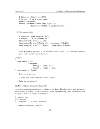
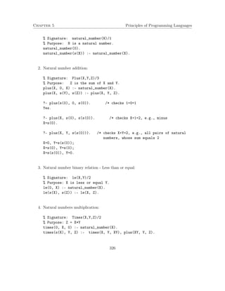
![Chapter 5 Principles of Programming Languages
5.2.3.3 Lists
1. Syntax:
[ ] is the empty list.
[Head|Tail] is a syntactic sugar for cons(Head, Tail), where Tail is a list term.
Simple syntax for bounded length lists:
[a|[ ]] = [a]
[a|[ b|[ ]]] = [a,b]
[rina]
[sister_of(rina),moshe|[yossi,reuven]] = [sister_of(rina),moshe,yossi,reuven]
Defining a list:
list([]). /* defines the basis
list([X|Xs]) :- list(Xs). /* defines the recursion
2. List membership:
% Signature: member(X, List)/2
% Purpose: X is a member of List.
member(X, [X|Xs]).
member(X, [Y|Ys]) :- member(X, Ys).
?- member(a, [b,c,a,d]). /* checks membership
?- member(X, [b,c,a,d]). /* takes an element from a list
?- member(b, Z). /* generates a list containing b
3. List concatenation:
% Signature: append(List1, List2, List3)/3
% Purpose: List3 is the concatenation of List1 and List2.
append([], Xs, Xs).
append([X|Xs], Y, [X|Zs] ) :- append(Xs, Y, Zs).
?- append([a,b], [c], X). /* addition of two lists
?- append(Xs, [a,d], [b,c,a,d]). /* finds a difference between lists
?- append(Xs, Ys, [a,b,c,d]). /* divides a list into two lists
4. List selection using append:
327](https://image.slidesharecdn.com/principlesofprogramminglanguages-140901163422-phpapp01/85/Principles-of-programming-languages-332-320.jpg)
![Chapter 5 Principles of Programming Languages
(a) List prefix and suffix:
prefix(Xs, Ys) :- append(Xs, Zs, Ys).
suffix(Xs, Ys) :- append(Zs, Xs, Ys).
Compare the power of this one step unification with the equivalent Scheme code,
that requires climbing the list until the prefix is found, and guessing the
suffix.
(b) Redefine member:
member(X, Ys) :- append(Zs, [X|Xs], Ys).
(c) Adjacent list elements:
adjacent(X, Y, Zs) :- append(Ws, [X,Y|Ys], Zs).
(d) Last element of a list:
last(X, Ys) :- append(Xs, [X], Ys).
5. List Reverse:
(a) A recursive version:
% Signature: reverse(List1, List2)/2
% Purpose: List2 is the reverse of List1.
reverse([], []).
reverse([H|T], R) :- reverse(T, S), append(S, [H], R).
?- reverse([a,b,c,d],R).
R=[d,c,b,a]
But, what about:
?- reverse(R,[a,b,c,d]).
Starting to build the proof tree, we see that the second query is
?- reverse(T1,S1), append(S1, [H1], [a,b,c,d]).
This query fails on the first rule, and needs the second. The second rule is applied
four times, until four elements are unified with the four elements of the input list.
We can try reversing the rule body:
328](https://image.slidesharecdn.com/principlesofprogramminglanguages-140901163422-phpapp01/85/Principles-of-programming-languages-333-320.jpg)
![Chapter 5 Principles of Programming Languages
reverse([H|T], R) :- append(S, [H], R), reverse(T, S).
The new version gives a good performance on the last direction, but poor perfor-mance
on the former direction.
Conclusion: Rule body ordering impacts the performance in various directions.
What about reversing rule ordering? In the reversed direction - an infinite
loop.
Typical error: Wrong assembly of resulting lists:
wrong_reverse([H|T], R):-
wrong_reverse(T, S), append(S, H, R).
(b) An iterative version:
% Signature: reverse(List1, List2)/2
% Purpose: List2 is the reverse of List1. This version uses an additional
reverse helper procedure, that uses an accumulator.
reverse(Xs, Ys):- reverse_help(Xs,[],Ys).
reverse_help([X|Xs], Acc, Ys ) :-
Reverse_help(Xs,[X|Acc],Ys).
reverse_help([ ],Ys,Ys ).
?- reverse([a,b,c,d],R).
R=[d,c,b,a]
The length of the single success path is linear in the list length, while in the
former version it is quadratic.
Note: The reverse_help procedure is an helper procedure that should not reside
in the global name space. Unfortunately, Logic Programming does not support
nesting of name spaces (like Scheme, ML, Java). All names reside in the
global space.
Summary of Logic Programming:
1. Identical syntax to terms and atomic formulas. Distinction is made by syntactical
context (recall, in analogy, the uniform syntax of Scheme composite expressions and
Scheme lists).
2. No language primitives - besides true, =.
3. No computation direction: Procedures (predicates) define relations, not functions.
329](https://image.slidesharecdn.com/principlesofprogramminglanguages-140901163422-phpapp01/85/Principles-of-programming-languages-334-320.jpg)
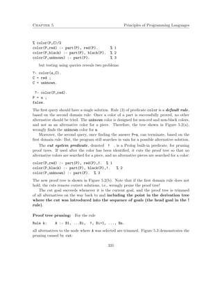
![Chapter 5 Principles of Programming Languages
Example 5.8. Erroneous alternatives: Consider the following erroneous program that in-tends
to check whether every list element of a list includes some key:
% Signature: badAllListsHave(List,Key)/2
% Purpose: Check whether Key is a member of every element of List
% which is a list.
% Type: List is a list.
badAllListsHave( [First|Rest],Key):-
is_list(First), member(Key,First),badAllListsHave( Rest,Key).
badAllListsHave( [_|Rest],Key):- badAllListsHave( Rest,Key).
badAllListsHave( [ ],_).
The query
?- badAllListsHave( [ [2], [3] ],3).
succeeds, since the second rule enables skipping the first element of the list. The point is
that once the is_list(First) goal in the first rule succeeds, the second rule cannot function
as an alternative. Inserting a cut after the is_list(First) goal solves the problem, since
it prunes the erroneous alternative from the tree:
% Signature: allListsHave(List,Key)/2
% Purpose: Check whether Key is a member of every element of List
% which is a list.
% Type: List is a list.
allListsHave( [First|Rest],Key):-
is_list(First), !, member(Key,First),allListsHave( Rest,Key).
allListsHave( [_|Rest],Key):-
badAllListsHave( Rest,Key).
allListsHave( [ ],_).
Example 5.9. Exclusive rules (using arithmetics):
% Signature: minimum(X,Y,Min)/3
% Purpose: Min is the minimum of the numbers X and Y.
% Type: X,Y are Numbers.
% Pre-condition: X and Y are instantiated.
minimum(X,Y,X) :- X = Y,!.
minimum(X,Y,Y) :- XY.
The cut prevents useless scanning of the proof tree.
But:
333](https://image.slidesharecdn.com/principlesofprogramminglanguages-140901163422-phpapp01/85/Principles-of-programming-languages-338-320.jpg)
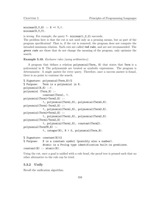
![Chapter 5 Principles of Programming Languages
Signature: unify(A,B)
Type: [Atomic-formula*Atomic-formula - Substitution union FAIL]
Post-condition: result = mgu(A,B) if A and B are unifiable
or FAIL, otherwise
unify(A,B) =
let help(s) =
if A s = B s then s
else let D = disagreement-set(A s, B s)
in if [D = {X, t} and X does not occur in t]
/* The occur check constraint
then help(s {X = t})
else FAIL
end
in help( {} )
end
The algorithm can be implemented in Logic Programming, but it requires some extra log-ical
tools for inspection of term structure. The algorithm is based on the apply-substitution
operation, and requires the ability to
1. Distinguish between different variables.
2. Distinguish between variables to constants.
The implementation below assumes that the given atomic formulas have been pre-processed
into ground terms (not including variables), such that constants denoting vari-ables
are distinguished from true constants. For example, the atomic formulas c(f(X), G,
X), c(G, Y, f(d)) turn into: c(f(x), g, x), c(g, y, f(d)). The implementation uses
the meta-programming predicate univ, denoted =.., which turns a term into a list of the
functor followed by the arguments. For example:
1 ?- f(a,X,g(Y))=..Term_list.
Term_list = [f, a, X, g(Y)].
2 ?- Term=..[f, a, X, g(Y)].
Term = f(a, X, g(Y)).
The distinction between variables to constants is implemented using a variable and a constant
predicates.
We present first the substitute procedure, which implements the apply-substitution
operation.
% Signature: substitute(Exp, S, ExpS)/3
% Purpose: ExpS is the application of a substitution S on a ground term Exp.
% Examples:
335](https://image.slidesharecdn.com/principlesofprogramminglanguages-140901163422-phpapp01/85/Principles-of-programming-languages-340-320.jpg)
![Chapter 5 Principles of Programming Languages
% constant_list([ a, b, c, d, [], 5, 6]).
% variable_list([x, y, z]).
% ?- substitute(p(a, b(x), c(d(y)), x), [[z, 5], [x, 6]], Ans).
% Ans = p(a, b(6), c(d(y)), 6).
% Pre-condition: All logic programming constant symbols in a query must be
% declared either as expression constants or as expression
% variables. That is, belong to one of the constant or variable
% lists. Otherwise, the program enters an infinite loop.
%
substitute(Exp, [], Exp) :- !. %1
% green cut to avoid backtracking in (2)-(6)
substitute(X, S, XS) :- variable(X), member([X, XS], S), %2
!. % red cut to avoid backtracking in (3)
substitute(X, S, X) :- variable(X), %3
!. % green cut to avoid univ of atom in (6)
substitute(X, S, X) :- constant(X), %4
!. % green cut to avoid univ of atom in (6)
substitute([E|Exp],S,[ES|ExpS]) :- %5
!, % red cut to avoid [E|Exp] unification in (6)
substitute(E, S, ES), substitute(Exp, S, ExpS),
!. % green cut to avoid rerun of the code
substitute(Exp, S, ExpS) :- Exp =.. List, %6
substitute(List, S, ListS), ExpS =.. ListS.
unify is a three-ary predicate, with two parameters that are the terms to be unified, and a
third ‘mgu parameter.
% Signature: unify(A, B, Mgu)/3
% Examples:
% ?- unify(a(x, 5), a(6, y), Mgu).
% Mgu = [[y, 5], [x, 6]].
% ?- unify(c(a(x), z, x), c(z, y, a(d)), Mgu).
% Mgu = [[x, a(d)], [y, a(a(d))], [z, a(a(d))]]
% ?- unify(c(a(x), d, x), c(z, y, a(z)), Mgu).
% false
%
unify(A, B, Mgu) :- help(A, B, [], Mgu). %1
help(A, B, S, Mgu) :- substitute(A, S, AS), %1
substitute(B, S, BS),
help_helper(A, B, S, AS, BS, Mgu).
336](https://image.slidesharecdn.com/principlesofprogramminglanguages-140901163422-phpapp01/85/Principles-of-programming-languages-341-320.jpg)
![Chapter 5 Principles of Programming Languages
help_helper(A, B, S, AS, AS, S) :- !. %2
% green cut to avoid disagreement run in (3)
help_helper(A, B, S, AS, BS, Mgu) :- disagreement(AS, BS, [X, T]), %3
not_occurs(T, X),
substitute(S, [[X, T]], SS),
help(A, B, [[X, T]|SS], Mgu).
The disagreement and the not_occur procedures:
% Signature: disagreement(A, B, Set)/3
disagreement(AS, BS, [AS, BS]) :- variable(AS), %1
% green cut to avoid backtracking in (5)
disagreement(AS, BS, [BS, AS]) :- variable(BS), %2
!. % green cut to avoid backtracking in (6)
disagreement([A|AS], [A|BS], [X, T]) :- !, %3 red cut to avoid backtracking in (7)
disagreement(AS, BS, [X, T]).
disagreement([A|_], [B|_], [X, T]) :- !, %4 red cut to avoid backtracking in (7)
disagreement(A, B, [X, T]).
disagreement(AS, _, _) :- constant(AS), %5
!, % red cut to avoid univ of constant in (7)
fail.
disagreement(_, BS, _) :- constant(BS), %6
!, % red cut to avoid univ of constant in (7)
fail.
disagreement(A, B, [X, T]) :- A =.. A_list, %7
B =.. B_list,
disagreement(A_list, B_list, [X, T]).
% Signature: not_occurs(T, X)/2
%
not_occurs(X, X) :- !, %1 red cut to avoid backtracking in (2)
fail.
not_occurs(T, _X) :- variable(T), %2
!. % green cut to avoid univ of atom in (5)
not_occurs(T, _X) :- constant(T), %3
!. % green cut to avoid univ of atom in (5)
not_occurs([T|TT], X) :- !, %4 red cut to avoid univ of list in (5)
not_occurs(T, X), not_occurs(TT, X),
!. % green cut to avoid rerun of the code
not_occurs(T, X) :- T =.. T_list, %5
not_occurs(T_list, X).
337](https://image.slidesharecdn.com/principlesofprogramminglanguages-140901163422-phpapp01/85/Principles-of-programming-languages-342-320.jpg)
![Chapter 5 Principles of Programming Languages
% Signature: variable(Name)/1
variable(X) :- variable_list(Vars), member(X,Vars).
variable_list([x,y,z]).
% Signature: constant(Name)/1
constant(C) :- constant_list(Consts), member(C, Consts).
constant_list([p,a,b,c,d,[],5,6]).
5.3.3 Meta-circular interpreters for Logic Programming
Recall the abstract interpreter for logic programs.
1. It is based on unification, search, and backtracking.
(a) Goal selection - left most for Prolog.
(b) Rule selection - first for Prolog, with backtracking to the following rules, in case
of a failure.
2. It has two points of non-deterministic selection.
This behavior can be encoded into a logic programming procedure solve that implements
the abstract interpreter algorithm.
We present several solve procedures. The interpreters exploit the uniformity of the
syntax of terms and of atomic formulas: The atomic formulas of the program are read as
terms, for the interpreter1. All interpreters work in two stages:
1. Pre-processing: The given program P (facts and rules) is translated into a new
program P’, with a single predicate rule, with facts alone.
2. Queries are presented to the procedure solve, and to the transformed program P’.
The first interpreter is a “vanilla” one: A basic interpreter that fully uses Prolog’s rule and
goal selection rules. The rest of the interpreters vary either in providing also a proof tree in
addition to the proof, or in the amount of control they provide to goal selection order.
Pre-processing – Program transformation: The rules and facts of the logic program
are transformed into an all facts procedure rule. The rule:
A :- B1, B2, ..., Bn
Is transformed into the fact:
1Recall the Scheme meta-circular interpreter, which exploits the uniform syntax of Scheme expressions
and the printed form of lists.
338](https://image.slidesharecdn.com/principlesofprogramminglanguages-140901163422-phpapp01/85/Principles-of-programming-languages-343-320.jpg)
![Chapter 5 Principles of Programming Languages
rule(A, [B1, B2, ..., Bn] ).
A fact A. is transformed into rule(A, true). For example, the program:
% father(abraham, isaac).
% father(haran, lot).
% father(haran, milcah).
% father(haran, yiscah).
% male(isaac).
% male(lot).
% female(milcah).
% female(yiscah).
% son(X, Y) :- father(Y, X),
% male(X).
% daughter(X, Y) :- father(Y, X),
% female(X).
is transformed into the program:
rule(father(abraham, isaac), true). %1
rule(father(haran, lot), true). %2
rule(father(haran, milcah), true). %3
rule(father(haran, yiscah), true). %4
rule(male(isaac), true). %5
rule(male(lot), true). %6
rule(female(milcah), true). %7
rule(female(yiscah), true). %8
rule(son(X, Y), [father(Y, X), male(X)]). %9
rule(daughter(X, Y), [father(Y, X), female(X)]). %10
The new program consists of facts alone.
Vanilla (basic) interpreter
The vanilla interpreter simulates Prolog’s goal selection rule, and relies on Prolog’s rule
selection.
% Signature: solve(Exp)/1
% Purpose: Vanilla interpreter.
% Examples:
% ?- solve(son(lot, haran)).
% true.
%
% ?- solve(son(X, Y)).
339](https://image.slidesharecdn.com/principlesofprogramminglanguages-140901163422-phpapp01/85/Principles-of-programming-languages-344-320.jpg)
![Chapter 5 Principles of Programming Languages
% X = isaac,
% Y = abraham ;
% X = lot,
% Y = haran ;
% false.
%
solve(true). %1
solve([]). %2
solve([A|B]) :- solve(A), solve(B). %3
solve(A) :- rule(A,B), solve(B). %4
Interpreter operation: The first fact ends a proof of a fact, the second fact ends the proof
of a list of goals (the body of a program rule), the third rule selects a goal to prove, and the
fourth rule finds a program rule whose head unifies with the given goal. This interpreter
relies on Prolog for doing almost everything:
1. Reading and parsing the input.
2. Unification and rule selection (following the order of the rule procedure).
3. Goal selection and recursive computation (reduction).
Interpreter with associated proofs for answers:
Successful computations can be associated with a parse tree of the proof:
% Signature: solve(Exp, -Proof)/2
% Purpose: Interpreter and associate proofs with success answers
% Examples:
% ?- solve(son(lot,haran), Proof).
% Proof = node(son(lot,haran),
% [node(father(haran,lot),true),node(male(lot),true)]);
% false.
% ?- solve(son(X,Y), Proof).
% X = isaac,
% Y = abraham,
% Proof = node(son(isaac,abraham),
% [node(father(abraham,isaac),true),node(male(isaac),true)]) ;
% X = lot,
% Y = haran,
% Proof = node(son(lot,haran),
% [node(father(haran,lot),true),node(male(lot),true)]) ;
% false.
340](https://image.slidesharecdn.com/principlesofprogramminglanguages-140901163422-phpapp01/85/Principles-of-programming-languages-345-320.jpg)
![Chapter 5 Principles of Programming Languages
%
solve(true, true). %1
solve([], []). %2
solve([A|B],[ProofA|ProofB]) :- solve(A,ProofA), solve(B, ProofB). %3
solve(A, node(A,Proof)) :- rule(A,B), solve(B,Proof). %4
Interpreter operation:
1. The first two facts provide proofs to true and to the end of a proof.
2. The third rule structures the proof of list of goals as a list of proofs.
3. The fourth rule specifies the proof of an atomic goal A that unifies with the head of a
program rule with body B, to be a tree-node labeled by the goal A, and with the proof
of B as child trees.
To further clarify, given the propositional program
a :- b,c,d,e. %1
b :- f,g. %2
c. %3
d. %4
c. %5
e. %6
f. %7
g. %8
whose pre-processing yields:
rule(a, [b,c,d,e]). %1
rule(b, [f,g]). %2
rule(c, true). %3
rule(d, true). %4
rule(c, true). %5
rule(e, true). %6
rule(f, true). %7
rule(g, true). %8
6 ?- solve(a, Proof).
Proof = node(a, [node(b, [node(f, true), node(g, true)]),
% node(c, true),
% node(d, true),
% node(e, true)]) ;
Proof = node(a, [node(b, [node(f, true), node(g, true)]),
341](https://image.slidesharecdn.com/principlesofprogramminglanguages-140901163422-phpapp01/85/Principles-of-programming-languages-346-320.jpg)
![Chapter 5 Principles of Programming Languages
% node(c, true),
% node(d, true),
% node(e, true)]) ;
false.
Addition of failed proofs: Finite failure proofs can be added by detecting goals that
could not be computed by the former solve, and adding them as a failure node to the proof.
This can done by addition of two default rules at the end of the solve. One rule, number
5, eliminates failed goals that unify with some rule facts, and the last one, number 6, adds
the failure node.
% Signature: solve(Exp, Proof)/1
% Purpose: Interpreter and associate proofs with success answers.
% Examples:
% ?- solve(son(lot, haran), Proof).
% Proof = node(son(lot, haran),
% [node(father(haran, lot), true), node(male(lot), true)]);
% false.
% ?- solve(son(X, Y), Proof).
% X = isaac,
% Y = abraham,
% Proof = node(son(isaac, abraham),
% [node(father(abraham, isaac), true), node(male(isaac), true)]) ;
% X = lot,
% Y = haran,
% Proof = node(son(lot, haran),
% [node(father(haran, lot), true), node(male(lot), true)]) ;
% X = milcah,
% Y = haran,
% P = node(son(milcah, haran),
% [node(father(haran, milcah), true), node(male(milcah), fail)]) ;
% X = yiscah,
% Y = haran,
% P = node(son(yiscah, haran),
% [node(father(haran, yiscah), true), node(male(yiscah), fail)]) ;
% false.
%
solve(true, true) :- !. %1 red cut to avoid Proof unification in (6)
solve([], []) :- !. %2 red cut to avoid Proof unification in (6)
solve([A|B], [ProofA|ProofB]) :- !, %3 red cut to avoid Proof unification in (6)
solve(A, ProofA), solve(B, ProofB).
342](https://image.slidesharecdn.com/principlesofprogramminglanguages-140901163422-phpapp01/85/Principles-of-programming-languages-347-320.jpg)
![Chapter 5 Principles of Programming Languages
solve(A, node(A, Proof)) :- rule(A, B), solve(B, Proof). %4
solve(A, _) :- rule(A, _), %5
!, % red cut to avoid backtracking in (7)
fail.
solve(A, node(A, fail)). %6
Interpreter with management of goals
This interpreter uses an explicit control of the goal selection order, using a waiting list of
goals (reminds the CPS approach).
% Signature: solve(Exp)/1
% Purpose: Interpreter with explicit management of a waiting list of goals.
% Examples:
% ?- solve(son(lot, haran)).
% true.
% ?- solve(son(X, Y)).
% X = isaac,
% Y = abraham ;
% X = lot,
% Y = haran ;
% false.
%
solve(Goal) :- solve(Goal, []). %1
solve(true, Goals) :- solve([], Goals). %1
solve([], []). %2
solve([], [G|Goals]) :- solve(G, Goals). %3
solve([A|B], Goals) :- extend_waiting_list([A|B], Goals, NewGoals), %4
solve([], NewGoals).
solve(A, Goals) :- rule(A, B), solve(B, Goals). %5
% Signature: extend_waiting_list(Goals, WaitingList, NewWaitingList)/3
% Purpose: Extend the waiting list of goals.
%
extend_waiting_list(Goals, WaitingList, NewWaitingList) :- %1
% append(Goals, WaitingList, NewWaitingList).
Interpreter operation: The interpreter solve/2 keeps the goals to be proved in a waiting
list - its second argument. The first argument includes the current goals to be proved. The
first four rules are waiting list management.
343](https://image.slidesharecdn.com/principlesofprogramminglanguages-140901163422-phpapp01/85/Principles-of-programming-languages-348-320.jpg)
![Chapter 5 Principles of Programming Languages
1. Rule (1) refers to a situation where a fact was proved, and there might be goals in the
waiting list.
2. Rule (2) is the end of processing: No goal to prove and empty waiting list.
3. Rule (3) is the goal selection rule.
4. Rule (4) refers to a situation where there is a list of current goals to prove. The current
goals are added to the waiting list.
5. Rule (5) is the core of the interpreter. By default, the current goal is an atomic formula,
and not a list. First, there is a search for a rule or fact of the original program P whose
head matches the current goal. Then, the body of this fact or rule is solved, in the
context of the waiting goals.
Interpreter that combines proofs and management of goals
% Signature: solve(Exp, Proof)/2
% Purpose: Interpreter with explicit management of a waiting list of goals., and
% associate proofs with success answers.
% Examples:
% ?- solve(son(lot, haran), Proof).
% Proof = node(son(lot, haran),
% [node(father(haran, lot), true), node(male(lot), true)]);
% false.
% ?- solve(son(X, Y), Proof).
% X = isaac,
% Y = abraham,
% Proof = node(son(isaac, abraham),
% [node(father(abraham, isaac), true), node(male(isaac), true)]) ;
% X = lot,
% Y = haran,
% Proof = node(son(lot, haran),
% [node(father(haran, lot), true), node(male(lot), true)])
% false.
%
solve(Goal, Proof) :- solve(Goal, [], Proof). %1
% Signature: solve(Exp, WaitingList, Proof)/3
%
solve(true, [], true) :- !. %1 red cut to avoid Goals unification in (3)
solve(true, Goals, Proof) :- solve([], Goals, Proof). %2
solve([], [], []). %3
344](https://image.slidesharecdn.com/principlesofprogramminglanguages-140901163422-phpapp01/85/Principles-of-programming-languages-349-320.jpg)
![Chapter 5 Principles of Programming Languages
solve([], [G|Goals], [Proof1|Proof2]) :- solve(G, [], Proof1), %4
solve([], Goals, Proof2).
solve([A|B], Goals, Proof) :- extend_waiting_list([A|B], Goals, NewGoals), %5
solve([], NewGoals, Proof).
solve(A, Goals, node(A, Proof)) :- rule(A, B), solve(B, Goals, Proof). %6
5.4 Prolog
Pure Prolog: Logic programming with the Prolog specific selection rules:
1. Left most goal.
2. First rule whose head unifies with the selected goal.
Prolog: Extension with Arithmetic, system predicates, primitives, meta-logic (reflec-tion)
predicates, extra-logic predicates, high order predicates. The two main features of pure
logic programming are lost:
1. Unidirectional definitions.
2. No run time errors.
5.4.1 Arithmetics
The system predicates for arithmetic provide interface to the underlying arithmetic capabil-ities
of the computer. Prolog provides:
1. An arithmetic evaluator: is.
2. Arithmetic operations: +, -, *, /
3. Primitive arithmetic predicates: =, !=, , .
All arithmetic predicates pose instantiation requirements on their arguments. They
cause runtime errors if their arguments cannot be evaluated to numbers.
The is arithmetic evaluator is written as an infix operator:
value is expression.
expression is evaluated and unified with value. expression must be fully instan-tiated
to a number value.
V is 3 + 6. succeeds with V=9.
V is 3 + X. fails since X cannot be evaluated.
9 is 3 + 6. succeeds.
3+6 is 3 + 6. fails.
V is V + 1. fails.
345](https://image.slidesharecdn.com/principlesofprogramminglanguages-140901163422-phpapp01/85/Principles-of-programming-languages-350-320.jpg)
![Chapter 5 Principles of Programming Languages
factorial(I, N, Acc, F) :-
I N,
I1 is I +1,
Acc1 is Acc * I1,
factorial(I1, N, Acc1, F).
4. Computing the sum of members of an integer-list – recursion.
% Signature: sumlist(List, Sum)/2.
% Purpose: Sum is the sum of List’s members.
% Type: List: type is list. Its members are integers.
% Sum: Type is Number.
sumlist( [], 0).
sumlist( [I|Is], Sum) :-
sumlist(Is, Sum1),
Sum is Sum1 + I.
5. Computing the sum of members of an integer-list - iteration (with accumulator).
% Signature: sumlist(List, Sum)/2.
% Purpose: Sum is the sum of List’s members.
% Type: List: type is list. Its members are integers.
Sum: Type is Number.
sumlist(List, Sum) :- sumlist(List, 0, Sum).
% Signature: sumlist(List, Acc, Sum)/3.
sumlist([], Sum, Sum).
sumlist([I|Is], Sum1, Sum) :-
Sum2 is Sum1 + I,
sumlist(Is, Sum2, Sum).
Restrictions on language primitive predicate symbols:
They cannot be defined - appear in rule/fact heads. Because they are already
defined.
They denote infinite relations. Therefore, when they are selected for proving - their
arguments must be already instantiated (substituted). Otherwise - the computation
will explore an infinite number of facts. That is, the proof of
?- 8 10.
347](https://image.slidesharecdn.com/principlesofprogramminglanguages-140901163422-phpapp01/85/Principles-of-programming-languages-352-320.jpg)
![Chapter 6 Principles of Programming Languages
(define increase-last!
(lambda (lst)
(let ((last-el (last lst)))
(set-box! last-el (add1 (unbox last-el))))
))
(define l (map box ’(1 2 3 4)))
l
’(#1 #2 #3 #4)
(increase-last! l)
l
’(#1 #2 #3 #5)
(unbox (last l))
5
;A procedure that returns a Box value:
(define wrap-with-box
(lambda (x) (box x)))
(define b (wrap-with-box 5))
b
’#5
(set-box! b 3)
(* 3 (unbox b))
9
(define c-add
(lambda (x)
(lambda (y) (+ x y))))
(define boxed-c-add (box (c-add 7)))
((unbox boxed-c-add) 3)
10
;A procedure with a Box valued input:
;Type: [BOX(T) - T1]
;Purpose: A setter for boxes.
; Note how Box typed parameters simulate call by references.
(define box-setter
(lambda (b)
(set-box! b (read))
(unbox b)))
(define b (box 4))
(unbox b)
4
(box-setter b)
2
353](https://image.slidesharecdn.com/principlesofprogramminglanguages-140901163422-phpapp01/85/Principles-of-programming-languages-358-320.jpg)
![Chapter 6 Principles of Programming Languages
2
(unbox b)
2
Example 6.1 (Circular lists).
(define circ-l (list (box 1) (box 2) (box 3)))
(unbox (car circ-l))
1
(unbox (cadr circ-l))
2
(unbox (caddr circ-l))
3
circ-l
’(#1 #2 #3)
(set-box! (caddr circ-l) circ-l)
circ-l
#0=’(#1 #2 ##0#)
(unbox (caddr circ-l))
#0=’(#1 #2 ##0#) ; Note how circular values are printed.
(eq? circ-l (unbox (caddr circ-l)))
#t
The Box type:
Type constructor: BOX(T).
Value constructor: box: [T ! BOX(T)].
Selector: unbox: [BOX(T) ! T].
Mutator: set-box!: [BOX(T) ! V oid].
Identifier: box?: [T ! Boolean].
Equality:
Value equality: equal?: [T1 T2 ! Boolean].
Identity equality: eq?: [T1 T2 ! Boolean].
Notes:
The assignment operator set! and the Box type setter set-box! introduce new kinds
of side effects: variable and structure change. We have already seen two kinds of
side effect procedures: define, which changes the global environment mapping, and
I/O procedures, of which we have seen only the “O” – the display procedure. Side
effect procedures are applied for the sake of their side effects, and not for their returned
value. Therefore, the returned value of side effect procedures is void.
354](https://image.slidesharecdn.com/principlesofprogramminglanguages-140901163422-phpapp01/85/Principles-of-programming-languages-359-320.jpg)
![Chapter 6 Principles of Programming Languages
In imperative programming, where procedures can be applied for the sake of their
side effects, there is a point to use sequences of expressions, as allowed in bodies of
lambda, let and letrec expressions, or in clauses of cond expressions. Therefore, in
this paradigm, the begin special operator, that wraps a sequence of expressions as a
single expression is useful. For example, within if expressions.
The Box type was already used in the evaluators code, in Chapter 4, for implement-ing
environments. An environment was implemented as a sequence of boxed frames.
This was done for the purpose of enabling changes of the global frame, following the
evaluation of a define special form. The set! special operator enables changes of
non-global frames.
6.1 State Based Modeling
Example 6.2 (Random number generation). Generate a sequence of random numbers,
assuming that a rand-init number, and a procedure rand-update, that computes the next
number in the sequence, are given:
(define rand
(let ((x random-init))
(lambda () (set! x (rand-update x)) x)))
In this modeling, rand is an object whose local state is kept in x, and changes with successive
calls to rand. The alternative to a local state based rand, is to pass the current random
value to all client procedures, and explicitly call rand-update.
6.1.1 Object modeling
Example 6.3 (Modeling a bank account withdrawal).
Signature: withdraw(amount)
Purpose: Withdraw ’amount’ from a private ’balance’.
Type: [Number - Number]
Post-condition: result = if balance@pre = amount
then balance@pre - amount
else balance
(define withdraw
(let ((balance (box 100)))
(lambda (amount)
(if (= (unbox balance) amount)
(begin (set-box! balance (- (unbox balance) amount))
(unbox balance))
355](https://image.slidesharecdn.com/principlesofprogramminglanguages-140901163422-phpapp01/85/Principles-of-programming-languages-360-320.jpg)
![Chapter 6 Principles of Programming Languages
The @pre suffix is relevant only in imperative programming (programming with change).
Why?
Example 6.4 (Make-withdraw – an Account generator).
A withdrawal constructor that takes the initial balance as an argument, and produces
an account:
Signature: make-withdraw(balance)
Purpose: Create an Account object with ’balance’ as an initial amount,
and withdrawal capabilities.
Type: [Number - [Number - Number]]
Contract of the created Account object:
Signature: parameter: amount
Purpose: Withdraw ’amount’ from a private ’balance’.
Type: [Number - Number]
Post-condition: result = if balance@pre = amount
then balance@pre - amount
else balance
(define make-withdraw
(lambda (balance)
(let ((balance balance))
(lambda (amount)
(if (= balance amount)
(begin (set! balance (- balance amount))
balance)
(begin (display Insufficient funds)
(newline)
balance))
))))
Each evaluation of a make-withdraw form creates a withdraw procedural object, with the
make-withdraw argument as the initial balance. The procedures are distinct objects and
do not affect each other. Their balance arguments keep the local states of the accounts.
Draw an environment diagram that clarifies how the local states of different account objects
are managed.
(define W1 (make-withdraw 100))
(define W2 (make-withdraw 100))
W1
#procedure:...pter7letrec.rkt:52:7
(W1 25)
75
357](https://image.slidesharecdn.com/principlesofprogramminglanguages-140901163422-phpapp01/85/Principles-of-programming-languages-362-320.jpg)
![Chapter 6 Principles of Programming Languages
(W2 25)
75
(W1 80)
Insufficient funds
75
(W1 30)
45
(W1 50)
Insufficient funds
45
(W2 50)
25
Example 6.5 (A bank account object – that supports withdrawals and deposits).
make-withdraw is extended with an internal procedure for deposits, and a getter for
the balance. Its value is an internal dispatch procedure, that based on the given message,
invokes either one of the internal procedures.
make-account evaluates, for each call, into a distinct dispatch procedure that resides in
a local environment with balance as a local state variable. Within this environment, there
are four distinct method procedures: get-balance, set-balance!, withdraw, deposit,
and a dispatch procedure. Each dispatch procedure created by make-account is a pro-cedural
bank account object that handles deposits into and withdrawals from the account.
Each evaluation of a make-account form creates a new account.
Signature: make-account(balance)
Type: [Number - [Symbol - [Number - Number]]]
(define make-account
(lambda (balance)
(let ((balance balance))
(letrec
((get-balance (lambda (amount) balance))
(set-balance! (lambda (amount) (set! balance amount)))
(withdraw (lambda (amount)
(if (= balance amount)
(begin (set-balance! (- balance amount))
balance)
(begin (display Insufficient funds)
(newline)
balance))))
(deposit (lambda (amount)
(set-balance! (+ balance amount))
358](https://image.slidesharecdn.com/principlesofprogramminglanguages-140901163422-phpapp01/85/Principles-of-programming-languages-363-320.jpg)
![Chapter 6 Principles of Programming Languages
The syntactic format of operating on an account procedural object may be improved by
introducing interface procedures. Such procedures can act as further abstraction on the
actual representation of objects:
Signature: deposit(account amount)
Type: [ [Symbol - [Number - Number]]*Number - Number]
Post-condition: result = (account ’balance)@pre + amount
(define deposit
(lambda (account amount)
((account ’deposit) amount)))
Signature: withdraw(account amount)
Type: [ [Symbol - [Number - Number]]*Number - Number]
Post-condition: result = if (account ’balance)@pre = amount
then (account ’balance)@pre - amount
else (account ’balance)
(define withdraw
(lambda (account amount)
((account ’withdraw) amount)))
(define acc (make-account 100))
(withdraw acc 50)
50
(deposit acc 60)
110
Further generalization – a single procedure for the transactions of account:
Signature: transact(account transaction-type amount)
Type: [ [Symbol - [Number - Number]]*Symbol*Number - Number]
(define transact
(lambda (account transaction-type amount)
((account transaction-type) amount)))
(transact acc ’withdraw 40)
70
(transact acc ’deposit 30)
100
6.1.2 Procedural implementation of mutable data structures
The modeling of objects with local state uses the approach of message passing, which is
the eager procedural implementation of structured data, as introduced in Chapter 3. This
360](https://image.slidesharecdn.com/principlesofprogramminglanguages-140901163422-phpapp01/85/Principles-of-programming-languages-365-320.jpg)
![Chapter 6 Principles of Programming Languages
approach can be used also for implementing mutable data structures, i.e., data structures
having mutation operations. Mutators are operations that modify the local state of objects.
The following example provides an implementation for the Mutable Pair ADT:
Example 6.6 (Mutable Pair ADT).
; Type: [T1*T2 - [Symbol - Procedure]]
; The dispatch procedure returns procedures with different arities
; (Currying could help here).
(define mpair
(lambda (x y)
(let ((x x) ; No sssignment to input parameters
(y y))
(letrec ((get-x (lambda () x))
(get-y (lambda () y))
(set-x! (lambda (v)
(set! x v)))
(set-y! (lambda (v)
(set! y v)))
(dispatch
(lambda (m)
(cond ((eq? m ’car) get-x)
((eq? m ’cdr) get-y)
((eq? m ’set-car!) set-x!)
((eq? m ’set-cdr!) set-y!)
(else (error ’mpair Undefined operation ~s m))))))
dispatch))
))
(define mutable-car (lambda (z) ((z ’car))))
(define mutable-cdr (lambda (z) ((z ’cdr))))
(define set-car!
(lambda (z new-value)
((z ’set-car!) new-value)
))
(define set-cdr!
(lambda (z new-value)
((z ’set-cdr!) new-value)
))
(define p1 (mpair 1 2))
(mutable-car p1)
1
361](https://image.slidesharecdn.com/principlesofprogramminglanguages-140901163422-phpapp01/85/Principles-of-programming-languages-366-320.jpg)
![Chapter 6 Principles of Programming Languages
(mutable-cdr p1)
2
(set-car! p1 3)
(mutable-car p1)
3
(set-cdr! p1 4)
(mutable-cdr p1)
4
(mutable-cdr (set-cdr! p1 5))
. . procedure application: expected procedure, given: #void; arguments were: ’cdr
Example 6.7 (Mutable Pair ADT with self count on setters).
The Pair ADT can be extended with self counting of the number of setter application
to the pair components:
; Type: [T1*T2 - [Symbol - Procedure]]
(define mpair
(lambda (x y)
(let ((x x) ; No sssignment to input parameters
(y y)
(setx-number 0)
(sety-number 0))
(letrec ((get-x (lambda () x))
(get-y (lambda () y))
(set-x! (lambda (v)
(set! x v)
(set! setx-number (add1 setx-number))))
(set-y! (lambda (v)
(set! y v)
(set! sety-number (add1 sety-number))))
(how-many-setx (lambda () setx-number))
(how-many-sety (lambda () sety-number))
(dispatch
(lambda (m)
(cond ((eq? m ’car) get-x)
((eq? m ’cdr) get-y)
((eq? m ’set-car!) set-x!)
((eq? m ’set-cdr!) set-y!)
((eq? m ’how-many-setx) how-many-setx)
((eq? m ’how-many-sety) how-many-sety)
(else (error ’mpair Undefined operation ~s m))))))
362](https://image.slidesharecdn.com/principlesofprogramminglanguages-140901163422-phpapp01/85/Principles-of-programming-languages-367-320.jpg)
![Chapter 6 Principles of Programming Languages
dispatch))
))
(define how-many-setx (lambda (z) ((z ’how-many-setx))))
(define how-many-sety (lambda (z) ((z ’how-many-sety))))
(define p1 (mpair 1 2))
(how-many-setx p1)
0
(set-car! p1 3)
(mutable-car p1)
3
(how-many-setx p1)
1
(set-car! p1 4)
(how-many-setx p1)
2
Example 6.8 (Lazy procedural implementation for the Mutable Pair ADT).
The lazy procedural implementation separates the object, i.e., the mutable pair, from its
operations. In order to pass over the local state to the mutators, the local state values need
to be wrapped with boxes, i.e., have an identity that can be passed over to the mutators.
Otherwise, the mutators are unable to change the local state of the object.
; Type: [T1*T2 - [[Box(T1)*Box(T2)-T3] - T3]]
(define lazy-mpair
(lambda (x y)
(let ((x (box x)) ;the local x and y are boxed valued
(y (box y)))
(lambda (sel) (sel x y))) ;the pair object passes boxes to the operations
))
The operations have boxed value parameters. The getters unbox the relevant box, while the
setters set the relevant box:
; Type: [[[Box(T1)*Box(T2)-T3] - T3] - T1]
; [[[Box(T1)*Box(T2)-T3] - T3] - T2]
(define lazy-mcar (lambda (z) (z (lambda (x y) (unbox x)))))
(define lazy-mcdr (lambda (z) (z (lambda (x y) (unbox y)))))
; Type: [[[Box(T1)*Box(T2)-T3] - T3]*T1- Void]
; [[[Box(T1)*Box(T2)-T3] - T3]*T1- Void]
(define lazy-set-car!
363](https://image.slidesharecdn.com/principlesofprogramminglanguages-140901163422-phpapp01/85/Principles-of-programming-languages-368-320.jpg)
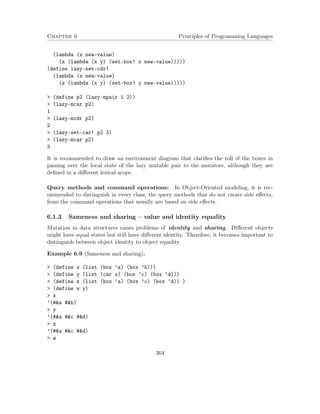
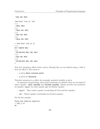
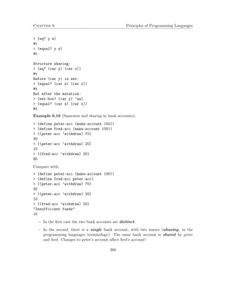
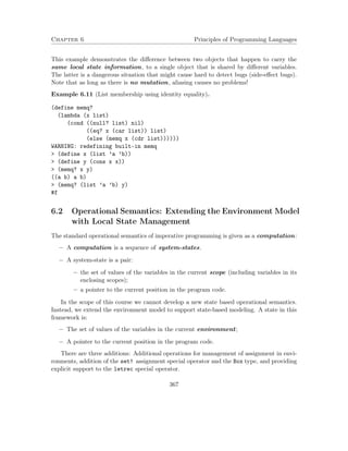
![Chapter 6 Principles of Programming Languages
1. In the environment data structure:
Addition of an operation (command) for setting the value of an already defined vari-able:
set-binding! : [Variable*Scheme-type*Env - Void]
The semantics of set-binding! (x; val; hf1; f2; :::; fni) is defined as follows:
if E(x) is defined
then for the frame fi, such that:
fi(x) is defined while fj(x) is undefined for 1 j i,
set fi(x) = val
else Error
2. Addition of the set! special operator and the Box type:
env eval[(set!xe); env] = set binding!(x; env eval[e; env]; env)
Addition of the primitive procedures of the Box type.
3. Evaluation of a letrec form, as described below.
Evaluation of letrec: In functional programming (substitution or environment model),
recursion is computed by rewriting the code (for example, by adding the function closure
as a parameter, or introducing a fix-point parameter). For that reason, the operational
semantics described in Chapter 2 does not handle recursion in inner scopes. For the global
scope we explicitly added the global-environment mapping, which is defined by application
of define forms.
For recursive global procedures, the define special operator extends the global-environment
mapping with a binding of a variable f and a closure that carries the global-environment
(which is defined on f). Therefore, occurrences of f in the body of this closure are bound by
the declaration of f in the global-environment mapping. But, for locally defined recursive
procedures we had no similar provision.
Consider:
1. (define f (lambda ....))
2. (let ((f (lambda (...) (... (f...)...)))))
3. (f ...)
Mark the declaration on line (1) as f1, and the declaration on line (2) as f2. Then, the
binding of a let form is:
1. (define f1 (lambda ....))
2. (let ((f2 (lambda (...) (... (f1...)...)))))
3. (f2 ...)
while the intended semantics of recursion requires:
368](https://image.slidesharecdn.com/principlesofprogramminglanguages-140901163422-phpapp01/85/Principles-of-programming-languages-373-320.jpg)
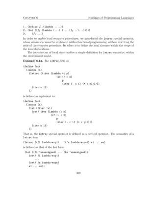
![Chapter 6 Principles of Programming Languages
Static (lexical) observation: The lambda expressions that create the closures for the
local procedures reside within the let scope, and therefore, occurrences of the let variables
in these expressions are bound by the let declarations:
(define f1 (lambda ....))
(let ((f2 ’unassigned))
(set! f2 (lambda (...) (... (f2...)...)))
(f2 ...))
Dynamic (evaluation) observation: The created closures carry the environment that
corresponds to the external let scope, in which the local variable f2 is initialized to a Box
value.
env-eval[(letrec ((f1 lambda-exp1) ...(fn lambda-expn)) e1 ... em), env] =
env-eval[(let ((f1 (box ’unassigned)) ... (fn (box ’unassigned)))
(set! f1 lambda-exp1)
...
(set! fn lambda-expn)
e1 ... em),
env ]
That is, letrec is defined as a derived operator. It is translated into a let form, in
which the internal function names are not initialized. The function definitions are evaluated
within the let body, i.e., with respect to an environment that includes all the letrec declared
variables.
Draw an environment diagram!
6.3 Extending the Environment Model Interpreter and Com-piler
6.3.1 Imperative evaluator
The changes are:
1. Adding support for assignment in the environment data structure: Add
support for changing the value of a variable in an environment, and add the procedures
of the Box type to the external variable the-global-environment.
The modification is in the data structures module env-ds.rkt. Recall that an environ-ment
is implemented as a list of boxed frames (the last being the global environment).
Therefore, it is possible to change frames within this list, without affecting clients of
the environment
370](https://image.slidesharecdn.com/principlesofprogramminglanguages-140901163422-phpapp01/85/Principles-of-programming-languages-375-320.jpg)
![Chapter 6 Principles of Programming Languages
Variable setting in an environment is implemented by the mutating operation set-binding-in-env
which searches for the first frame in which the given variable is defined, and changes
the binding of this variable to the given value.
; Environment mutator: ADT type is [Env*Var - Void]
; Purpose: If the environment is defined on the given variable, set its value
; Type: [Symbol*LIST(Box(Frame)*Var*Scheme-type) - Void]
;Implementation: Uses the get-value-of-variable selector of Substitution, which
; is changed to return a special value ’_not-found’ if variable
; is not defined in the substitution (instead of triggering ’error).
; This is done to allow lookup in an enclosing environment.
(define set-binding-in-env!
(lambda (env var val)
(letrec ((defined-in-env ; ADT type is [Var*Env - Box(Frame) union {empty}]
(lambda (var env)
(if (empty-env? env)
env
(let ((b (get-value-of-variable (first-frame env) var)))
(if (eq? b ’_not-found)
(defined-in-env var (enclosing-env env))
(first-boxed-frame env)))))))
(let ((boxed-frame (defined-in-env var env)))
(if (empty? boxed-frame)
(error ’set! variable not found: ~sn env = ~s var env)
(let ((frame (unbox boxed-frame)))
(set-box! boxed-frame
(change-frame (make-binding var val) frame))))))
))
This operation calls the new change-frame constructor, which creates a new frame,
in which the value of the variable is changed to the given value. change-frame calls a
new substitution mutator change-sub, for creating a new substitution with a modified
value for the given variable. In practice, the value is not changed, but the new binding
is added at the head of the new substitution, so that the lookup selector returns the
new value.
2. Modifying env-eval to support the set! special operator: In the core module
interpreter-core.rkt: Evaluation of assignments calls the new environment muta-tor:
(define eval-assignment
371](https://image.slidesharecdn.com/principlesofprogramminglanguages-140901163422-phpapp01/85/Principles-of-programming-languages-376-320.jpg)
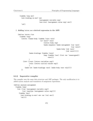
![Chapter 6 Principles of Programming Languages
6.4 Type checking/Inference with assignments:
Typing begin expressions: In an imperative programming paradigm the special operator
begin gains importance. Its typing rule:
Typing rule begin :
For every type environment Tenv,
expressions e1, ..., en, and
type expressions S1, ..., Sn:
If Tenv |- e1:T1, ..., TA |- en:Tn
Then Tenv |- (begin e1 ... en):Tn
Typing set! expressions: An assignment (set! x e) is well typed if e is well typed.
We can further require that the type of e is the type of the variable x, although this
requirement is not enforced by Scheme.
Unlike for definition expressions, assignment expressions must have a derived type, since
they may be nested within other expressions. Therefore, there is a typing rule for assign-ments.
We adopt the more restricting version, that enforces a common type for the variable
and the expression. The type of the assignment expression is always Void.
Typing rule set! :
For every: type assignment TA,
expression e, and
type expression S:
If Tenv |- e:S,
Tenv |- x:S,
Then Tenv |- (set! x e):Void
Example 6.13. Derive a type for:
(lambda (balance)
(lambda (amount)
(if (= balance amount)
(begin (set! balance (- balance amount))
balance)
’Insufficient- funds)))
Typing statements for the leaves balance, amount, - are obtained by instantiating the
Variable, Symbol and Primitive procedure axioms:
1. {balance:T1} |- balance:T1
2. {amount:T2} |- balance:T2
3. {} |- -:[Number*Number - Number]
373](https://image.slidesharecdn.com/principlesofprogramminglanguages-140901163422-phpapp01/85/Principles-of-programming-languages-378-320.jpg)
![Chapter 6 Principles of Programming Languages
4. {} |- ’Insufficient-funds:Symbol
5. {} |- =:[Number*Number - Number]
Applying typing rule Application to typing statements 1,2,3, with type substitution {T1=T2=Number}:
6. {balance:Number, amount:Number} |- (- balance amount):Number
Applying typing rule set! to typing statement 6:
7. {balance:Number, amount:Number} |-
(set! balance (- balance amount)):unit
Applying typing rule begin to typing statements 1,7, with type substitution {T1=Number}:
8. {balance:Number, amount:Number} |-
(begin (set! balance (- balance amount))
balance):Number
Applying typing rule Application to typing statements 1,2,7, with type substitution {T1=T2=Number}:
9. {balance:Number, amount:Number} |- (= balance amount):Number
Applying typing rule If to typing statements 6,7,9:
10. {balance:Number, amount:Number} |-
(if (= balance amount)
(begin (set! balance (- balance amount))
balance)
’Insufficient- funds):Number union Symbol
Applying typing rule Procedure to typing statement 10:
11. {balance:Number} |-
(lambda (amount)
(if (= balance amount)
(begin (set! balance (- balance amount))
balance)
’Insufficient- funds)):[Number - Number union Symbol]
Applying typing rule Procedure to typing statement 11:
12. {} |-
(lambda (balance)
(lambda (amount)
(if (= balance amount)
(begin (set! balance (- balance amount))
balance)
’Insufficient- funds))) :
[Number - [Number - Number union Symbol]]
374](https://image.slidesharecdn.com/principlesofprogramminglanguages-140901163422-phpapp01/85/Principles-of-programming-languages-379-320.jpg)
![Chapter 6 Principles of Programming Languages
Type checking/inference with the Box type: The Box operations are Racket prim-itives.
Therefore, the Primitive procedure typing axiom has to be extended for the new
primitives.
For every type environment Tenv and type expression S:
Tenv |- box:[S - BOX(S)]
Tenv |- unbox:[BOX(S) - S]
Tenv |- set-box!:[BOX(S)*S - Void]
Tenv |- box?:[S - Boolean]
Tenv |- equal?:[BOX(S)*BOX(S) - Boolean]
Tenv |- eq?:[BOX(S)*BOX(S) - Boolean]
6.5 Costs of Introducing Mutation
Languages that are characterized as functional languages (like Scheme and ML) have
operational semantics that is based on successive procedure applications (reductions). The
main syntactic components are expression and function. The main semantic notion is
reduction. Introducing mutation to such languages sharpens the fundamental difference
between expressions that compute values, to side effect language constructs that are
evaluated for the sake of their side effects and not for their returned values.
Languages that are characterized as imperative languages (like Pascal, C, C++, Java)
have operational semantics that is based on successive evaluation of program statements
(or commands). The main syntactic component is the statement, whose evaluation carries
a side effect. The distinction between value returning expressions to side effect commands
is usually blurred. The main semantic element is the state, which is given by the variable
values.
Function call in functional languages is, usually characterized as call-by-value: The
argument expressions are evaluated, and the resulting values are bound to the corresponding
function parameters. Function call in imperative languages is, often, characterized as call-by-
reference: A function receives implicit references to arguments, rather than copy of
their values, and can modify the arguments held by its caller.
6.5.1 Losing Referential Transparency
Languages where equals can be substituted for equals are called referentially trans-parent.
The static analysis support for such language is much simpler and reliable than for
languages that are not referentially transparent.
In referentially transparent languages programs can be compared and simplified by
substituting complex expressions by simpler equal expressions.
375](https://image.slidesharecdn.com/principlesofprogramminglanguages-140901163422-phpapp01/85/Principles-of-programming-languages-380-320.jpg)
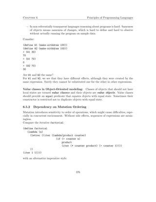
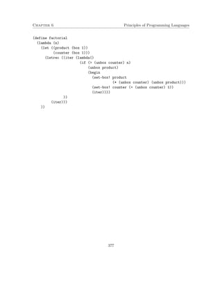
![References Principles of Programming Languages
References
[1] H. Abelson and G.J. Sussman. Structure and Interpretation of Computer Programs,
2nd edition. The MIT Press, 1996.
[2] M. Felleisen, R.B. Findler, M. Flatt, and S. Krishnamurthi. How to Design Programs.
The MIT Press, 2001.
[3] D.P. Friedman and M. Wand. Essentials of Programming Languages, 3nd edition. The
MIT Press, 2008.
[4] E. Gamma, R. Helm, R. Johnson, and J. Vlissides. Design Patterns: Elements of
Reusable Object-Oriented Software. Addison-wesley Reading, MA, 1995.
[5] S. Gilmore. Programming in Standard ML’97: A Tutorial Introduction. Laboratory for
Foundations of Computer Science, The University of Edinburgh, 1997.
[6] R. Harper. Programming in Standard ML. Carnegie Mellon University, 2011.
[7] R. Kowalski. Predicate Logic as a Programming Language, Information Processing 74.
In Proceedings of the IFIP Congress, pages 569–574, 1974.
[8] S. Krishnamurthi. Programming Languages: Application and Interpretation. Version
26, 2007.
[9] OMG. The UML 2.0 Superstructure Specification. Specification Version 2, Object
Management Group, 2007.
[10] L.C. Paulson. ML for the Working Programmer, 2nd edition. Cambridge University
Press, 1996.
[11] L. Sterling and E.Y. Shapiro. The Art of Prolog: Advanced Programming Techniques,
2nd edition. The MIT Press, 1994.
[12] Wikipedia. UML. http://en.wikipedia.org/wiki/Unified_Modeling_Language,
2011.
382](https://image.slidesharecdn.com/principlesofprogramminglanguages-140901163422-phpapp01/85/Principles-of-programming-languages-387-320.jpg)