Downloaded 38 times


![1.5. SUMMARY OF CHAPTER 1 17
to that of the user in question, and see what they liked (a technique known as
collaborative filtering).
1.5 Summary of Chapter 1
3 Data Mining: This term refers to the process of extracting useful models
of data. Sometimes, a model can be a summary of the data, or it can be
the set of most extreme features of the data.
3 Bonferroni’s Principle: If we are willing to view as an interesting feature
of data something of which many can be expected to exist in random data,
then we cannot rely on such features being significant. This observation
limits our ability to mine data for features that are not sufficiently rare
in practice.
3 TF.IDF : The measure called TF.IDF lets us identify words in a collection
of documents that are useful for determining the topic of each document.
A word has high TF.IDF score in a document if it appears in relatively few
documents, but appears in this one, and when it appears in a document
it tends to appear many times.
3 Hash Functions: A hash function maps hash-keys of some data type to
integer bucket numbers. A good hash function distributes the possible
hash-key values approximately evenly among buckets. Any data type can
be the domain of a hash function.
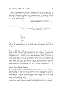
3 Indexes: An index is a data structure that allows us to store and retrieve
data records efficiently, given the value in one or more of the fields of the
record. Hashing is one way to build an index.
3 Storage on Disk : When data must be stored on disk (secondary memory),
it takes very much more time to access a desired data item than if the same
data were stored in main memory. When data is large, it is important
that algorithms strive to keep needed data in main memory.
3 Power Laws: Many phenomena obey a law that can be expressed as
y = cxa for some power a, often around −2. Such phenomena include the
sales of the xth most popular book, or the number of in-links to the xth
most popular page.
1.6 References for Chapter 1
[7] is a clear introduction to the basics of data mining. [2] covers data mining
principally from the point of view of machine learning and statistics.
For construction of hash functions and hash tables, see [4]. Details of the
TF.IDF measure and other matters regarding document processing can be](https://image.slidesharecdn.com/miningofmassivedatasets-120805173332-phpapp01/85/Mining-of-massive-datasets-33-320.jpg)
![18 CHAPTER 1. DATA MINING
found in [5]. See [3] for more on managing indexes, hash tables, and data
on disk.
Power laws pertaining to the Web were explored by [1]. The Matthew effect
was first observed in [6].
1. A. Broder, R. Kumar, F. Maghoul, P. Raghavan, S. Rajagopalan, R.
Stata, A. Tomkins, and J. Weiner, “Graph structure in the web,” Com-
puter Networks 33:1–6, pp. 309–320, 2000.
2. M.M. Gaber, Scientific Data Mining and Knowledge Discovery — Prin-
ciples and Foundations, Springer, New York, 2010.
3. H. Garcia-Molina, J.D. Ullman, and J. Widom, Database Systems: The
Complete Book Second Edition, Prentice-Hall, Upper Saddle River, NJ,
2009.
4. D.E. Knuth, The Art of Computer Programming Vol. 3 (Sorting and
Searching), Second Edition, Addison-Wesley, Upper Saddle River, NJ,
1998.
5. C.P. Manning, P. Raghavan, and H. Sch¨ tze, Introduction to Information
u
Retrieval, Cambridge Univ. Press, 2008.
6. R.K. Merton, “The Matthew effect in science,” Science 159:3810, pp. 56–
63, Jan. 5, 1968.
7. P.-N. Tan, M. Steinbach, and V. Kumar, Introduction to Data Mining,
Addison-Wesley, Upper Saddle River, NJ, 2005.](https://image.slidesharecdn.com/miningofmassivedatasets-120805173332-phpapp01/85/Mining-of-massive-datasets-34-320.jpg)
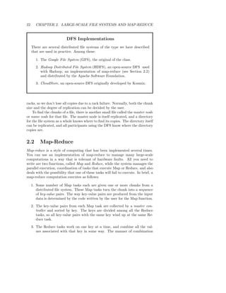
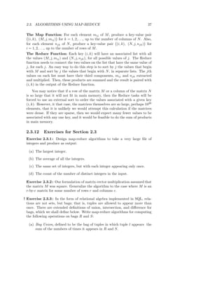
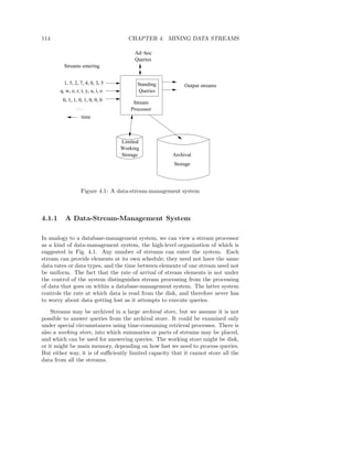
![2.2. MAP-REDUCE 23
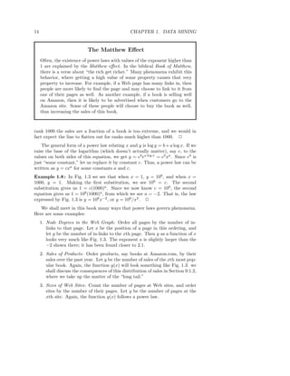
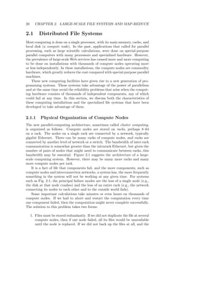
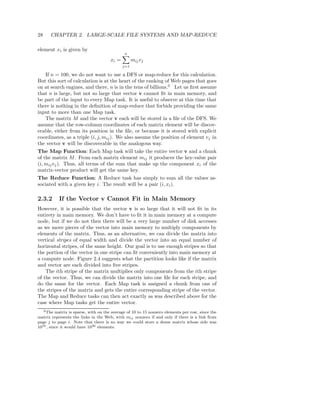
of values is determined by the code written by the user for the Reduce
function.
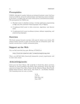
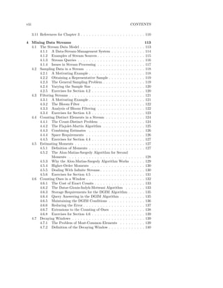
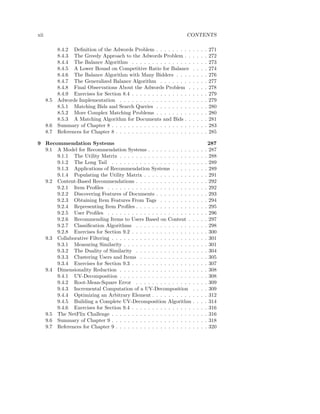
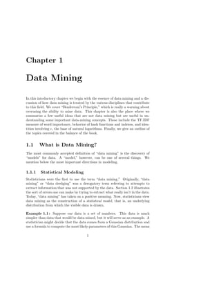
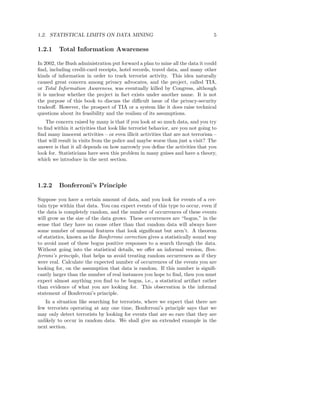
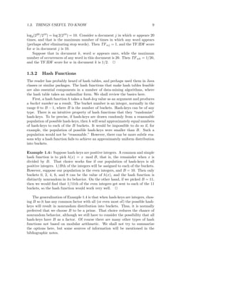
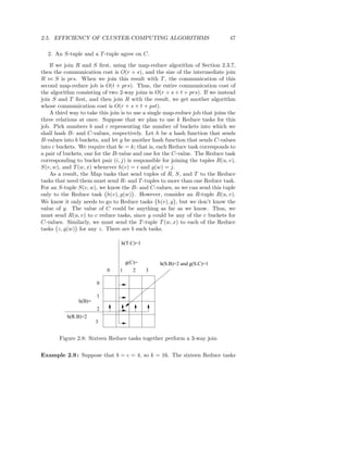
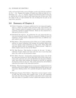
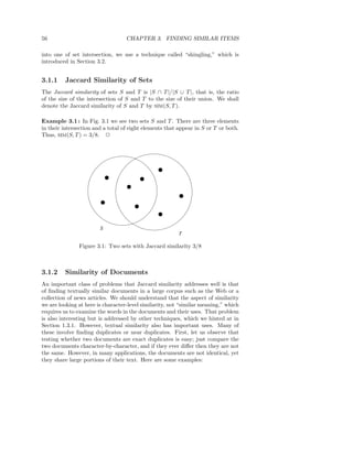
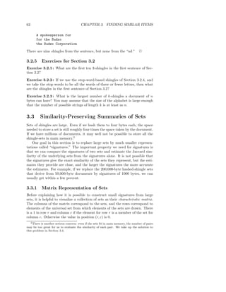
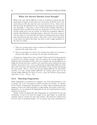
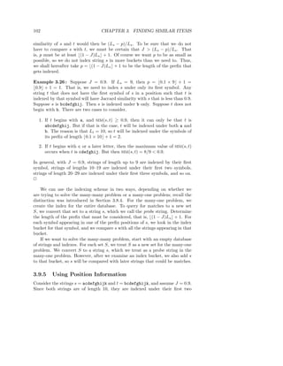
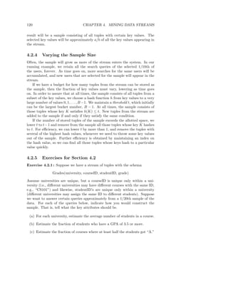
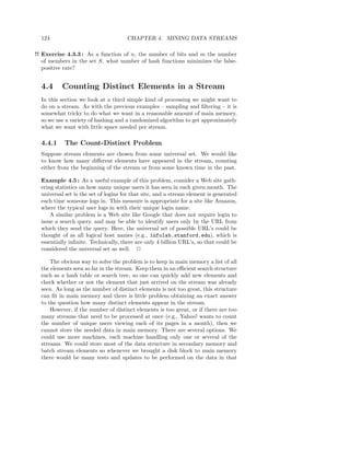
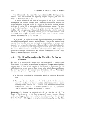
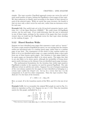
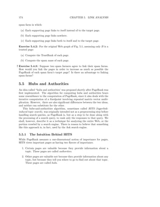
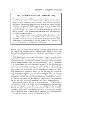
Figure 2.2 suggests this computation.
Keys with all
their values
Key−value
pairs (k, [v, w,...])
Input (k,v)
chunks
Combined
output
Map Group
tasks by keys
Reduce
tasks
Figure 2.2: Schematic of a map-reduce computation
2.2.1 The Map Tasks
We view input files for a Map task as consisting of elements, which can be
any type: a tuple or a document, for example. A chunk is a collection of
elements, and no element is stored across two chunks. Technically, all inputs
to Map tasks and outputs from Reduce tasks are of the key-value-pair form,
but normally the keys of input elements are not relevant and we shall tend to
ignore them. Insisting on this form for inputs and outputs is motivated by the
desire to allow composition of several map-reduce processes.
A Map function is written to convert input elements to key-value pairs. The
types of keys and values are each arbitrary. Further, keys are not “keys” in the
usual sense; they do not have to be unique. Rather a Map task can produce
several key-value pairs with the same key, even from the same element.
Example 2.1 : We shall illustrate a map-reduce computation with what has
become the standard example application: counting the number of occurrences
for each word in a collection of documents. In this example, the input file is a
repository of documents, and each document is an element. The Map function
for this example uses keys that are of type String (the words) and values that](https://image.slidesharecdn.com/miningofmassivedatasets-120805173332-phpapp01/85/Mining-of-massive-datasets-39-320.jpg)
![24 CHAPTER 2. LARGE-SCALE FILE SYSTEMS AND MAP-REDUCE
are integers. The Map task reads a document and breaks it into its sequence
of words w1 , w2 , . . . , wn . It then emits a sequence of key-value pairs where the
value is always 1. That is, the output of the Map task for this document is the
sequence of key-value pairs:
(w1 , 1), (w2 , 1), . . . , (wn , 1)
Note that a single Map task will typically process many documents – all
the documents in one or more chunks. Thus, its output will be more than the
sequence for the one document suggested above. Note also that if a word w
appears m times among all the documents assigned to that process, then there
will be m key-value pairs (w, 1) among its output. An option, which we discuss
in Section 2.2.4, is to combine these m pairs into a single pair (w, m), but we
can only do that because, as we shall see, the Reduce tasks apply an associative
and commutative operation, addition, to the values. 2
2.2.2 Grouping and Aggregation
Grouping and aggregation is done the same way, regardless of what Map and
Reduce tasks do. The master controller process knows how many Reduce tasks
there will be, say r such tasks. The user typically tells the map-reduce system
what r should be. Then the master controller normally picks a hash function
that applies to keys and produces a bucket number from 0 to r − 1. Each key
that is output by a Map task is hashed and its key-value pair is put in one of
r local files. Each file is destined for one of the Reduce tasks.1
After all the Map tasks have completed successfully, the master controller
merges the file from each Map task that are destined for a particular Reduce
task and feeds the merged file to that process as a sequence of key-list-of-value
pairs. That is, for each key k, the input to the Reduce task that handles key
k is a pair of the form (k, [v1 , v2 , . . . , vn ]), where (k, v1 ), (k, v2 ), . . . , (k, vn ) are
all the key-value pairs with key k coming from all the Map tasks.
2.2.3 The Reduce Tasks
The Reduce function is written to take pairs consisting of a key and its list
of associated values and combine those values in some way. The output of a
Reduce task is a sequence of key-value pairs consisting of each input key k that
the Reduce task received, paired with the combined value constructed from the
list of values that the Reduce task received along with key k. The outputs from
all the Reduce tasks are merged into a single file.
Example 2.2 : Let us continue with the word-count example of Example 2.1.
The Reduce function simply adds up all the values. Thus, the output of the
1 Optionally, users can specify their own hash function or other method for assigning keys
to Reduce tasks. However, whatever algorithm is used, each key is assigned to one and only
one Reduce task.](https://image.slidesharecdn.com/miningofmassivedatasets-120805173332-phpapp01/85/Mining-of-massive-datasets-40-320.jpg)
![32 CHAPTER 2. LARGE-SCALE FILE SYSTEMS AND MAP-REDUCE
Friends(User, Friend)
This relation has tuples that are pairs (a, b) such that b is a friend of a. The site
might want to develop statistics about the number of friends members have.
Their first step would be to compute a count of the number of friends of each
user. This operation can be done by grouping and aggregation, specifically
γUser,COUNT(Friend) (Friends)
This operation groups all the tuples by the value in their first component, so
there is one group for each user. Then, for each group the count of the number
of friends of that user is made.5 The result will be one tuple for each group,
and a typical tuple would look like (Sally, 300), if user “Sally” has 300 friends.
2
2.3.4 Computing Selections by Map-Reduce
Selections really do not need the full power of map-reduce. They can be done
most conveniently in the map portion alone, although they could also be done
in the reduce portion alone. Here is a map-reduce implementation of selection
σC (R).
The Map Function: For each tuple t in R, test if it satisfies C. If so, produce
the key-value pair (t, t). That is, both the key and value are t.
The Reduce Function: The Reduce function is the identity. It simply passes
each key-value pair to the output.
Note that the output is not exactly a relation, because it has key-value pairs.
However, a relation can be obtained by using only the value components (or
only the key components) of the output.
2.3.5 Computing Projections by Map-Reduce
Projection is performed similarly to selection, because projection may cause
the same tuple to appear several times, the Reduce function must eliminate
duplicates. We may compute πS (R) as follows.
The Map Function: For each tuple t in R, construct a tuple t′ by eliminating
from t those components whose attributes are not in S. Output the key-value
pair (t′ , t′ ).
The Reduce Function: For each key t′ produced by any of the Map tasks,
there will be one or more key-value pairs (t′ , t′ ). The Reduce function turns
(t′ , [t′ , t′ , . . . , t′ ]) into (t′ , t′ ), so it produces exactly one pair (t′ , t′ ) for this key
t′ .
5 The COUNT operation applied to an attribute does not consider the values of that
attribute, so it is really counting the number of tuples in the group. In SQL, there is a
count-distinct operator that counts the number of different values, but we do not discuss this
operator here.](https://image.slidesharecdn.com/miningofmassivedatasets-120805173332-phpapp01/85/Mining-of-massive-datasets-48-320.jpg)
![2.3. ALGORITHMS USING MAP-REDUCE 33
Observe that the Reduce operation is duplicate elimination. This operation
is associative and commutative, so a combiner associated with each Map task
can eliminate whatever duplicates are produced locally. However, the Reduce
tasks are still needed to eliminate two identical tuples coming from different
Map tasks.
2.3.6 Union, Intersection, and Difference by Map-Reduce
First, consider the union of two relations. Suppose relations R and S have the
same schema. Map tasks will be assigned chunks from either R or S; it doesn’t
matter which. The Map tasks don’t really do anything except pass their input
tuples as key-value pairs to the Reduce tasks. The latter need only eliminate
duplicates as for projection.
The Map Function: Turn each input tuple t into a key-value pair (t, t).
The Reduce Function: Associated with each key t there will be either one or
two values. Produce output (t, t) in either case.
To compute the intersection, we can use the same Map function. However,
the Reduce function must produce a tuple only if both relations have the tuple.
If the key t has two values [t, t] associated with it, then the Reduce task for
t should produce (t, t). However, if the value associated with key t is just [t],
then one of R and S is missing t, so we don’t want to produce a tuple for the
intersection. We need to produce a value that indicates “no tuple,” such as the
SQL value NULL. When the result relation is constructed from the output, such
a tuple will be ignored.
The Map Function: Turn each tuple t into a key-value pair (t, t).
The Reduce Function: If key t has value list [t, t], then produce (t, t). Oth-
erwise, produce (t, NULL).
The Difference R − S requires a bit more thought. The only way a tuple
t can appear in the output is if it is in R but not in S. The Map function
can pass tuples from R and S through, but must inform the Reduce function
whether the tuple came from R or S. We shall thus use the relation as the
value associated with the key t. Here is a specification for the two functions.
The Map Function: For a tuple t in R, produce key-value pair (t, R), and for
a tuple t in S, produce key-value pair (t, S). Note that the intent is that the
value is the name of R or S, not the entire relation.
The Reduce Function: For each key t, do the following.
1. If the associated value list is [R], then produce (t, t).
2. If the associated value list is anything else, which could only be [R, S],
[S, R], or [S], produce (t, NULL).](https://image.slidesharecdn.com/miningofmassivedatasets-120805173332-phpapp01/85/Mining-of-massive-datasets-49-320.jpg)
![34 CHAPTER 2. LARGE-SCALE FILE SYSTEMS AND MAP-REDUCE
2.3.7 Computing Natural Join by Map-Reduce
The idea behind implementing natural join via map-reduce can be seen if we
look at the specific case of joining R(A, B) with S(B, C). We must find tuples
that agree on their B components, that is the second component from tuples
of R and the first component of tuples of S. We shall use the B-value of tuples
from either relation as the key. The value will be the other component and the
name of the relation, so the Reduce function can know where each tuple came
from.
The Map Function: For each tuple (a, b) of R, produce the key-value pair
b, (R, a) . For each tuple (b, c) of S, produce the key-value pair b, (S, c) .
The Reduce Function: Each key value b will be associated with a list of pairs
that are either of the form (R, a) or (S, c). Construct all pairs consisting of one
with first component R and the other with first component S, say (R, a) and
(S, c). The output for key b is (b, [(a1 , b, c1 ), (a2 , b, c2 ), . . .]), that is, b associated
with the list of tuples that can be formed from an R-tuple and an S-tuple with
a common b value.
There are a few observations we should make about this join algorithm.
First, the relation that is the result of the join is recovered by taking all the
tuples that appear on the lists for any key. Second, map-reduce implementations
such as Hadoop pass values to the Reduce tasks sorted by key. If so, then
identifying all the tuples from both relations that have key b is easy. If another
implementation were not to provide key-value pairs sorted by key, then the
Reduce function could still manage its task efficiently by hashing key-value
pairs locally by key. If enough buckets were used, most buckets would have
only one key. Finally, if there are n tuples of R with B-value b and m tuples
from S with B-value b, then there are mn tuples with middle component b in
the result. In the extreme case, all tuples from R and S have the same b-value,
and we are really taking a Cartesian product. However, it is quite common for
the number of tuples with shared B-values to be small, and in that case, the
time complexity of the Reduce function is closer to linear in the relation sizes
than to quadratic.
2.3.8 Generalizing the Join Algorithm
The same algorithm works if the relations have more than two attributes. You
can think of A as representing all those attributes in the schema of R but not
S. B represents the attributes in both schemas, and C represents attributes
only in the schema of S. The key for a tuple of R or S is the list of values in all
the attributes that are in the schemas of both R and S. The value for a tuple
of R is the name R and the values of all the attributes of R but not S, and the
value for a tuple of S is the name S and the values of the attributes of S but
not R.
The Reduce function looks at all the key-value pairs with a given key and
combines those values from R with those values of S in all possible ways. From](https://image.slidesharecdn.com/miningofmassivedatasets-120805173332-phpapp01/85/Mining-of-massive-datasets-50-320.jpg)
![2.3. ALGORITHMS USING MAP-REDUCE 35
each pairing, the tuple produced has the values from R, the key values, and the
values from S.
2.3.9 Grouping and Aggregation by Map-Reduce
As with the join, we shall discuss the minimal example of grouping and aggrega-
tion, where there is one grouping attribute and one aggregation. Let R(A, B, C)
be a relation to which we apply the operator γA,θ(B) (R). Map will perform the
grouping, while Reduce does the aggregation.
The Map Function: For each tuple (a, b, c) produce the key-value pair (a, b).
The Reduce Function: Each key a represents a group. Apply the aggregation
operator θ to the list [b1 , b2 , . . . , bn ] of B-values associated with key a. The
output is the pair (a, x), where x is the result of applying θ to the list. For
example, if θ is SUM, then x = b1 + b2 + · · · + bn , and if θ is MAX, then x is
the largest of b1 , b2 , . . . , bn .
If there are several grouping attributes, then the key is the list of the values
of a tuple for all these attributes. If there is more than one aggregation, then
the Reduce function applies each of them to the list of values associated with
a given key and produces a tuple consisting of the key, including components
for all grouping attributes if there is more than one, followed by the results of
each of the aggregations.
2.3.10 Matrix Multiplication
If M is a matrix with element mij in row i and column j, and N is a matrix
with element njk in row j and column k, then the product P = M N is the
matrix P with element pik in row i and column k, where
pik = mij njk
j
It is required that the number of columns of M equals the number of rows of
N , so the sum over j makes sense.
We can think of a matrix as a relation with three attributes: the row number,
the column number, and the value in that row and column. Thus, we could
view matrix M as a relation M (I, J, V ), with tuples (i, j, mij ) and we could view
matrix N as a relation N (J, K, W ), with tuples (j, k, njk ). As large matrices are
often sparse (mostly 0’s), and since we can omit the tuples for matrix elements
that are 0, this relational representation is often a very good one for a large
matrix. However, it is possible that i, j, and k are implicit in the position of a
matrix element in the file that represents it, rather than written explicitly with
the element itself. In that case, the Map function will have to be designed to
construct the I, J, and K components of tuples from the position of the data.
The product M N is almost a natural join followed by grouping and ag-
gregation. That is, the natural join of M (I, J, V ) and N (J, K, W ), having](https://image.slidesharecdn.com/miningofmassivedatasets-120805173332-phpapp01/85/Mining-of-massive-datasets-51-320.jpg)
![36 CHAPTER 2. LARGE-SCALE FILE SYSTEMS AND MAP-REDUCE
only attribute J in common, would produce tuples (i, j, k, v, w) from each tuple
(i, j, v) in M and tuple (j, k, w) in N . This five-component tuple represents the
pair of matrix elements (mij , njk ). What we want instead is the product of
these elements, that is, the four-component tuple (i, j, k, v × w), because that
represents the product mij njk . Once we have this relation as the result of one
map-reduce operation, we can perform grouping and aggregation, with I and
K as the grouping attributes and the sum of V × W as the aggregation. That
is, we can implement matrix multiplication as the cascade of two map-reduce
operations, as follows. First:
The Map Function: Send each matrix element mij to the key value pair
j, (M, i, mij )
Send each matrix element njk to the key value pair j, (N, k, njk ) .
The Reduce Function: For each key j, examine its list of associated values.
For each value that comes from M , say (M, i, mij ) , and each value that comes
from N , say (N, k, njk ) , produce the tuple (i, k, mij njk ). Note that the output
of the Reduce function is a key j paired with the list of all the tuples of this
form that we get from j.
Now, we perform a grouping and aggregation by another map-reduce operation.
The Map Function: The elements to which this Map function is applied are
the pairs that are output from the previous Reduce function. These pairs are
of the form
(j, [(i1 , k1 , v1 ), (i2 , k2 , v2 ), . . . , (ip , kp , vp )]
where each vq is the product of elements miq j and njkq . From this element we
produce p key-value pairs:
(i1 , k1 ), v1 , (i2 , k2 ), v2 , . . . , (ip , kp ), vp
The Reduce Function: For each key (i, k), produce the sum of the list of
values associated with this key. The result is a pair (i, k), v , where v is the
value of the element in row i and column k of the matrix P = M N .
2.3.11 Matrix Multiplication with One Map-Reduce Step
There often is more than one way to use map-reduce to solve a problem. You
may wish to use only a single map-reduce pass to perform matrix multiplication
P = M N . It is possible to do so if we put more work into the two functions.
Start by using the Map function to create the sets of matrix elements that are
needed to compute each element of the answer P . Notice that an element of
M or N contributes to many elements of the result, so one input element will
be turned into many key-value pairs. The keys will be pairs (i, k), where i is a
row of M and k is a column of N . Here is a synopsis of the Map and Reduce
functions.](https://image.slidesharecdn.com/miningofmassivedatasets-120805173332-phpapp01/85/Mining-of-massive-datasets-52-320.jpg)
![52 CHAPTER 2. LARGE-SCALE FILE SYSTEMS AND MAP-REDUCE
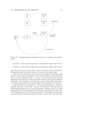
possible repetition of the effects of that task. It is necessary to restart the
entire job only if the node at which the Master executes fails.
3 Applications of Map-Reduce: While not all parallel algorithms are suitable
for implementation in the map-reduce framework, there are simple imple-
mentations of matrix-vector and matrix-matrix multiplication. Also, the
principal operators of relational algebra are easily implemented in map-
reduce.
3 Workflow Systems: Map-reduce has been generalized to systems that sup-
port any acyclic collection of functions, each of which can be instantiated
by any number of tasks, each responsible for executing that function on a
portion of the data. Clustera and Hyracks are examples of such systems.
3 Recursive Workflows: When implementing a recursive collection of func-
tions, it is not always possible to preserve the ability to restart any failed
task, because recursive tasks may have produced output that was con-
sumed by another task before the failure. A number of schemes for check-
pointing parts of the computation to allow restart of single tasks, or restart
all tasks from a recent point, have been proposed.
3 The Communication-Cost Model : Many applications of map-reduce or
similar systems do very simple things for each task. Then, the dominant
cost is usually the cost of transporting data from where it is created to
where it is used. In these cases, efficiency of an algorithm can be estimated
by calculating the sum of the sizes of the inputs to all the tasks.
3 Multiway Joins: It is sometimes more efficient to replicate tuples of the
relations involved in a join and have the join of three or more relations
computed as a single map-reduce job. The technique of Lagrangean mul-
tipliers can be used to optimize the degree of replication for each of the
participating relations.
3 Star Joins: Analytic queries often involve a very large fact table joined
with smaller dimension tables. These joins can always be done efficiently
by the multiway-join technique. An alternative is to distribute the fact
table and replicate the dimension tables permanently, using the same
strategy as would be used if we were taking the multiway join of the fact
table and every dimension table.
2.7 References for Chapter 2
GFS, the Google File System, was described in [10]. The paper on Google’s
map-reduce is [8]. Information about Hadoop and HDFS can be found at [11].
More detail on relations and relational algebra can be found in [16].
Clustera is covered in [9]. Hyracks (previously called Hyrax) is from [4].
The Dryad system [13] has similar capabilities, but requires user creation of](https://image.slidesharecdn.com/miningofmassivedatasets-120805173332-phpapp01/85/Mining-of-massive-datasets-68-320.jpg)
![2.7. REFERENCES FOR CHAPTER 2 53
parallel tasks. That responsibility was automated through the introduction of
DryadLINQ [17]. For a discussion of cluster implementation of recursion, see
[1]. Pregel is from [14].
A different approach to recursion was taken in Haloop [5]. There, recursion
is seen as an iteration, with the output of one round being input to the next
round. Efficiency is obtained by managing the location of the intermediate data
and the tasks that implement each round.
The communication-cost model for algorithms comes from [2]. [3] discusses
optimal implementations of multiway joins using a map-reduce system.
There are a number of other systems built on a distributed file system and/or
map-reduce, which have not been covered here, but may be worth knowing
about. [6] describes BigTable, a Google implementation of an object store of
very large size. A somewhat different direction was taken at Yahoo! with Pnuts
[7]. The latter supports a limited form of transaction processing, for example.
PIG [15] is an implementation of relational algebra on top of Hadoop. Sim-
ilarly, Hive [12] implements a restricted form of SQL on top of Hadoop.
1. F.N. Afrati, V. Borkar, M. Carey, A. Polyzotis, and J.D. Ullman, “Clus-
ter computing, recursion, and Datalog,” to appear in Proc. Datalog 2.0
Workshop, Elsevier, 2011.
2. F.N. Afrati and J.D. Ullman, “A new computation model for cluster com-
puting,” http://ilpubs.stanford.edu:8090/953, Stanford Dept. of CS
Technical Report, 2009.
3. F.N. Afrati and J.D. Ullman, “Optimizing joins in a map-reduce environ-
ment,” Proc. Thirteenth Intl. Conf. on Extending Database Technology,
2010.
4. V. Borkar and M. Carey, “Hyrax: demonstrating a new foundation for
data-parallel computation,”
http://asterix.ics.uci.edu/pub/hyraxdemo.pdf
Univ. of California, Irvine, 2010.
5. Y. Bu, B. Howe, M. Balazinska, and M. Ernst, “HaLoop: efficient iter-
ative data processing on large clusters,” Proc. Intl. Conf. on Very Large
Databases, 2010.
6. F. Chang, J. Dean, S. Ghemawat, W.C. Hsieh, D.A. Wallach, M. Burrows,
T. Chandra, A. Fikes, and R.E. Gruber, “Bigtable: a distributed storage
system for structured data,” ACM Transactions on Computer Systems
26:2, pp. 1–26, 2008.
7. B.F. Cooper, R. Ramakrishnan, U. Srivastava, A. Silberstein, P. Bohan-
non, H.-A. Jacobsen, N. Puz, D. Weaver, and R. Yerneni, “Pnuts: Ya-
hoo!’s hosted data serving platform,” PVLDB 1:2, pp. 1277–1288, 2008.](https://image.slidesharecdn.com/miningofmassivedatasets-120805173332-phpapp01/85/Mining-of-massive-datasets-69-320.jpg)

![3.3. SIMILARITY-PRESERVING SUMMARIES OF SETS 65
3.3.4 Minhash Signatures
Again think of a collection of sets represented by their characteristic matrix M .
To represent sets, we pick at random some number n of permutations of the
rows of M . Perhaps 100 permutations or several hundred permutations will do.
Call the minhash functions determined by these permutations h1 , h2 , . . . , hn .
From the column representing set S, construct the minhash signature for S, the
vector [h1 (S), h2 (S), . . . , hn (S)]. We normally represent this list of hash-values
as a column. Thus, we can form from matrix M a signature matrix, in which
the ith column of M is replaced by the minhash signature for (the set of) the
ith column.
Note that the signature matrix has the same number of columns as M but
only n rows. Even if M is not represented explicitly, but in some compressed
form suitable for a sparse matrix (e.g., by the locations of its 1’s), it is normal
for the signature matrix to be much smaller than M .
3.3.5 Computing Minhash Signatures
It is not feasible to permute a large characteristic matrix explicitly. Even picking
a random permutation of millions or billions of rows is time-consuming, and
the necessary sorting of the rows would take even more time. Thus, permuted
matrices like that suggested by Fig. 3.3, while conceptually appealing, are not
implementable.
Fortunately, it is possible to simulate the effect of a random permutation by
a random hash function that maps row numbers to as many buckets as there
are rows. A hash function that maps integers 0, 1, . . . , k − 1 to bucket numbers
0 through k − 1 typically will map some pairs of integers to the same bucket and
leave other buckets unfilled. However, the difference is unimportant as long as
k is large and there are not too many collisions. We can maintain the fiction
that our hash function h “permutes” row r to position h(r) in the permuted
order.
Thus, instead of picking n random permutations of rows, we pick n randomly
chosen hash functions h1 , h2 , . . . , hn on the rows. We construct the signature
matrix by considering each row in their given order. Let SIG(i, c) be the element
of the signature matrix for the ith hash function and column c. Initially, set
SIG(i, c) to ∞ for all i and c. We handle row r by doing the following:
1. Compute h1 (r), h2 (r), . . . , hn (r).
2. For each column c do the following:
(a) If c has 0 in row r, do nothing.
(b) However, if c has 1 in row r, then for each i = 1, 2, . . . , n set SIG(i, c)
to the smaller of the current value of SIG(i, c) and hi (r).](https://image.slidesharecdn.com/miningofmassivedatasets-120805173332-phpapp01/85/Mining-of-massive-datasets-81-320.jpg)
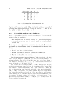
![3.3. SIMILARITY-PRESERVING SUMMARIES OF SETS 67
signature for S4 , but the values in this column of the signature matrix, [1, 1], are
each less than the corresponding hash values [3, 2]. However, since the column
for S2 still has ∞’s, we replace it by [3, 2], resulting in:
S1 S2 S3 S4
h1 1 3 2 1
h2 1 2 4 1
Next comes the row numbered 3 in Fig. 3.4. Here, all columns but S2 have
1, and the hash values are h1 (3) = 4 and h2 (3) = 0. The value 4 for h1 exceeds
what is already in the signature matrix for all the columns, so we shall not
change any values in the first row of the signature matrix. However, the value
0 for h2 is less than what is already present, so we lower SIG(2, 1), SIG(2, 3) and
SIG(2, 4) to 0. Note that we cannot lower SIG(2, 2) because the column for S2 in
Fig. 3.4 has 0 in the row we are currently considering. The resulting signature
matrix:
S1 S2 S3 S4
h1 1 3 2 1
h2 0 2 0 0
Finally, consider the row of Fig. 3.4 numbered 4. h1 (4) = 0 and h2 (4) = 3.
Since row 4 has 1 only in the column for S3 , we only compare the current
signature column for that set, [2, 0] with the hash values [0, 3]. Since 0 < 2, we
change SIG(1, 3) to 0, but since 3 > 0 we do not change SIG(2, 3). The final
signature matrix is:
S1 S2 S3 S4
h1 1 3 0 1
h2 0 2 0 0
We can estimate the Jaccard similarities of the underlying sets from this
signature matrix. Notice that columns 1 and 4 are identical, so we guess that
SIM(S1 , S4 ) = 1.0. If we look at Fig. 3.4, we see that the true Jaccard similarity
of S1 and S4 is 2/3. Remember that the fraction of rows that agree in the
signature matrix is only an estimate of the true Jaccard similarity, and this
example is much too small for the law of large numbers to assure that the
estimates are close. For additional examples, the signature columns for S1 and
S3 agree in half the rows (true similarity 1/4), while the signatures of S1 and
S2 estimate 0 as their Jaccard similarity (the correct value). 2
3.3.6 Exercises for Section 3.3
Exercise 3.3.1 : Verify the theorem from Section 3.3.3, which relates the Jac-
card similarity to the probability of minhashing to equal values, for the partic-
ular case of Fig. 3.2.](https://image.slidesharecdn.com/miningofmassivedatasets-120805173332-phpapp01/85/Mining-of-massive-datasets-83-320.jpg)
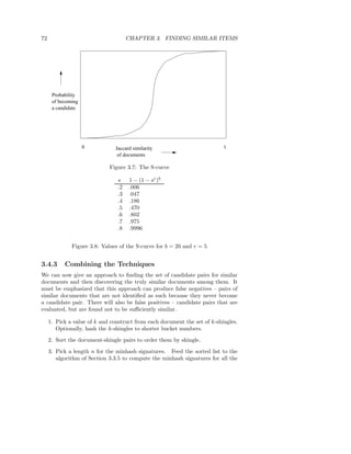
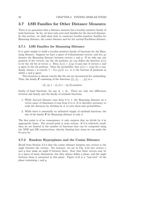
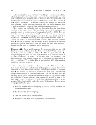
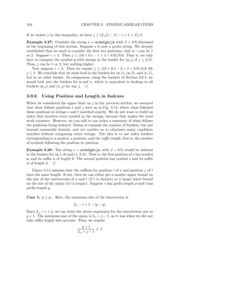
![70 CHAPTER 3. FINDING SIMILAR ITEMS
items are. We then consider any pair that hashed to the same bucket for any
of the hashings to be a candidate pair. We check only the candidate pairs for
similarity. The hope is that most of the dissimilar pairs will never hash to the
same bucket, and therefore will never be checked. Those dissimilar pairs that
do hash to the same bucket are false positives; we hope these will be only a
small fraction of all pairs.. We also hope that most of the truly similar pairs
will hash to the same bucket under at least one of the hash functions. Those
that do not are false negatives; we hope these will be only a small fraction of
the truly similar pairs.
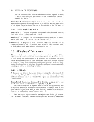
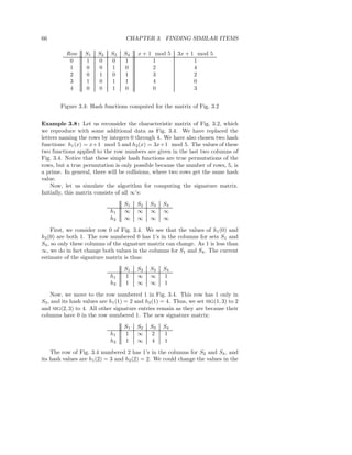
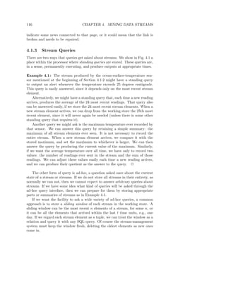
If we have minhash signatures for the items, an effective way to choose the
hashings is to divide the signature matrix into b bands consisting of r rows
each. For each band, there is a hash function that takes vectors of r integers
(the portion of one column within that band) and hashes them to some large
number of buckets. We can use the same hash function for all the bands, but
we use a separate bucket array for each band, so columns with the same vector
in different bands will not hash to the same bucket.
10002
band 1 ... 32122 ...
01311
band 2
band 3
band 4
Figure 3.6: Dividing a signature matrix into four bands of three rows per band
Example 3.10 : Figure 3.6 shows part of a signature matrix of 12 rows divided
into four bands of three rows each. The second and fourth of the explicitly
shown columns each have the column vector [0, 2, 1] in the first band, so they
will definitely hash to the same bucket in the hashing for the first band. Thus,
regardless of what those columns look like in the other three bands, this pair
of columns will be a candidate pair. It is possible that other columns, such as
the first two shown explicitly, will also hash to the same bucket according to
the hashing of the first band. However, since their column vectors are different,
[1, 3, 0] and [0, 2, 1], and there are many buckets for each hashing, we expect the
chances of an accidental collision to be very small. We shall normally assume
that two vectors hash to the same bucket if and only if they are identical.
Two columns that do not agree in band 1 have three other chances to become
a candidate pair; they might be identical in any one of these other bands.](https://image.slidesharecdn.com/miningofmassivedatasets-120805173332-phpapp01/85/Mining-of-massive-datasets-86-320.jpg)

![74 CHAPTER 3. FINDING SIMILAR ITEMS
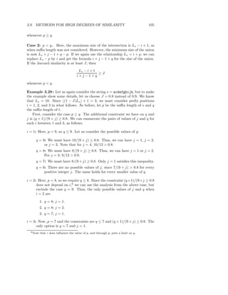
3.5 Distance Measures
We now take a short detour to study the general notion of distance measures.
The Jaccard similarity is a measure of how close sets are, although it is not
really a distance measure. That is, the closer sets are, the higher the Jaccard
similarity. Rather, 1 minus the Jaccard similarity is a distance measure, as we
shall see; it is called the Jaccard distance.
However, Jaccard distance is not the only measure of closeness that makes
sense. We shall examine in this section some other distance measures that have
applications. Then, in Section 3.6 we see how some of these distance measures
also have an LSH technique that allows us to focus on nearby points without
comparing all points. Other applications of distance measures will appear when
we study clustering in Chapter 7.
3.5.1 Definition of a Distance Measure
Suppose we have a set of points, called a space. A distance measure on this
space is a function d(x, y) that takes two points in the space as arguments and
produces a real number, and satisfies the following axioms:
1. d(x, y) ≥ 0 (no negative distances).
2. d(x, y) = 0 if and only if x = y (distances are positive, except for the
distance from a point to itself).
3. d(x, y) = d(y, x) (distance is symmetric).
4. d(x, y) ≤ d(x, z) + d(z, y) (the triangle inequality).
The triangle inequality is the most complex condition. It says, intuitively, that
to travel from x to y, we cannot obtain any benefit if we are forced to travel via
some particular third point z. The triangle-inequality axiom is what makes all
distance measures behave as if distance describes the length of a shortest path
from one point to another.
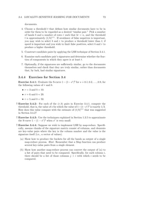
3.5.2 Euclidean Distances
The most familiar distance measure is the one we normally think of as “dis-
tance.” An n-dimensional Euclidean space is one where points are vectors of n
real numbers. The conventional distance measure in this space, which we shall
refer to as the L2 -norm, is defined:
n
d([x1 , x2 , . . . , xn ], [y1 , y2 , . . . , yn ]) = (xi − yi )2
i=1
That is, we square the distance in each dimension, sum the squares, and take
the positive square root.](https://image.slidesharecdn.com/miningofmassivedatasets-120805173332-phpapp01/85/Mining-of-massive-datasets-90-320.jpg)
![3.5. DISTANCE MEASURES 75
It is easy to verify the first three requirements for a distance measure are
satisfied. The Euclidean distance between two points cannot be negative, be-
cause the positive square root is intended. Since all squares of real numbers are
nonnegative, any i such that xi = yi forces the distance to be strictly positive.
On the other hand, if xi = yi for all i, then the distance is clearly 0. Symmetry
follows because (xi − yi )2 = (yi − xi )2 . The triangle inequality requires a good
deal of algebra to verify. However, it is well understood to be a property of
Euclidean space: the sum of the lengths of any two sides of a triangle is no less
than the length of the third side.
There are other distance measures that have been used for Euclidean spaces.
For any constant r, we can define the Lr -norm to be the distance measure d
defined by:
n
d([x1 , x2 , . . . , xn ], [y1 , y2 , . . . , yn ]) = ( |xi − yi |r )1/r
i=1
The case r = 2 is the usual L2 -norm just mentioned. Another common distance
measure is the L1 -norm, or Manhattan distance. There, the distance between
two points is the sum of the magnitudes of the differences in each dimension.
It is called “Manhattan distance” because it is the distance one would have to
travel between points if one were constrained to travel along grid lines, as on
the streets of a city such as Manhattan.
Another interesting distance measure is the L∞ -norm, which is the limit
as r approaches infinity of the Lr -norm. As r gets larger, only the dimension
with the largest difference matters, so formally, the L∞ -norm is defined as the
maximum of |xi − yi | over all dimensions i.
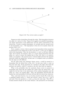
Example 3.12 : Consider the two-dimensional Euclidean space (the custom-
ary plane) and the points √ 7) and (6, 4). The L2 -norm gives a distance
(2,
of (2 − 6)2 + (7 − 4)2 = 42 + 32 = 5. The L1 -norm gives a distance of
|2 − 6| + |7 − 4| = 4 + 3 = 7. The L∞ -norm gives a distance of
max(|2 − 6|, |7 − 4|) = max(4, 3) = 4
2
3.5.3 Jaccard Distance
As mentioned at the beginning of the section, we define the Jaccard distance
of sets by d(x, y) = 1 − SIM(x, y). That is, the Jaccard distance is 1 minus the
ratio of the sizes of the intersection and union of sets x and y. We must verify
that this function is a distance measure.
1. d(x, y) is nonnegative because the size of the intersection cannot exceed
the size of the union.](https://image.slidesharecdn.com/miningofmassivedatasets-120805173332-phpapp01/85/Mining-of-massive-datasets-91-320.jpg)
![76 CHAPTER 3. FINDING SIMILAR ITEMS
2. d(x, y) = 0 if x = y, because x ∪ x = x ∩ x = x. However, if x = y, then
the size of x ∩ y is strictly less than the size of x ∪ y, so d(x, y) is strictly
positive.
3. d(x, y) = d(y, x) because both union and intersection are symmetric; i.e.,
x ∪ y = y ∪ x and x ∩ y = y ∩ x.
4. For the triangle inequality, recall from Section 3.3.3 that SIM(x, y) is the
probability a random minhash function maps x and y to the same value.
Thus, the Jaccard distance d(x, y) is the probability that a random min-
hash function does not send x and y to the same value. We can therefore
translate the condition d(x, y) ≤ d(x, z) + d(z, y) to the statement that if
h is a random minhash function, then the probability that h(x) = h(y)
is no greater than the sum of the probability that h(x) = h(z) and the
probability that h(z) = h(y). However, this statement is true because
whenever h(x) = h(y), at least one of h(x) and h(y) must be different
from h(z). They could not both be h(z), because then h(x) and h(y)
would be the same.
.
3.5.4 Cosine Distance
The cosine distance makes sense in spaces that have dimensions, including Eu-
clidean spaces and discrete versions of Euclidean spaces, such as spaces where
points are vectors with integer components or boolean (0 or 1) components. In
such a space, points may be thought of as directions. We do not distinguish be-
tween a vector and a multiple of that vector. Then the cosine distance between
two points is the angle that the vectors to those points make. This angle will
be in the range 0 to 180 degrees, regardless of how many dimensions the space
has.
We can calculate the cosine distance by first computing the cosine of the
angle, and then applying the arc-cosine function to translate to an angle in the
0-180 degree range. Given two vectors x and y, the cosine of the angle between
them is the dot product x.y divided by the L2 -norms of x and y (i.e., their
Euclidean distances from the origin). Recall that the dot product of vectors
[x1 , x2 , . . . , xn ].[y1 , y2 , . . . , yn ] is n xi yi .
i=1
Example 3.13 : Let our two vectors be x = [1, 2, −1] and = [2, 1, 1]. The dot
product x.y is 1 × 2 + 2 × 1 + (−1) × 1 = 3. The L2 -norm of both vectors is
√ √
6. For example, x has L2 -norm√ √ + 22 + (−1)2 = 6. Thus, the cosine of
12
the angle between x and y is 3/( 6 6) or 1/2. The angle whose cosine is 1/2
is 60 degrees, so that is the cosine distance between x and y. 2
We must show that the cosine distance is indeed a distance measure. We
have defined it so the values are in the range 0 to 180, so no negative distances](https://image.slidesharecdn.com/miningofmassivedatasets-120805173332-phpapp01/85/Mining-of-massive-datasets-92-320.jpg)
![3.5. DISTANCE MEASURES 77
are possible. Two vectors have angle 0 if and only if they are the same direction.3
Symmetry is obvious: the angle between x and y is the same as the angle
between y and x. The triangle inequality is best argued by physical reasoning.
One way to rotate from x to y is to rotate to z and thence to y. The sum of
those two rotations cannot be less than the rotation directly from x to y.
3.5.5 Edit Distance
This distance makes sense when points are strings. The distance between two
strings x = x1 x2 · · · xn and y = y1 y2 · · · ym is the smallest number of insertions
and deletions of single characters that will convert x to y.
Example 3.14 : The edit distance between the strings x = abcde and y =
acfdeg is 3. To convert x to y:
1. Delete b.
2. Insert f after c.
3. Insert g after e.
No sequence of fewer than three insertions and/or deletions will convert x to y.
Thus, d(x, y) = 3. 2
Another way to define and calculate the edit distance d(x, y) is to compute
a longest common subsequence (LCS) of x and y. An LCS of x and y is a
string that is constructed by deleting positions from x and y, and that is as
long as any string that can be constructed that way. The edit distance d(x, y)
can be calculated as the length of x plus the length of y minus twice the length
of their LCS.
Example 3.15 : The strings x = abcde and y = acfdeg from Example 3.14
have a unique LCS, which is acde. We can be sure it is the longest possible,
because it contains every symbol appearing in both x and y. Fortunately, these
common symbols appear in the same order in both strings, so we are able to
use them all in an LCS. Note that the length of x is 5, the length of y is 6, and
the length of their LCS is 4. The edit distance is thus 5 + 6 − 2 × 4 = 3, which
agrees with the direct calculation in Example 3.14.
For another example, consider x = aba and y = bab. Their edit distance is
2. For example, we can convert x to y by deleting the first a and then inserting
b at the end. There are two LCS’s: ab and ba. Each can be obtained by
deleting one symbol from each string. As must be the case for multiple LCS’s
of the same pair of strings, both LCS’s have the same length. Therefore, we
may compute the edit distance as 3 + 3 − 2 × 2 = 2. 2
3 Notice that to satisfy the second axiom, we have to treat vectors that are multiples of
one another, e.g. [1, 2] and [3, 6], as the same direction, which they are. If we regarded these
as different vectors, we would give them distance 0 and thus violate the condition that only
d(x, x) is 0.](https://image.slidesharecdn.com/miningofmassivedatasets-120805173332-phpapp01/85/Mining-of-massive-datasets-93-320.jpg)
![78 CHAPTER 3. FINDING SIMILAR ITEMS
Non-Euclidean Spaces
Notice that several of the distance measures introduced in this section are
not Euclidean spaces. A property of Euclidean spaces that we shall find
important when we take up clustering in Chapter 7 is that the average
of points in a Euclidean space always exists and is a point in the space.
However, consider the space of sets for which we defined the Jaccard dis-
tance. The notion of the “average” of two sets makes no sense. Likewise,
the space of strings, where we can use the edit distance, does not let us
take the “average” of strings.
Vector spaces, for which we suggested the cosine distance, may or may
not be Euclidean. If the components of the vectors can be any real num-
bers, then the space is Euclidean. However, if we restrict components to
be integers, then the space is not Euclidean. Notice that, for instance, we
cannot find an average of the vectors [1, 2] and [3, 1] in the space of vectors
with two integer components, although if we treated them as members of
the two-dimensional Euclidean space, then we could say that their average
was [2.0, 1.5].
Edit distance is a distance measure. Surely no edit distance can be negative,
and only two identical strings have an edit distance of 0. To see that edit
distance is symmetric, note that a sequence of insertions and deletions can be
reversed, with each insertion becoming a deletion, and vice-versa. The triangle
inequality is also straightforward. One way to turn a string s into a string t
is to turn s into some string u and then turn u into t. Thus, the number of
edits made going from s to u, plus the number of edits made going from u to t
cannot be less than the smallest number of edits that will turn s into t.
3.5.6 Hamming Distance
Given a space of vectors, we define the Hamming distance between two vectors
to be the number of components in which they differ. It should be obvious that
Hamming distance is a distance measure. Clearly the Hamming distance cannot
be negative, and if it is zero, then the vectors are identical. The distance does
not depend on which of two vectors we consider first. The triangle inequality
should also be evident. If x and z differ in m components, and z and y differ in
n components, then x and y cannot differ in more than m+n components. Most
commonly, Hamming distance is used when the vectors are boolean; they consist
of 0’s and 1’s only. However, in principle, the vectors can have components from
any set.
Example 3.16 : The Hamming distance between the vectors 10101 and 11110
is 3. That is, these vectors differ in the second, fourth, and fifth components,](https://image.slidesharecdn.com/miningofmassivedatasets-120805173332-phpapp01/85/Mining-of-massive-datasets-94-320.jpg)
![88 CHAPTER 3. FINDING SIMILAR ITEMS
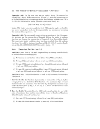
the same as for the Jaccard-distance family described in Section 3.6.2, except
the scale of distances is 0–180 rather than 0–1. That is, F is a
(d1 , d2 , (180 − d1 )/180, d2 /180)-sensitive
family of hash functions. From this basis, we can amplify the family as we wish,
just as for the minhash-based family.
3.7.3 Sketches
Instead of chosing a random vector from all possible vectors, it turns out to be
sufficiently random if we restrict our choice to vectors whose components are
+1 and −1. The dot product of any vector x with a vector v of +1’s and −1’s
is formed by adding the components of x where v is +1 and then subtracting
the other components of x – those where v is −1.
If we pick a collection of random vectors, say v1 , v2 , . . . , vn , then we can
apply them to an arbitrary vector x by computing v1 .x, v2 .x, . . . , vn .x and then
replacing any positive value by +1 and any negative value by −1. The result is
called the sketch of x. You can handle 0’s arbitrarily, e.g., by chosing a result +1
or −1 at random. Since there is only a tiny probability of a zero dot product,
the choice has essentially no effect.
Example 3.21 : Suppose our space consists of 4-dimensional vectors, and we
pick three random vectors: v1 = [+1, −1, +1, +1], v2 = [−1, +1, −1, +1], and
v3 = [+1, +1, −1, −1]. For the vector x = [3, 4, 5, 6], the sketch is [+1, +1, −1].
That is, v1 .x = 3−4+5+6 = 10. Since the result is positive, the first component
of the sketch is +1. Similarly, v2 .x = 3 and v3 .x = −4, so the second component
of the sketch is +1 and the third component is −1.
Consider the vector y = [4, 3, 2, 1]. We can similarly compute its sketch to
be [+1, −1, +1]. Since the sketches for x and y agree in 1/3 of the positions,
we estimate that the angle between them is 120 degrees. That is, a randomly
chosen hyperplane is twice as likely to look like the dashed line in Fig. 3.12 than
like the dotted line.
The above conclusion turns out to be quite wrong. We can calculate the
cosine of the angle between x and y to be x.y, which is
6 × 1 + 5 × 2 + 4 × 3 + 3 × 4 = 40
divided by the magnitudes of the two vectors. These magnitudes are
62 + 52 + 42 + 32 = 9.274
√
and 12 + 22 + 32 + 42 = 5.477. Thus, the cosine of the angle between x and
y is 0.7875, and this angle is about 38 degrees. However, if you look at all
16 different vectors v of length 4 that have +1 and −1 as components, you
find that there are only four of these whose dot products with x and y have
a different sign, namely v2 , v3 , and their complements [+1, −1, +1, −1] and
[−1, −1, +1, +1]. Thus, had we picked all sixteen of these vectors to form a
sketch, the estimate of the angle would have been 180/4 = 45 degrees. 2](https://image.slidesharecdn.com/miningofmassivedatasets-120805173332-phpapp01/85/Mining-of-massive-datasets-104-320.jpg)
![90 CHAPTER 3. FINDING SIMILAR ITEMS
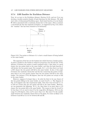
We conclude that the family F just described forms a (a/2, 2a, 1/2, 1/3)-
sensitive family of hash functions. That is, for distances up to a/2 the proba-
bility is at least 1/2 that two points at that distance will fall in the same bucket,
while for distances at least 2a the probability points at that distance will fall in
the same bucket is at most 1/3. We can amplify this family as we like, just as
for the other examples of locality-sensitive hash functions we have discussed.
3.7.5 More LSH Families for Euclidean Spaces
There is something unsatisfying about the family of hash functions developed
in Section 3.7.4. First, the technique was only described for two-dimensional
Euclidean spaces. What happens if our data is points in a space with many
dimensions? Second, for Jaccard and cosine distances, we were able to develop
locality-sensitive families for any pair of distances d1 and d2 as long as d1 < d2 .
In Section 3.7.4 we appear to need the stronger condition d1 < 4d2 .
However, we claim that there is a locality-sensitive family of hash func-
tions for any d1 < d2 and for any number of dimensions. The family’s hash
functions still derive from random lines through the space and a bucket size
a that partitions the line. We still hash points by projecting them onto the
line. Given that d1 < d2 , we may not know what the probability p1 is that two
points at distance d1 hash to the same bucket, but we can be certain that it
is greater than p2 , the probability that two points at distance d2 hash to the
same bucket. The reason is that this probability surely grows as the distance
shrinks. Thus, even if we cannot calculate p1 and p2 easily, we know that there
is a (d1 , d2 , p1 , p2 )-sensitive family of hash functions for any d1 < d2 and any
given number of dimensions.
Using the amplification techniques of Section 3.6.3, we can then adjust the
two probabilities to surround any particular value we like, and to be as far apart
as we like. Of course, the further apart we want the probabilities to be, the
larger the number of basic hash functions in F we must use.
3.7.6 Exercises for Section 3.7
Exercise 3.7.1 : Suppose we construct the basic family of six locality-sensitive
functions for vectors of length six. For each pair of the vectors 000000, 110011,
010101, and 011100, which of the six functions makes them candidates?
Exercise 3.7.2 : Let us compute sketches using the following four “random”
vectors:
v1 = [+1, +1, +1, −1] v2 = [+1, +1, −1, +1]
v3 = [+1, −1, +1, +1] v4 = [−1, +1, +1, +1]
Compute the sketches of the following vectors.
(a) [2, 3, 4, 5].](https://image.slidesharecdn.com/miningofmassivedatasets-120805173332-phpapp01/85/Mining-of-massive-datasets-106-320.jpg)
![3.8. APPLICATIONS OF LOCALITY-SENSITIVE HASHING 91
(b) [−2, 3, −4, 5].
(c) [2, −3, 4, −5].
For each pair, what is the estimated angle between them, according to the
sketches? What are the true angles?
Exercise 3.7.3 : Suppose we form sketches by using all sixteen of the vectors
of length 4, whose components are each +1 or −1. Compute the sketches of
the three vectors in Exercise 3.7.2. How do the estimates of the angles between
each pair compare with the true angles?
Exercise 3.7.4 : Suppose we form sketches using the four vectors from Exer-
cise 3.7.2.
! (a) What are the constraints on a, b, c, and d that will cause the sketch of
the vector [a, b, c, d] to be [+1, +1, +1, +1]?
!! (b) Consider two vectors [a, b, c, d] and [e, f, g, h]. What are the conditions on
a, b, . . . , h that will make the sketches of these two vectors be the same?
Exercise 3.7.5 : Suppose we have points in a 3-dimensional Euclidean space:
p1 = (1, 2, 3), p2 = (0, 2, 4), and p3 = (4, 3, 2). Consider the three hash functions
defined by the three axes (to make our calculations very easy). Let buckets be
of length a, with one bucket the interval [0, a) (i.e., the set of points x such that
0 ≤ x < a), the next [a, 2a), the previous one [−a, 0), and so on.
(a) For each of the three lines, assign each of the points to buckets, assuming
a = 1.
(b) Repeat part (a), assuming a = 2.
(c) What are the candidate pairs for the cases a = 1 and a = 2?
! (d) For each pair of points, for what values of a will that pair be a candidate
pair?
3.8 Applications of Locality-Sensitive Hashing
In this section, we shall explore three examples of how LSH is used in practice.
In each case, the techniques we have learned must be modified to meet certain
constraints of the problem. The three subjects we cover are:
1. Entity Resolution: This term refers to matching data records that refer to
the same real-world entity, e.g., the same person. The principal problem
addressed here is that the similarity of records does not match exactly
either the similar-sets or similar-vectors models of similarity on which the
theory is built.](https://image.slidesharecdn.com/miningofmassivedatasets-120805173332-phpapp01/85/Mining-of-massive-datasets-107-320.jpg)
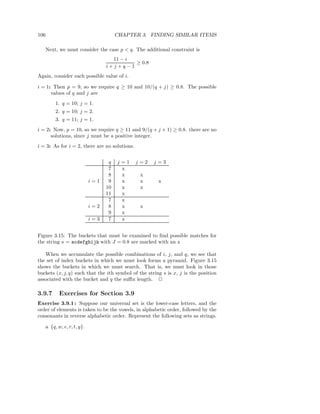
![110 CHAPTER 3. FINDING SIMILAR ITEMS
of the string times the maximum Jaccard distance (1 minus the minimum
Jaccard similarity).
3 Position Indexes: We can index strings not only on the characters in
their prefixes, but on the position of that character within the prefix. We
reduce the number of pairs of strings that must be compared, because
if two strings share a character that is not in the first position in both
strings, then we know that either there are some preceding characters that
are in the union but not the intersection, or there is an earlier symbol that
appears in both strings.
3 Suffix Indexes: We can also index strings based not only on the characters
in their prefixes and the positions of those characters, but on the length
of the character’s suffix – the number of positions that follow it in the
string. This structure further reduces the number of pairs that must be
compared, because a common symbol with different suffix lengths implies
additional characters that must be in the union but not in the intersection.
3.11 References for Chapter 3
The technique we called shingling is attributed to [10]. The use in the manner
we discussed here is from [2]. Minhashing comes from [3]. The original works
on locality-sensitive hashing were [9] and [7]. [1] is a useful summary of ideas
in this field.
[4] introduces the idea of using random-hyperplanes to summarize items in
a way that respects the cosine distance. [8] suggests that random hyperplanes
plus LSH can be more accurate at detecting similar documents than minhashing
plus LSH.
Techniques for summarizing points in a Euclidean space are covered in [6].
[11] presented the shingling technique based on stop words.
The length and prefix-based indexing schemes for high-similarity matching
comes from [5]. The technique involving suffix length is from [12].
1. A. Andoni and P. Indyk, “Near-optimal hashing algorithms for approxi-
mate nearest neighbor in high dimensions,” Comm. ACM 51:1, pp. 117–
122, 2008.
2. A.Z. Broder, “On the resemblance and containment of documents,” Proc.
Compression and Complexity of Sequences, pp. 21–29, Positano Italy,
1997.
3. A.Z. Broder, M. Charikar, A.M. Frieze, and M. Mitzenmacher, “Min-wise
independent permutations,” ACM Symposium on Theory of Computing,
pp. 327–336, 1998.
4. M.S. Charikar, “Similarity estimation techniques from rounding algo-
rithms,” ACM Symposium on Theory of Computing, pp. 380–388, 2002.](https://image.slidesharecdn.com/miningofmassivedatasets-120805173332-phpapp01/85/Mining-of-massive-datasets-126-320.jpg)

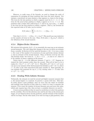
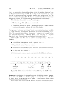
![4.9. REFERENCES FOR CHAPTER 4 143
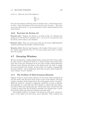
3 Estimating the Number of 1’s in a Window : We can estimate the number
of 1’s in a window of 0’s and 1’s by grouping the 1’s into buckets. Each
bucket has a number of 1’s that is a power of 2; there are one or two
buckets of each size, and sizes never decrease as we go back in time. If
we record only the position and size of the buckets, we can represent the
contents of a window of size N with O(log2 N ) space.
3 Answering Queries About Numbers of 1’s: If we want to know the approx-
imate numbers of 1’s in the most recent k elements of a binary stream,
we find the earliest bucket B that is at least partially within the last k
positions of the window and estimate the number of 1’s to be the sum of
the sizes of each of the more recent buckets plus half the size of B. This
estimate can never be off by more that 50% of the true count of 1’s.
3 Closer Approximations to the Number of 1’s: By changing the rule for
how many buckets of a given size can exist in the representation of a
binary window, so that either r or r − 1 of a given size may exist, we can
assure that the approximation to the true number of 1’s is never off by
more than 1/r.
3 Exponentially Decaying Windows: Rather than fixing a window size, we
can imagine that the window consists of all the elements that ever arrived
in the stream, but with the element that arrived t time units ago weighted
by e−ct for some time-constant c. Doing so allows us to maintain certain
summaries of an exponentially decaying window easily. For instance, the
weighted sum of elements can be recomputed, when a new element arrives,
by multiplying the old sum by 1 − c and then adding the new element.
3 Maintaining Frequent Elements in an Exponentially Decaying Window :
We can imagine that each item is represented by a binary stream, where
0 means the item was not the element arriving at a given time, and 1
means that it was. We can find the elements whose sum of their binary
stream is at least 1/2. When a new element arrives, multiply all recorded
sums by 1 minus the time constant, add 1 to the count of the item that
just arrived, and delete from the record any item whose sum has fallen
below 1/2.
4.9 References for Chapter 4
Many ideas associated with stream management appear in the “chronicle data
model” of [8]. An early survey of research in stream-management systems is
[2]. Also, [6] is a recent book on the subject of stream management.
The sampling technique of Section 4.2 is from [7]. The Bloom Filter is
generally attributed to [3], although essentially the same technique appeared as
“superimposed codes” in [9].](https://image.slidesharecdn.com/miningofmassivedatasets-120805173332-phpapp01/85/Mining-of-massive-datasets-159-320.jpg)
![144 CHAPTER 4. MINING DATA STREAMS
The algorithm for counting distinct elements is essentially that of [5], al-
though the particular method we described appears in [1]. The latter is also
the source for the algorithm for calculating the surprise number and higher
moments. However, the technique for maintaining a uniformly chosen sample
of positions in the stream is called “reservoir sampling” and comes from [10].
The technique for approximately counting 1’s in a window is from [4].
1. N. Alon, Y. Matias, and M. Szegedy, “The space complexity of approxi-
mating frequency moments,” 28th ACM Symposium on Theory of Com-
puting, pp. 20–29, 1996.
2. B. Babcock, S. Babu, M. Datar, R. Motwani, and J. Widom, “Models
and issues in data stream systems,” Symposium on Principles of Database
Systems, pp. 1–16, 2002.
3. B.H. Bloom, “Space/time trade-offs in hash coding with allowable errors,”
Comm. ACM 13:7, pp. 422–426, 1970.
4. M. Datar, A. Gionis, P. Indyk, and R. Motwani, “Maintaining stream
statistics over sliding windows,” SIAM J. Computing 31, pp. 1794–1813,
2002.
5. P. Flajolet and G.N. Martin, “Probabilistic counting for database applica-
tions,” 24th Symposium on Foundations of Computer Science, pp. 76–82,
1983.
6. M. Garofalakis, J. Gehrke, and R. Rastogi (editors), Data Stream Man-
agement, Springer, 2009.
7. P.B. Gibbons, “Distinct sampling for highly-accurate answers to distinct
values queries and event reports,” Intl. Conf. on Very Large Databases,
pp. 541–550, 2001.
8. H.V. Jagadish, I.S. Mumick, and A. Silberschatz, “View maintenance
issues for the chronicle data model,” Proc. ACM Symp. on Principles of
Database Systems, pp. 113–124, 1995.
9. W.H. Kautz and R.C. Singleton, “Nonadaptive binary superimposed codes,”
IEEE Transactions on Information Theory 10, pp. 363–377, 1964.
10. J. Vitter, “Random sampling with a reservoir,” ACM Transactions on
Mathematical Software 11:1, pp. 37–57, 1985.](https://image.slidesharecdn.com/miningofmassivedatasets-120805173332-phpapp01/85/Mining-of-massive-datasets-160-320.jpg)
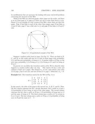
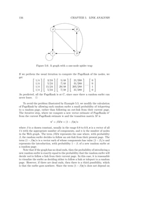
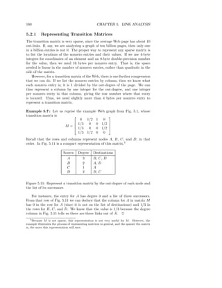
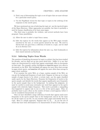
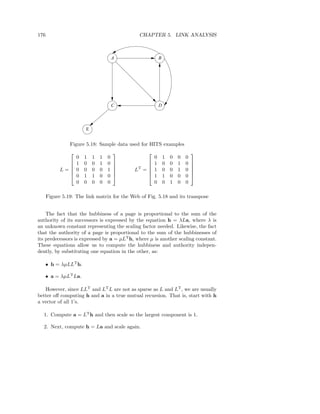
![182 CHAPTER 5. LINK ANALYSIS
HITS equations in the way they do for PageRank, so no taxation scheme
is necessary.
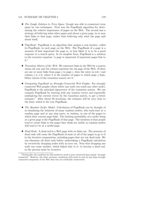
5.7 References for Chapter 5
The PageRank algorithm was first expressed in [1]. The experiments on the
structure of the Web, which we used to justify the existence of dead ends and
spider traps, were described in [2]. The block-stripe method for performing the
PageRank iteration is taken from [5].
Topic-sensitive PageRank is taken from [6]. TrustRank is described in [4],
and the idea of spam mass is taken from [3].
The HITS (hubs and authorities) idea was described in [7].
1. S. Brin and L. Page, “Anatomy of a large-scale hypertextual web search
engine,” Proc. 7th Intl. World-Wide-Web Conference, pp. 107–117, 1998.
2. A. Broder, R. Kumar, F. Maghoul, P. Raghavan, S. Rajagopalan, R.
Stata, A. Tomkins, and J. Weiner, “Graph structure in the web,” Com-
puter Networks 33:1–6, pp. 309–320, 2000.
3. Z. Gy¨ngi, P. Berkhin, H. Garcia-Molina, and J. Pedersen, “Link spam
o
detection based on mass estimation,” Proc. 32nd Intl. Conf. on Very Large
Databases, pp. 439–450, 2006.
4. Z. Gy¨ngi, H. Garcia-Molina, and J. Pedersen, “Combating link spam
o
with trustrank,” Proc. 30th Intl. Conf. on Very Large Databases, pp. 576–
587, 2004.
5. T.H. Haveliwala, “Efficient computation of PageRank,” Stanford Univ.
Dept. of Computer Science technical report, Sept., 1999. Available as
http://infolab.stanford.edu/~taherh/papers/efficient-pr.pdf
6. T.H. Haveliwala, “Topic-sensitive PageRank,” Proc. 11th Intl. World-
Wide-Web Conference, pp. 517–526, 2002
7. J.M. Kleinberg, “Authoritative sources in a hyperlinked environment,” J.
ACM 46:5, pp. 604–632, 1999.](https://image.slidesharecdn.com/miningofmassivedatasets-120805173332-phpapp01/85/Mining-of-massive-datasets-198-320.jpg)
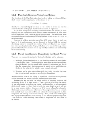
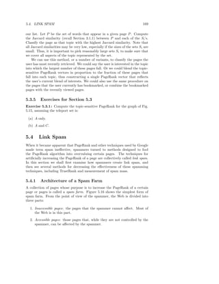
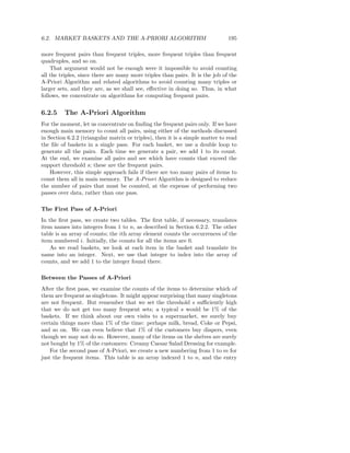
![192 CHAPTER 6. FREQUENT ITEMSETS
Moreover, all the algorithms we discuss have the property that they read the
basket file sequentially. Thus, algorithms can be characterized by the number
of passes through the basket file that they make, and their running time is
proportional to the product of the number of passes they make through the
basket file times the size of that file. Since we cannot control the amount of
data, only the number of passes taken by the algorithm matters, and it is that
aspect of the algorithm that we shall focus upon when measuring the running
time of a frequent-itemset algorithm.
6.2.2 Use of Main Memory for Itemset Counting
There is a second data-related issue that we must examine, however. All
frequent-itemset algorithms require us to maintain many different counts as
we make a pass through the data. For example, we might need to count the
number of times that each pair of items occurs in baskets. If we do not have
enough main memory to store each of the counts, then adding 1 to a random
count will most likely require us to load a page from disk. In that case, the
algorithm will thrash and run many orders of magnitude slower than if we were
certain to find each count in main memory. The conclusion is that we cannot
count anything that doesn’t fit in main memory. Thus, each algorithm has a
limit on how many items it can deal with.
Example 6.5 : Suppose a certain algorithm has to count all pairs of items,
and there are n items. We thus need space to store n integers, or about
2
n2 /2 integers. If integers take 4 bytes, we require 2n2 bytes. If our machine
has 2 gigabytes, or 231 bytes of main memory, then we require n ≤ 215 , or
approximately n < 33,000. 2
It is not trivial to store the n counts in a way that makes it easy to find
2
the count for a pair {i, j}. First, we have not assumed anything about how
items are represented. They might, for instance, be strings like “bread.” It
is more space-efficient to represent items by consecutive integers from 1 to n,
where n is the number of distinct items. Unless items are already represented
this way, we need a hash table that translates items as they appear in the file
to integers. That is, each time we see an item in the file, we hash it. If it is
already in the hash table, we can obtain its integer code from its entry in the
table. If the item is not there, we assign it the next available number (from a
count of the number of distinct items seen so far) and enter the item and its
code into the table.
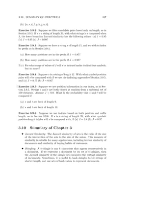
The Triangular-Matrix Method
Even after coding items as integers, we still have the problem that we must
count a pair {i, j} in only one place. For example, we could order the pair so
that i < j, and only use the entry a[i, j] in a two-dimensional array a. That
strategy would make half the array useless. A more space-efficient way is to](https://image.slidesharecdn.com/miningofmassivedatasets-120805173332-phpapp01/85/Mining-of-massive-datasets-208-320.jpg)
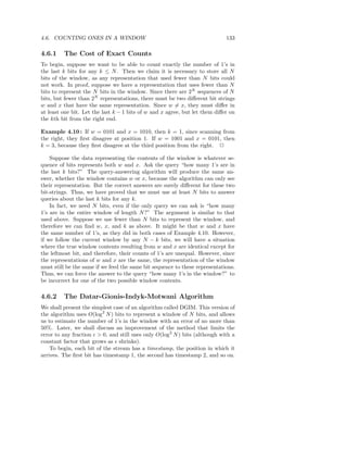
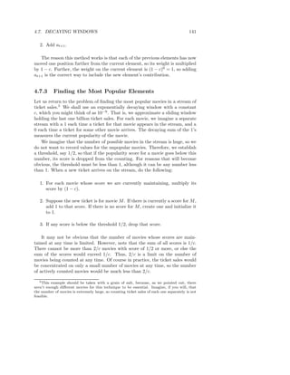
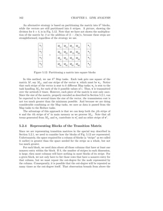
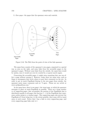
![6.2. MARKET BASKETS AND THE A-PRIORI ALGORITHM 193
use a one-dimensional triangular array. We store in a[k] the count for the pair
{i, j}, with 1 ≤ i < j ≤ n, where
i
k = (i − 1) n − +j−i
2
The result of this layout is that the pairs are stored in lexicographic order, that
is first {1, 2}, {1, 3}, . . . , {1, n}, then {2, 3}, {2, 4}, . . . , {2, n}, and so on, down
to {n − 2, n − 1}, {n − 2, n}, and finally {n − 1, n}.
The Triples Method
There is another approach to storing counts that may be more appropriate,
depending on the fraction of the possible pairs of items that actually appear in
some basket. We can store counts as triples [i, j, c], meaning that the count of
pair {i, j}, with i < j, is c. A data structure, such as a hash table with i and
j as the search key, is used so we can tell if there is a triple for a given i and j
and, if so, to find it quickly. We call this approach the triples method of storing
counts.
Unlike the triangular matrix, the triples method does not require us to store
anything if the count for a pair is 0. On the other hand, the triples method
requires us to store three integers, rather than one, for every pair that does
appear in some basket. In addition, there is the space needed for the hash
table or other data structure used to support efficient retrieval. The conclusion
is that the triangular matrix will be better if at least 1/3 of the n possible
2
pairs actually appear in some basket, while if significantly fewer than 1/3 of the
possible pairs occur, we should consider using the triples method.
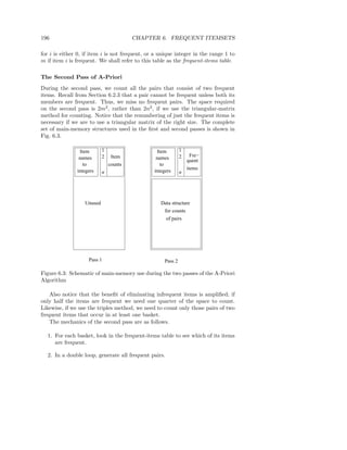
Example 6.6 : Suppose there are 100,000 items, and 10,000,000 baskets of 10
items each. Then the triangular-matrix method requires 100000 = 5 × 10⁹
2
(approximately) integer counts.1 On the other hand, the total number of pairs
among all the baskets is 107 10 = 4.5 × 10⁸ . Even in the extreme case that
2
every pair of items appeared only once, there could be only 4.5 × 10⁸ pairs with
nonzero counts. If we used the triples method to store counts, we would need
only three times that number of integers, or 1.35 × 10⁹ integers. Thus, in this
case the triples method will surely take much less space than the triangular
matrix.
However, even if there were ten or a hundred times as many baskets, it
would be normal for there to be a sufficiently uneven distribution of items that
we might still be better off using the triples method. That is, some pairs would
have very high counts, and the number of different pairs that occurred in one
or more baskets would be much less than the theoretical maximum number of
such pairs. 2
1 Here,
`n´
and throughout the chapter, we shall use the approximation that 2
= n2 /2 for
large n.](https://image.slidesharecdn.com/miningofmassivedatasets-120805173332-phpapp01/85/Mining-of-massive-datasets-209-320.jpg)
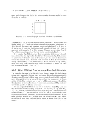
![198 CHAPTER 6. FREQUENT ITEMSETS
in Section 6.2.4 implies that there will not be too many frequent pairs, so they
can be listed in a main-memory table. Likewise, there will not be too many
candidate triples, so these can all be counted by a generalization of the triples
method. That is, while triples are used to count pairs, we would use quadruples,
consisting of the three item codes and the associated count, when we want to
count triples. Similarly, we can count sets of size k using tuples with k + 1
components, the last of which is the count, and the first k of which are the item
codes, in sorted order.
To find L3 we make a third pass through the basket file. For each basket,
we need only look at those items that are in L1 . From these items, we can
examine each pair and determine whether or not that pair is in L2 . Any item
of the basket that does not appear in at least two frequent pairs, both of which
consist of items in the basket, cannot be part of a frequent triple that the
basket contains. Thus, we have a fairly limited search for triples that are both
contained in the basket and are candidates in C3 . Any such triples found have
1 added to their count.
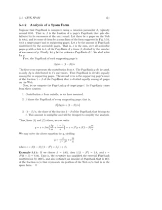
Example 6.8 : Suppose our basket consists of items 1 through 10. Of these, 1
through 5 have been found to be frequent items, and the following pairs have
been found frequent: {1, 2}, {2, 3}, {3, 4}, and {4, 5}. At first, we eliminate the
nonfrequent items, leaving only 1 through 5. However, 1 and 5 appear in only
one frequent pair in the itemset, and therefore cannot contribute to a frequent
triple contained in the basket. Thus, we must consider adding to the count of
triples that are contained in {2, 3, 4}. There is only one such triple, of course.
However, we shall not find it in C3 , because {2, 4} evidently is not frequent. 2
The construction of the collections of larger frequent itemsets and candidates
proceeds in essentially the same manner, until at some pass we find no new
frequent itemsets and stop. That is:
1. Define Ck to be all those itemsets of size k, every k − 1 of which is an
itemset in Lk−1 .
2. Find Lk by making a pass through the baskets and counting all and only
the itemsets of size k that are in Ck . Those itemsets that have count at
least s are in Lk .
6.2.7 Exercises for Section 6.2
Exercise 6.2.1 : If we use a triangular matrix to count pairs, and n, the num-
ber of items, is 20, what pair’s count is in a[100]?
! Exercise 6.2.2 : In our description of the triangular-matrix method in Sec-
tion 6.2.2, the formula for k involves dividing an arbitrary integer i by 2. Yet
we need to have k always be an integer. Prove that k will, in fact, be an integer.](https://image.slidesharecdn.com/miningofmassivedatasets-120805173332-phpapp01/85/Mining-of-massive-datasets-214-320.jpg)

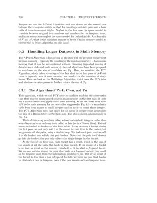
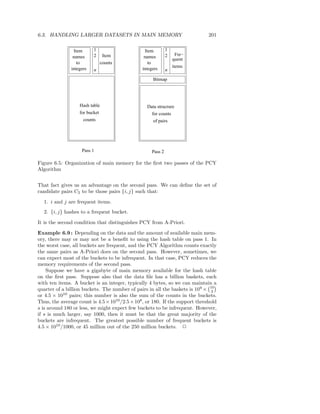
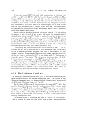
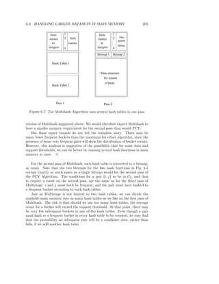
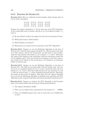
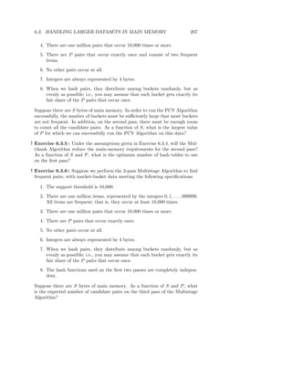
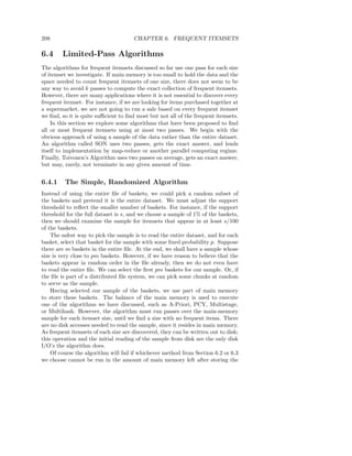
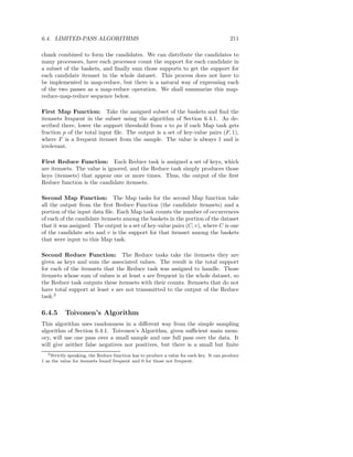
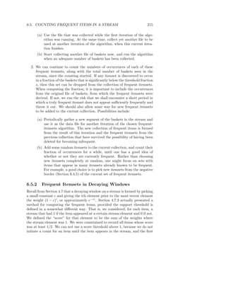
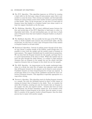
![220 CHAPTER 6. FREQUENT ITEMSETS
3 Frequent Itemsets in Streams: If we use a decaying window with constant
c, then we can start counting an item whenever we see it in a basket. We
start counting an itemset if we see it contained within the current basket,
and all its immediate proper subsets already are being counted. As the
window is decaying, we multiply all counts by 1 − c and eliminate those
that are less than 1/2.
6.7 References for Chapter 6
The market-basket data model, including association rules and the A-Priori
Algorithm, are from [1] and [2].
The PCY Algorithm is from [4]. The Multistage and Multihash Algorithms
are found in [3].
The SON Algorithm is from [5]. Toivonen’s Algorithm appears in [6].
1. R. Agrawal, T. Imielinski, and A. Swami, “Mining associations between
sets of items in massive databases,” Proc. ACM SIGMOD Intl. Conf. on
Management of Data, pp. 207–216, 1993.
2. R. Agrawal and R. Srikant, “Fast algorithms for mining association rules,”
Intl. Conf. on Very Large Databases, pp. 487–499, 1994.
3. M. Fang, N. Shivakumar, H. Garcia-Molina, R. Motwani, and J.D. Ull-
man, “Computing iceberg queries efficiently,” Intl. Conf. on Very Large
Databases, pp. 299-310, 1998.
4. J.S. Park, M.-S. Chen, and P.S. Yu, “An effective hash-based algorithm
for mining association rules,” Proc. ACM SIGMOD Intl. Conf. on Man-
agement of Data, pp. 175–186, 1995.
5. A. Savasere, E. Omiecinski, and S.B. Navathe, “An efficient algorithm for
mining association rules in large databases,” Intl. Conf. on Very Large
Databases, pp. 432–444, 1995.
6. H. Toivonen, “Sampling large databases for association rules,” Intl. Conf.
on Very Large Databases, pp. 134–145, 1996.](https://image.slidesharecdn.com/miningofmassivedatasets-120805173332-phpapp01/85/Mining-of-massive-datasets-236-320.jpg)
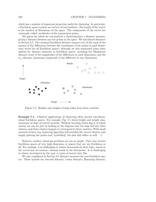
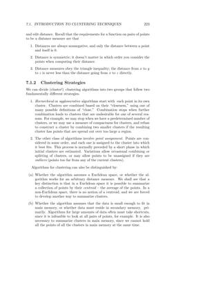
![224 CHAPTER 7. CLUSTERING
7.1.3 The Curse of Dimensionality
High-dimensional Euclidean spaces have a number of unintuitive properties that
are sometimes referred to as the “curse of dimensionality.” Non-Euclidean
spaces usually share these anomalies as well. One manifestation of the “curse”
is that in high dimensions, almost all pairs of points are equally far away from
one another. Another manifestation is that almost any two vectors are almost
orthogonal. We shall explore each of these in turn.
The Distribution of Distances in a High-Dimensional Space
Let us consider a d-dimensional Euclidean space. Suppose we choose n random
points in the unit cube, i.e., points [x1 , x2 , . . . , xd ], where each xi is in the range
0 to 1. If d = 1, we are placing random points on a line of length 1. We expect
that some pairs of points will be very close, e.g., consecutive points on the
line. We also expect that some points will be very far away – those at or near
opposite ends of the line. The average distance between a pair of points is 1/3.1
Suppose that d is very large. The Euclidean distance between two random
points [x1 , x2 , . . . , xd ] and [y1 , y2 , . . . , yd ] is
d
(xi − yi )2
i=1
Here, each xi and yi is a random variable chosen uniformly in the range 0 to
1. Since d is large, we can expect that for some i, |xi − yi | will be close to 1.
That puts a lower bound of 1 on the distance between almost any two random
points. In fact, a more careful argument can put a stronger lower bound on
the distance between all but a vanishingly small fraction of the pairs of points.
√
However, the maximum distance between two points is d, and one can argue
that all but a vanishingly small fraction of the pairs do not have a distance
close to this upper limit. In fact, almost all points will have a distance close to
the average distance.
If there are essentially no pairs of points that are close, it is hard to build
clusters at all. There is little justification for grouping one pair of points and
not another. Of course, the data may not be random, and there may be useful
clusters, even in very high-dimensional spaces. However, the argument about
random data suggests that it will be hard to find these clusters among so many
pairs that are all at approximately the same distance.
Angles Between Vectors
Suppose again that we have three random points A, B, and C in a d-dimensional
space, where d is large. Here, we do not assume points are in the unit cube;
1 You can prove this fact by evaluating a double integral, but we shall not do the math
here, as it is not central to the discussion.](https://image.slidesharecdn.com/miningofmassivedatasets-120805173332-phpapp01/85/Mining-of-massive-datasets-240-320.jpg)
![7.2. HIERARCHICAL CLUSTERING 225
they can be anywhere in the space. What is angle ABC? We may assume that
A is the point [x1 , x2 , . . . , xd ] and C is the point [y1 , y2 , . . . , yd ], while B is the
origin. Recall from Section 3.5.4 that the cosine of the angle ABC is the dot
product of A and C divided by the product of the lengths of the vectors A and
C. That is, the cosine is
d
i=0 xi yi
d d
i=1 x2
i i=1
2
yi
As d grows, the denominator grows linearly in d, but the numerator is a sum
of random values, which are as likely to be positive as negative. Thus, the
expected value√ the numerator is 0, and as d grows, its standard deviation
of
grows only as d. Thus, for large d, the cosine of the angle between any two
vectors is almost certain to be close to 0, which means the angle is close to 90
degrees.
An important consequence of random vectors being orthogonal is that if we
have three random points A, B, and C, and we know the distance from A to B
is d1 , while the distance from B to C is d2 , we can assume the distance from A
to C is approximately d2 + d2 . That rule does not hold, even approximately,
1 2
if the number of dimensions is small. As an extreme case, if d = 1, then the
distance from A to C would necessarily be d1 + d2 if A and C were on opposite
sides of B, or |d1 − d2 | if they were on the same side.
7.1.4 Exercises for Section 7.1
! Exercise 7.1.1 : Prove that if you choose two points uniformly and indepen-
dently on a line of length 1, then the expected distance between the points is
1/3.
!! Exercise 7.1.2 : If you choose two points uniformly in the unit square, what
is their expected Eclidean distance?
! Exercise 7.1.3 : Suppose we have a d-dimensional Euclidean space. Consider
vectors whose components are only +1 or −1 in each dimension. Note that
√
each vector has length d, so the product of their lengths (denominator in
the formula for the cosine of the angle between them) is d. If we chose each
component independently, and a component is as likely to be +1 as −1, what
is the distribution of the value of the numerator of the formula (i.e., the sum
of the products of the corresponding components from each vector)? What can
you say about the expected value of the cosine of the angle between the vectors,
as d grows large?
7.2 Hierarchical Clustering
We begin by considering hierarchical clustering in a Euclidean space. This
algorithm can only be used for relatively small datasets, but even so, there](https://image.slidesharecdn.com/miningofmassivedatasets-120805173332-phpapp01/85/Mining-of-massive-datasets-241-320.jpg)
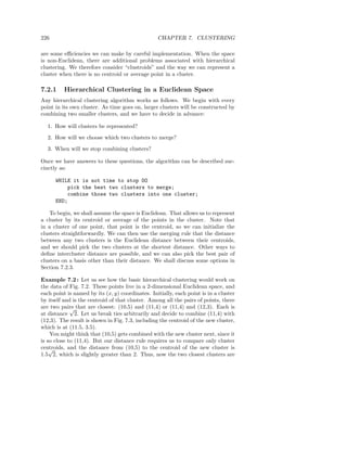
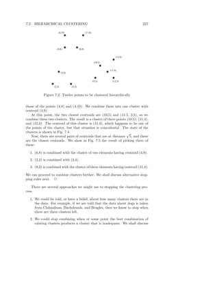
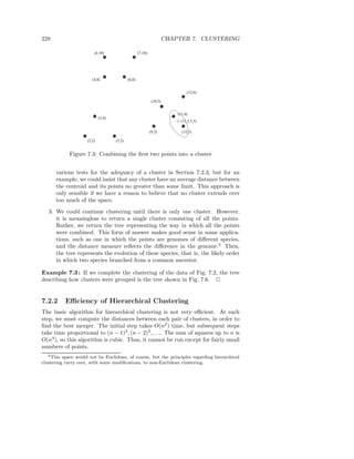
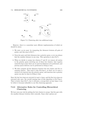
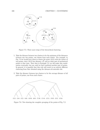
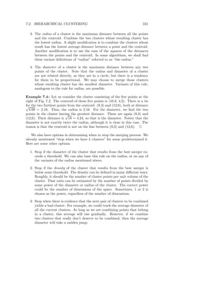
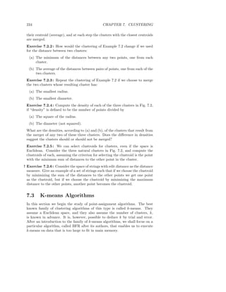
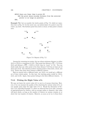
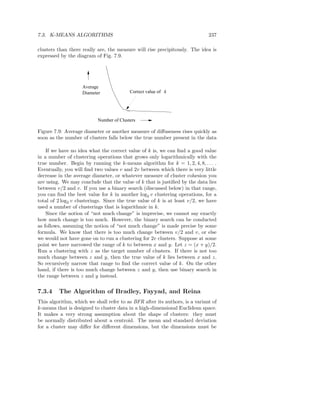
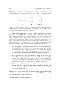
![7.3. K-MEANS ALGORITHMS 239
Points in the
retained set
Compressed sets
Its centroid
A cluster. Its points
are in the discard set.
Figure 7.11: Points in the discard, compressed, and retained sets
(b) The sum of the components of all the points in each dimension. This data
is a vector SUM of length d, and the component in the ith dimension is
SUMi .
(c) The sum of the squares of the components of all the points in each di-
mension. This data is a vector SUMSQ of length d, and its component in
the ith dimension is SUMSQi .
Our real goal is to represent a set of points by their count, their centroid and
the standard deviation in each dimension. However, these 2d + 1 values give us
those statistics. N is the count. The centroid’s coordinate in the ith dimension
is the SUMi /N , that is the sum in that dimension divided by the number of
points. The variance in the ith dimension is SUMSQi /N − (SUMi /N )2 . We can
compute the standard deviation in each dimension, since it is the square root
of the variance.
Example 7.9 : Suppose a cluster consists of the points (5, 1), (6, −2), and
(7, 0). Then N = 3, SUM = [18, −1], and SUMSQ = [110, 5]. The centroid is
SUM/N , or [6, −1/3]. The variance in the first dimension is 110/3 − (18/3)2 =
√
0.667, so the standard deviation is 0.667 = 0.816. In the second dimension,
the variance is 5/3 − (−1/3)2 = 1.56, so the standard deviation is 1.25. 2
7.3.5 Processing Data in the BFR Algorithm
We shall now outline what happens when we process a chunk of points.](https://image.slidesharecdn.com/miningofmassivedatasets-120805173332-phpapp01/85/Mining-of-massive-datasets-255-320.jpg)
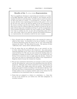
![7.3. K-MEANS ALGORITHMS 241
Finally, if this is the last chunk of input data, we need to do something
with the compressed and retained sets. We can treat them as outliers, and
never cluster them at all. Or, we can assign each point in the retained set to
the cluster of the nearest centroid. We can combine each minicluster with the
cluster whose centroid is closest to the centroid of the minicluster.
An important decision that must be examined is how we decide whether a
new point p is close enough to one of the k clusters that it makes sense to add
p to the cluster. Two approaches have been suggested.
(a) Add p to a cluster if it not only has the centroid closest to p, but it is
very unlikely that, after all the points have been processed, some other
cluster centroid will be found to be nearer to p. This decision is a complex
statistical calculation. It must assume that points are ordered randomly,
and that we know how many points will be processed in the future. Its
advantage is that if we find one centroid to be significantly closer to p
than any other, we can add p to that cluster and be done with it, even if
p is very far from all centroids.
(b) We can measure the probability that, if p belongs to a cluster, it would
be found as far as it is from the centroid of that cluster. This calculation
makes use of the fact that we believe each cluster to consist of normally
distributed points with the axes of the distribution aligned with the axes
of the space. It allows us to make the calculation through the Mahalanobis
distance of the point, which we shall describe next.
The Mahalanobis distance is essentially the distance between a point and
the centroid of a cluster, normalized by the standard deviation of the cluster
in each dimension. Since the BFR Algorithm assumes the axes of the cluster
align with the axes of the space, the computation of Mahalanobis distance is
especially simple. Let p = [p1 , p2 , . . . , pd ] be a point and c = [c1 , c2 , . . . , cd ] the
centroid of a cluster. Let σi be the standard deviation of points in the cluster
in the ith dimension. Then the Mahalanobis distance between p and c is
d
p i − ci 2
i=1
σi
That is, we normalize the difference between p and c in the ith dimension by
dividing by the standard deviation of the cluster in that dimension. The rest of
the formula combines the normalized distances in each dimension in the normal
way for a Euclidean space.
To assign point p to a cluster, we compute the Mahalanobis distance between
p and each of the cluster centroids. We choose that cluster whose centroid has
the least Mahalanobis distance, and we add p to that cluster provided the
Mahalanobis distance is less than a threshold. For instance, suppose we pick
four as the threshold. If data is normally distributed, then the probability of](https://image.slidesharecdn.com/miningofmassivedatasets-120805173332-phpapp01/85/Mining-of-massive-datasets-257-320.jpg)
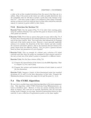
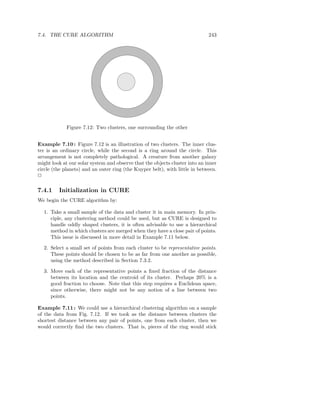
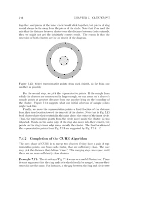
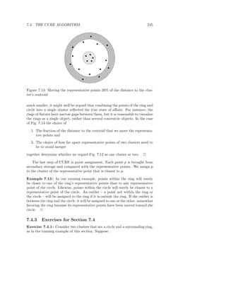
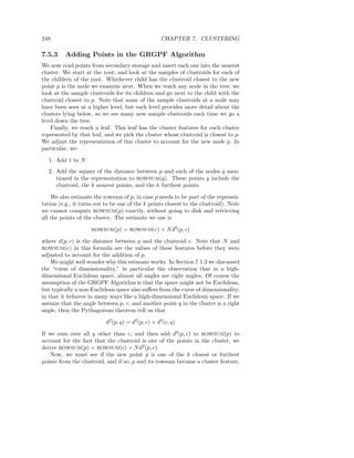
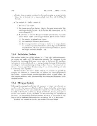
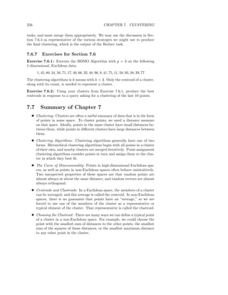
![260 CHAPTER 7. CLUSTERING
7.8 References for Chapter 7
The ancestral study of clustering for large-scale data is the BIRCH Algorithm
of [6]. The BFR Algorithm is from [2]. The CURE Algorithm is found in [5].
The paper on the GRGPF Algorithm is [3]. The necessary background
regarding B-trees and R-trees can be found in [4]. The study of clustering on
streams is taken from [1].
1. B. Babcock, M. Datar, R. Motwani, and L. O’Callaghan, “Maintaining
variance and k-medians over data stream windows,” Proc. ACM Symp.
on Principles of Database Systems, pp. 234–243, 2003.
2. P.S. Bradley, U.M. Fayyad, and C. Reina, “Scaling clustering algorithms
to large databases,” Proc. Knowledge Discovery and Data Mining, pp. 9–
15, 1998.
3. V. Ganti, R. Ramakrishnan, J. Gehrke, A.L. Powell, and J.C. French:,
“Clustering large datasets in arbitrary metric spaces,” Proc. Intl. Conf.
on Data Engineering, pp. 502–511, 1999.
4. H. Garcia-Molina, J.D. Ullman, and J. Widom, Database Systems: The
Complete Book Second Edition, Prentice-Hall, Upper Saddle River, NJ,
2009.
5. S. Guha, R. Rastogi, and K. Shim, “CURE: An efficient clustering algo-
rithm for large databases,” Proc. ACM SIGMOD Intl. Conf. on Manage-
ment of Data, pp. 73–84, 1998.
6. T. Zhang, R. Ramakrishnan, and M. Livny, “BIRCH: an efficient data
clustering method for very large databases,” Proc. ACM SIGMOD Intl.
Conf. on Management of Data, pp. 103–114, 1996.](https://image.slidesharecdn.com/miningofmassivedatasets-120805173332-phpapp01/85/Mining-of-massive-datasets-276-320.jpg)

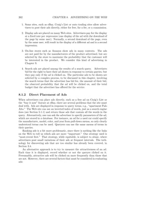

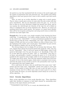
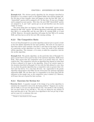
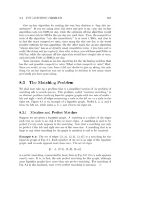
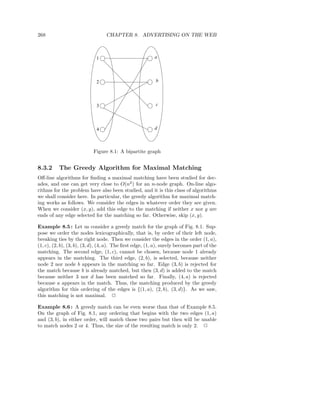
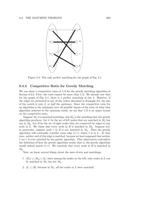
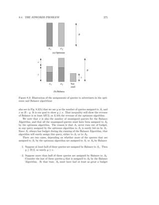
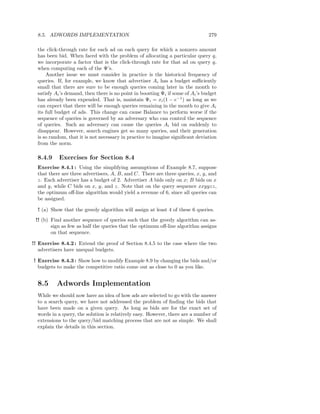
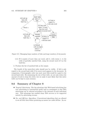
![8.7. REFERENCES FOR CHAPTER 8 285
3 The Balance Algorithm: This algorithm improves on the simple greedy
algorithm. A query’s ad is given to the advertiser who has bid on the query
and has the largest remaining budget. Ties can be broken arbitrarily.
3 Competitive Ratio of the Balance Algorithm: For the simplified adwords
model, the competitive ratio of the Balance Algorithm is 3/4 for the case
of two advertisers and 1−1/e, or about 63% for any number of advertisers.
3 The Balance Algorithm for the Generalized Adwords Problem: When bid-
ders can make differing bids, have different budgets, and have different
click-through rates for different queries, the Balance Algorithm awards an
ad to the advertiser with the highest value of the function Ψ = x(1−e−f ).
Here, x is the product of the bid and the click-through rate for that ad-
vertiser and query, and f is the fraction of the advertiser’s budget that
remains unspent.
3 Implementing an Adwords Algorithm: The simplest version of the imple-
mentation serves in situations where the bids are on exactly the set of
words in the search query. We can represent a query by the list of its
words, in sorted order. Bids are stored in a hash table or similar struc-
ture, with a hash key equal to the sorted list of words. A search query can
then be matched against bids by a straightforward lookup in the table.
3 Matching Word Sets Against Documents: A harder version of the ad-
words-implementation problem allows bids, which are still small sets of
words as in a search query, to be matched against larger documents, such
as emails or tweets. A bid set matches the document if all the words
appear in the document, in any order and not necessarily adjacent.
3 Hash Storage of Word Sets: A useful data structure stores the words of
each bid set in the order rarest-first. Documents have their words sorted
in the same order. Word sets are stored in a hash table with the first
word, in the rarest-first order, as the key.
3 Processing Documents for Bid Matches: We process the words of the
document rarest-first. Word sets whose first word is the current word
are copied to a temporary hash table, with the second word as the key.
Sets already in the temporary hash table are examined to see if the word
that is their key matches the current word, and, if so, they are rehashed
using their next word. Sets whose last word is matched are copied to the
output.
8.7 References for Chapter 8
[1] is an investigation of the way ad position influences the click-through rate.
The Balance Algorithm was developed in [2] and its application to the ad-
words problem is from [3].](https://image.slidesharecdn.com/miningofmassivedatasets-120805173332-phpapp01/85/Mining-of-massive-datasets-301-320.jpg)


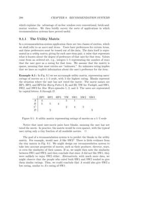
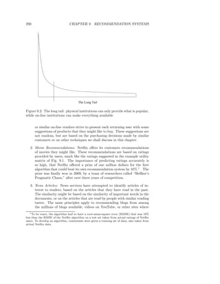
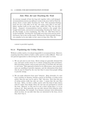
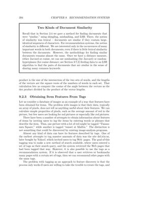
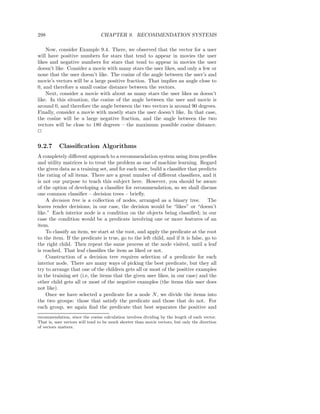
![300 CHAPTER 9. RECOMMENDATION SYSTEMS
Suppose that the group of articles that do not satisfy the predicate includes
sufficiently few positive examples that we can conclude all of these items are in
the “don’t-like” class. We may then put a leaf with decision “don’t like” as the
right child of the root. However, the articles that satisfy the predicate includes
a number of articles that user U doesn’t like; these are the articles that mention
the Yankees. Thus, at the left child of the root, we build another predicate.
We might find that the predicate “Yankees” OR “Jeter” OR “Teixeira” is the
best possible indicator of an article about baseball and about the Yankees.
Thus, we see in Fig. 9.3 the left child of the root, which applies this predicate.
Both children of this node are leaves, since we may suppose that the items
satisfying this predicate are predominantly negative and those not satisfying it
are predominantly positive. 2
Unfortunately, classifiers of all types tend to take a long time to construct.
For instance, if we wish to use decision trees, we need one tree per user. Con-
structing a tree not only requires that we look at all the item profiles, but we
have to consider many different predicates, which could involve complex com-
binations of features. Thus, this approach tends to be used only for relatively
small problem sizes.
9.2.8 Exercises for Section 9.2
Exercise 9.2.1 : Three computers, A, B, and C, have the numerical features
listed below:
Feature A B C
Processor Speed 3.06 2.68 2.92
Disk Size 500 320 640
Main-Memory Size 6 4 6
We may imagine these values as defining a vector for each computer; for in-
stance, A’s vector is [3.06, 500, 6]. We can compute the cosine distance between
any two of the vectors, but if we do not scale the components, then the disk
size will dominate and make differences in the other components essentially in-
visible. Let us use 1 as the scale factor for processor speed, α for the disk size,
and β for the main memory size.
(a) In terms of α and β, compute the cosines of the angles between the vectors
for each pair of the three computers.
(b) What are the angles between the vectors if α = β = 1?
(c) What are the angles between the vectors if α = 0.01 and β = 0.5?
! (d) One fair way of selecting scale factors is to make each inversely propor-
tional to the average value in its component. What would be the values
of α and β, and what would be the angles between the vectors?](https://image.slidesharecdn.com/miningofmassivedatasets-120805173332-phpapp01/85/Mining-of-massive-datasets-316-320.jpg)
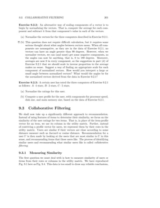
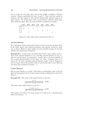
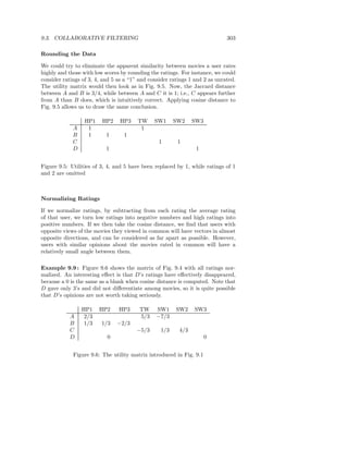
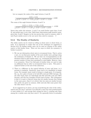
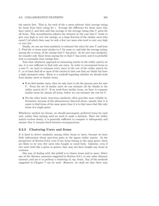
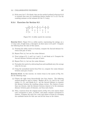
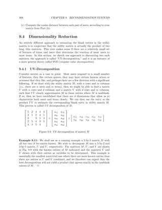
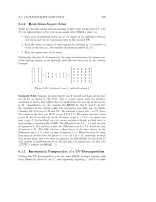
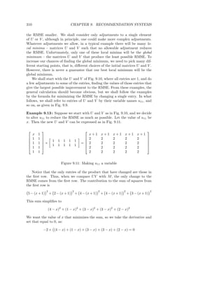
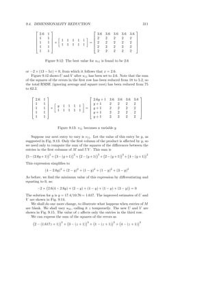
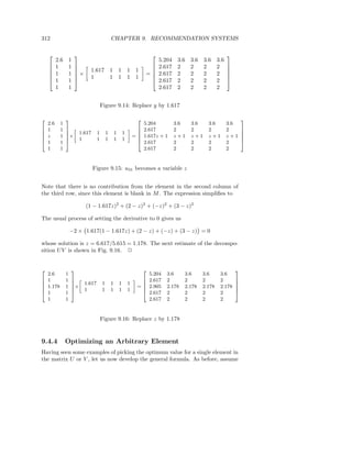
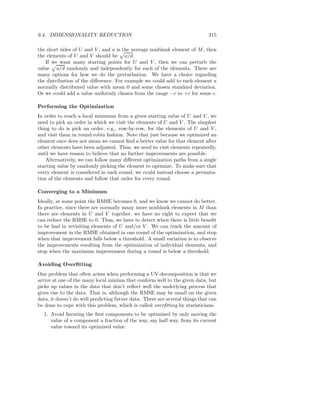
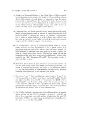
![320 CHAPTER 9. RECOMMENDATION SYSTEMS
9.7 References for Chapter 9
[1] is a survey of recommendation systems as of 2005. The argument regard-
ing the importance of the long tail in on-line systems is from [2], which was
expanded into a book [3].
[8] discusses the use of computer games to extract tags for items.
See [5] for a discussion of item-item similarity and how Amazon designed
its collaborative-filtering algorithm for product recommendations.
There are three papers describing the three algorithms that, in combination,
won the NetFlix challenge. They are [4], [6], and [7].
1. G. Adomavicius and A. Tuzhilin, “Towards the next generation of rec-
ommender systems: a survey of the state-of-the-art and possible exten-
sions,” IEEE Trans. on Data and Knowledge Engineering 17:6, pp. 734–
749, 2005.
2. C. Anderson,
http://www.wired.com/wired/archive/12.10/tail.html
2004.
3. C. Anderson, The Long Tail: Why the Future of Business is Selling Less
of More, Hyperion Books, New York, 2006.
4. Y. Koren, “The BellKor solution to the Netflix grand prize,”
www.netflixprize.com/assets/GrandPrize2009 BPC BellKor.pdf
2009.
5. G. Linden, B. Smith, and J. York, “Amazon.com recommendations: item-
to-item collaborative filtering,” Internet Computing 7:1, pp. 76–80, 2003.
6. M. Piotte and M. Chabbert, ”The Pragmatic Theory solution to the Net-
flix grand prize,”
www.netflixprize.com/assets/
GrandPrize2009 BPC PragmaticTheory.pdf
2009.
7. A. Toscher, M. Jahrer, and R. Bell, “The BigChaos solution to the Netflix
grand prize,”
www.netflixprize.com/assets/GrandPrize2009 BPC BigChaos.pdf
2009.
8. L. von Ahn, “Games with a purpose,” IEEE Computer Magazine, pp. 96–
98, June 2006.](https://image.slidesharecdn.com/miningofmassivedatasets-120805173332-phpapp01/85/Mining-of-massive-datasets-336-320.jpg)
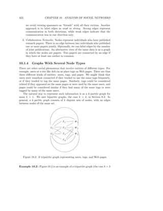
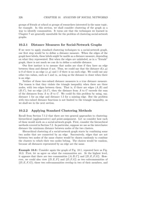

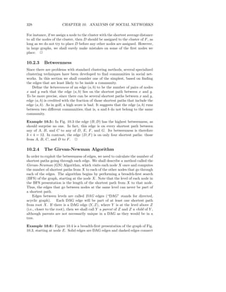
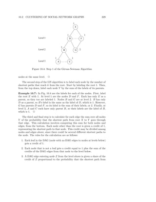
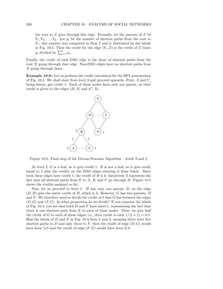
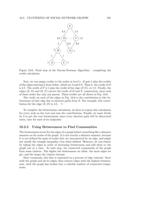
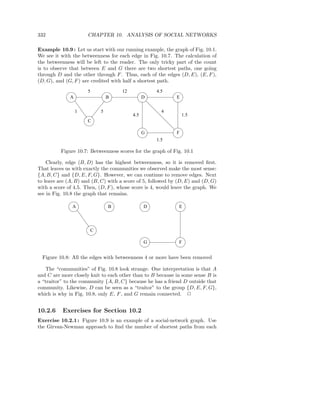
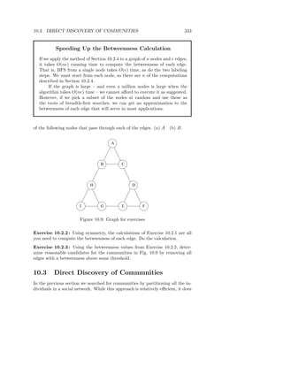
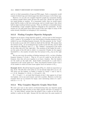
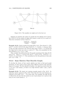
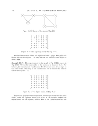
![10.4. PARTITIONING OF GRAPHS 341
the same entries as D on the diagonal. Off the diagonal, at row i and column j,
L has −1 if there is an edge between nodes i and j and 0 if not.
Example 10.18 : The Laplacian matrix for the graph of Fig. 10.12 is shown
in Fig. 10.15. Notice that each row and each column sums to zero, as must be
the case for any Laplacian matrix. 2
2 -1 -1 0 0 0 0
-1 3 -1 -1 0 0 0
-1 -1 2 0 0 0 0
0 -1 0 4 -1 -1 -1
0 0 0 -1 2 -1 0
0 0 0 -1 -1 3 -1
0 0 0 -1 0 -1 2
Figure 10.15: The Laplacian matrix for Fig. 10.12
10.4.4 Eigenvalues of the Laplacian Matrix
We can get a good idea of the best way to partition a graph from the eigenvalues
and eigenvectors of its Laplacian matrix. In Section 5.1.2 we observed how
the largest eigenvalue of the transition matrix of the Web told us something
useful about the importance of Web pages. In fact, in simple cases (no taxation)
the eigenvector associated with the largest eigenvalue is the PageRank vector.
When dealing with the Laplacian matrix, however, it turns out that the smallest
eigenvalues and their eigenvectors reveal the information we desire.
The smallest eigenvalue for every Laplacian matrix is 0. and its correspond-
ing eigenvector is [1, 1, . . . , 1]. To see why, let L be the Laplacian matrix for a
graph of n nodes, and let 1 be the column vector of all 1’s with length n. We
claim L1 is a column vector of all 0’s. To see why, consider row i of L. Its
diagonal element has the degree d of node i. Row i also will have d occurrences
of −1, and all other elements of row i are 0. Multiplying row i by 1 has the
effect of summing the row, and this sum is clearly d + (−1)d = 0. Thus, we
can conclude L1 = 01, which demonstrates that 0 is an eigenvalue and 1 its
corresponding eigenvector.
While we shall not prove this fact, there is a simple way to find the second-
smallest eigenvalue for any matrix, such as the Laplacian matrix, that is sym-
metric (the entry in row i and column j equals the entry in row j and column
i). Then the second-smallest eigenvector of L is the minimum of xT Lx, where
x = [x1 , x2 , . . . , xn ] is a column vector with n components, and the minimum
is taken under the constraints:
n
1. The length of x is 1; that is i=1 x2 = 1.
i](https://image.slidesharecdn.com/miningofmassivedatasets-120805173332-phpapp01/85/Mining-of-massive-datasets-357-320.jpg)
![342 CHAPTER 10. ANALYSIS OF SOCIAL NETWORKS
n
2. x is orthogonal to the smallest eigenvector 1; that is, xT 1 = i=1 xi = 0.
Moreover, the value of x that achieves this minimum is the second eigenvector.
When L is a Laplacian matrix for an n-node graph, the expression xT Lx
has a useful equivalent expression. Recall that L = D − A, where D and
A are the degree and adjacency matrices of the same graph. Thus, xT Lx =
xT Dx − xT Ax. Let us evaluate the term with D and then the term for A. Dx
is the column vector [d1 x1 , d2 x2 , . . . , dn xn ], where di is the degree of the ith
node of the graph. Thus, xT Dx is n di x2 . i=1 i
Now, turn to xT Ax. The ith component of the column vector Ax is the
sum of −xj over all j such that there is an edge (i, j) in the graph. Thus,
xT Ax is the sum of −2xi xj over all pairs of nodes {i, j} such that there is
an edge between them. Note that the factor 2 appears because each set {i, j}
corresponds to two terms, −xi xj and −xj xi .
We can group the terms of xT Lx in a way that distributes the terms to
each pair {i, j}. From A, we already have the term −2xi xj . From D, we
distribute the term di x2 to the di pairs that include node i. As a result, we
i
can associate with each pair {i, j} that has an edge between nodes i and j the
terms x2 − 2xi xj + x2 . This expression is equivalent to (xi − xj )2 . Therefore, we
i j
have proved that xT Lx equals the sum over all graph edges (i, j) of (xi − xj )2 .
Recall that the second-smallest eigenvalue is the minimum of this expression
n
under the constraint that i=1 x2 = 1. Intuitively, we minimize it by making
i
xi and xj close whenever there is an edge between nodes i and j in the graph.
√
We might imagine that we could choose xi = 1/ n for all i and thus make this
sum 0. However, recall that we are constrained to choose x to be orthogonal to
1, which means the sum of the xi ’s is 0. We are also forced to make the length
of x be 1, so all components cannot be 0. As a consequence, x must have some
positive and some negative components.
We can obtain a partition of the graph by taking one set to be the nodes
i whose corresponding vector component xi is positive and the other set to
be those whose components are negative. This choice does not guarantee a
partition into sets of equal size, but the sizes are likely to be close. We believe
that the cut between the two sets will have a small number of edges because
(xi −xj )2 is likely to be smaller if both xi and xj have the same sign than if they
have different signs. Thus, minimizing xT Lx under the required constraints will
tend to give xi and xj the same sign if there is an edge (i, j).
1 4
2 5
3 6
Figure 10.16: Graph for illustrating partitioning by spectral analysis](https://image.slidesharecdn.com/miningofmassivedatasets-120805173332-phpapp01/85/Mining-of-massive-datasets-358-320.jpg)
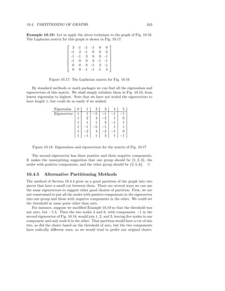
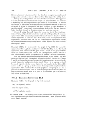
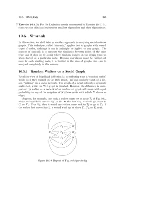
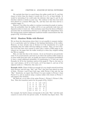
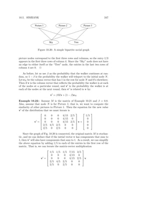
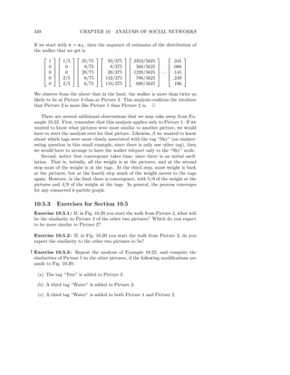
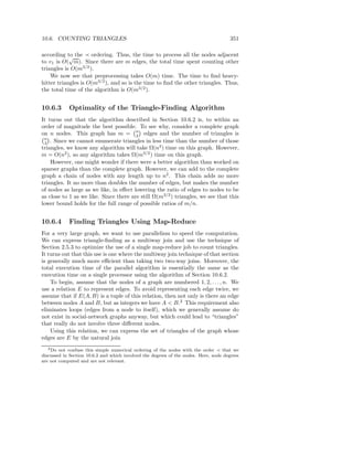
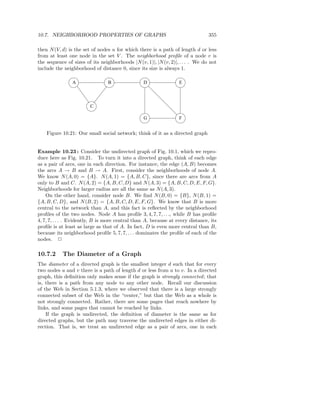
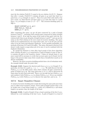
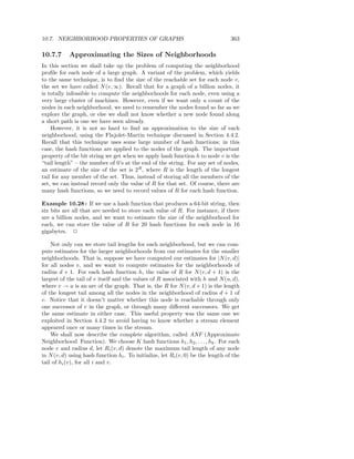
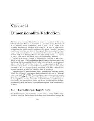
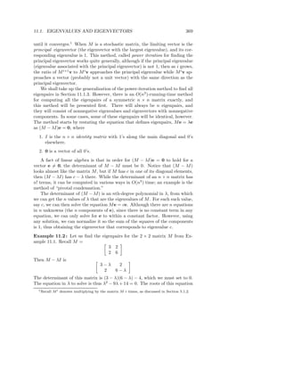
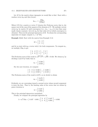
![11.1. EIGENVALUES AND EIGENVECTORS 373
Example 11.5 : For the matrix M of Example 11.2, the matrix E is
√ √
2/√5 1/√5
−1/ 5 2/ 5
E T is therefore √ √
2/√5 −1/√5
1/ 5 2/ 5
When we compute EE T we get
4/5 + 1/5 −2/5 + 2/5 1 0
=
−2/5 + 2/5 1/5 + 4/5 0 1
The calculation is similar when we compute E T E. Notice that the 1’s along
the main diagonal are the sums of the squares of the components of each of the
eigenvectors. which makes sense because they are unit vectors. The 0’s off the
diagonal reflect the fact that the entry in the ith row and jth column is the
dot product of the ith and jth eigenvectors. Since eigenvectors are orthogonal,
these dot products are 0. 2
11.1.5 Exercises for Section 11.1
Exercise 11.1.1 : Find the unit vector in the same direction as the vector
[1, 2, 3].
Exercise 11.1.2 : For any symmetric 3 × 3 matrix
a−λ b c
b d−λ e
c e f −λ
there is a cubic equation in λ that says the determinant of this matrix is 0. In
terms of a through f , find this equation.
Exercise 11.1.3 : Find the eigenpairs for the following matrix:
1 1 1
1 2 3
1 3 5
using the method of Section 11.1.2.
! Exercise 11.1.4 : Find the eigenpairs for the following matrix:
1 1 1
1 2 3
1 3 6
using the method of Section 11.1.2.](https://image.slidesharecdn.com/miningofmassivedatasets-120805173332-phpapp01/85/Mining-of-massive-datasets-389-320.jpg)
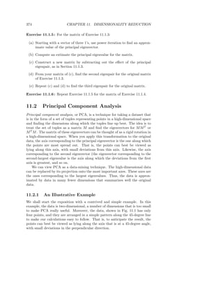
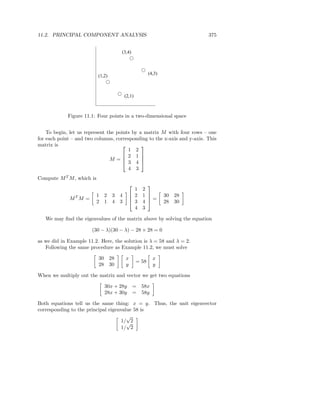
![376 CHAPTER 11. DIMENSIONALITY REDUCTION
For the second eigenvalue, 2, we perform the same process. Multiply out
30 28 x x
=2
28 30 y y
to get the two equations
30x + 28y = 2x
28x + 30y = 2y
Both equations tell us the same thing: x = −y. Thus, the unit eigenvector
corresponding to the principal eigenvalue 2 is
√
−1/√2
1/ 2
While we promised to write eigenvectors with their first component positive,
we choose the opposite here because it makes the transformation of coordinates
easier to follow in this case.
Now, let us construct E, the matrix of eigenvectors for the matrix M T M .
Placing the principal eigenvector first, the matrix of eigenvectors is
√ √
1√2 −1√2
E=
1 2 1 2
Any matrix of orthonormal vectors (unit vectors that are orthogonal to one
another) represents a rotation of the axes of a Euclidean space. The matrix
above can be viewed as a rotation 45 degrees counterclockwise. For example,
let us multiply the matrix M that represents each of the points of Fig. 11.1 by
E. The product is
√ √
1 2 √ √ 3/√2 1/√2
2 1 1 2 −1 2 3/ 2 −1/ 2
ME = √ √ = √ √
3 4 1 2 1 2 7/ 2 1/√2
√
4 3 7/ 2 −1/ 2
For example, the first point, [1, 2], has been transformed into the point
√ √
[3 2, 1/ 2]
If we examine Fig. 11.2, with the dashed line representing the new x-axis, we √
see
that the projection of the first point onto that axis places it at distance 3/ 2
from the origin. To check that fact, notice that the point of projection for both
the first and second points is [1.5, 1.5] in the original coordinate system, and
the distance from the origin of this point is
√
(1.5)2 + (1.5)2 = 9/2 = 3/ 2](https://image.slidesharecdn.com/miningofmassivedatasets-120805173332-phpapp01/85/Mining-of-massive-datasets-392-320.jpg)
![11.2. PRINCIPAL COMPONENT ANALYSIS 377
(3,4)
(3.5,3.5)
(4,3)
(1,2)
(1.5,1.5)
(2,1)
Figure 11.2: Figure 11.1 with the axes rotated 45 degrees counterclockwise
Moreover, the new y-axis is,√ course, perpendicular to the dashed line. The
of
first point is at distance 1/ 2 above the new x-axis in the direction of the
y-axis. That is, the distance between the points [1, 2] and [1.5, 1.5] is
√
(1 − 1.5)2 + (2 − 1.5)2 = (−1/2)2 + (1/2)2 = 1/2 = 1/ 2
Figure 11.3 shows the four points in the rotated coordinate system.
(3/ 2 , 1/ 2 ) (7/ 2 , 1/ 2 )
(3/ 2 , −1/ 2 ) (7/ 2 , −1/ 2 )
Figure 11.3: The points of Fig. 11.1 in the new coordinate system
The second point, [2, 1] happens by coincidence to project onto the same
√
point of the new x-axis. It is 1/ 2 below that axis along the new y-axis, as is
confirmed by √ fact that the second row in the matrix of transformed points
√ the √ √
is [3/ 2, −1/ 2]. The third point, [3, 4] is transformed into [7/ 2, 1/ 2] and
√ √
the fourth point, [4, 3], is transformed to [7/ 2, −1/ 2]. That is, they both
√
project onto the same point of the √ x-axis, and that point is distance 7/ 2
new
from the origin, while they are 1/ 2 above and below the new x-axis in the
direction of the new y-axis.
11.2.2 Using Eigenvectors for Dimensionality Reduction
From the example we have just worked, we can see a general principle. If M is a
matrix whose rows each represent a point in a Euclidean space with any number](https://image.slidesharecdn.com/miningofmassivedatasets-120805173332-phpapp01/85/Mining-of-massive-datasets-393-320.jpg)
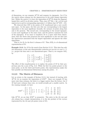
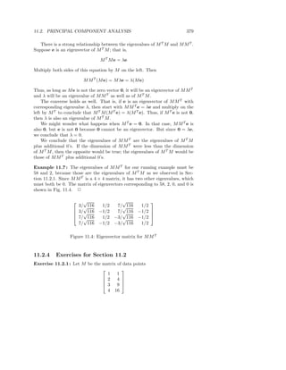

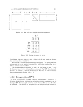
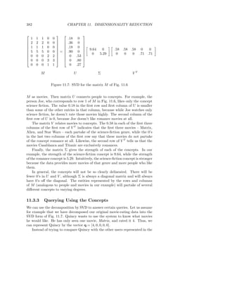
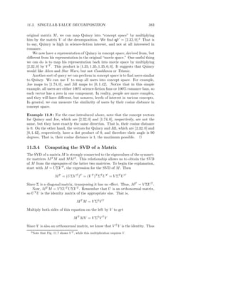
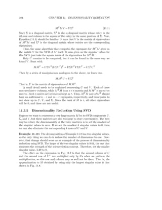
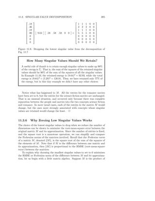
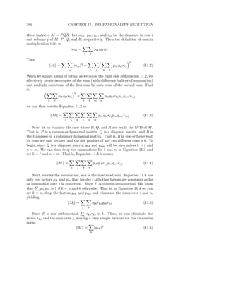
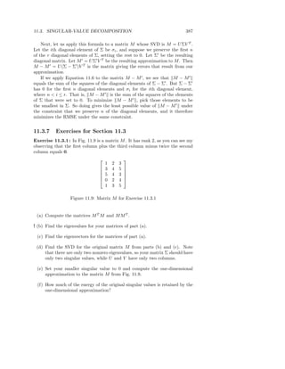
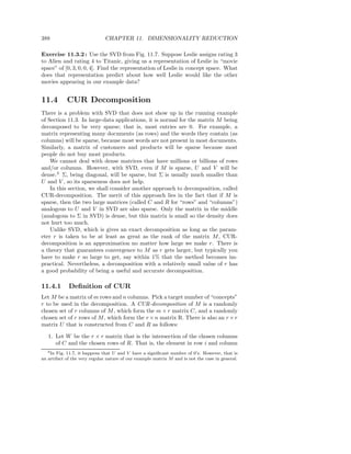
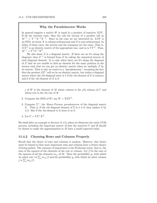
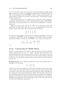
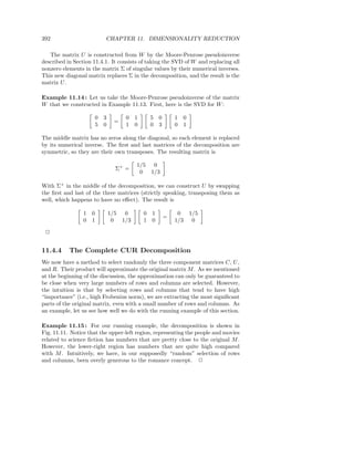
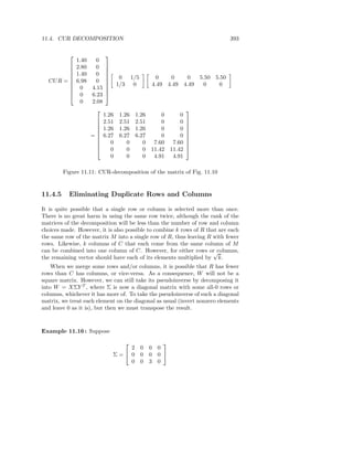
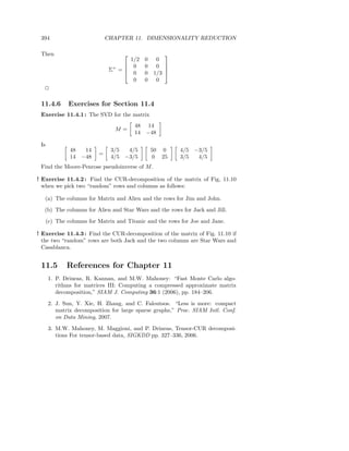
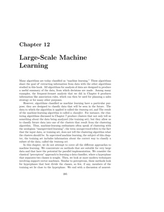
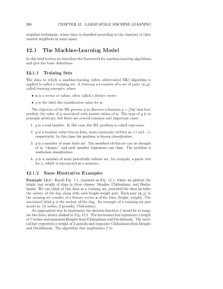
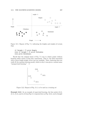
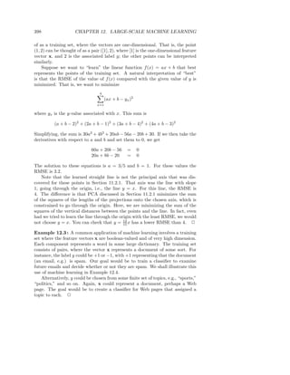
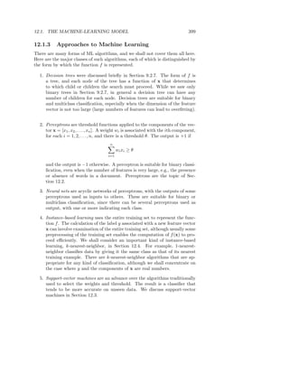
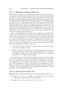
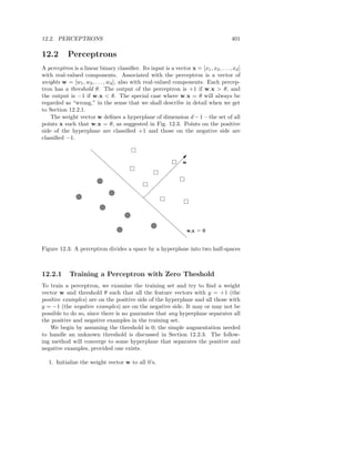
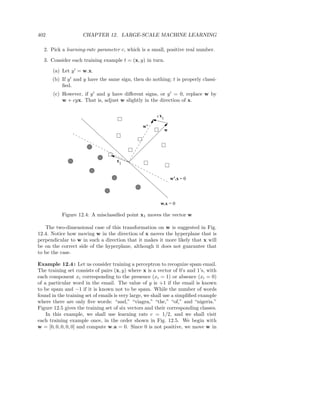
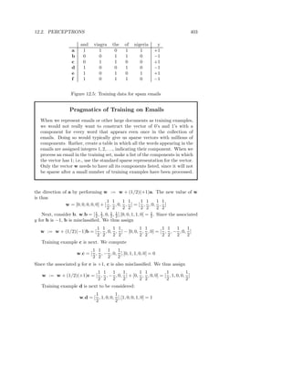
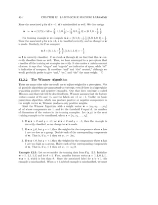
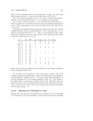
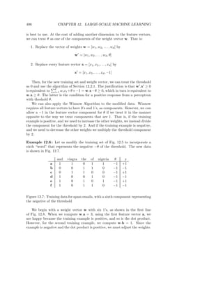
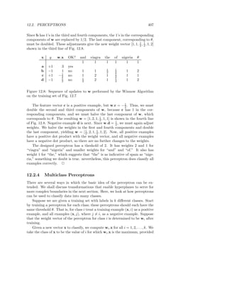

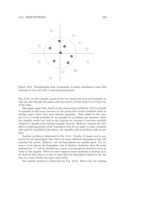
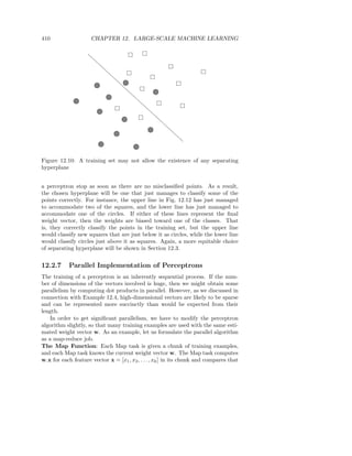
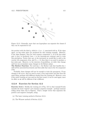
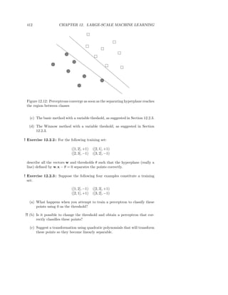
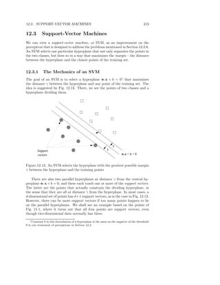
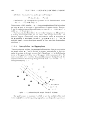
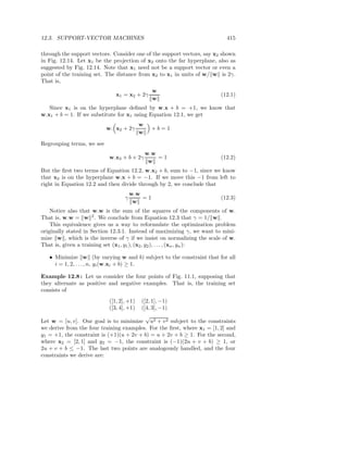
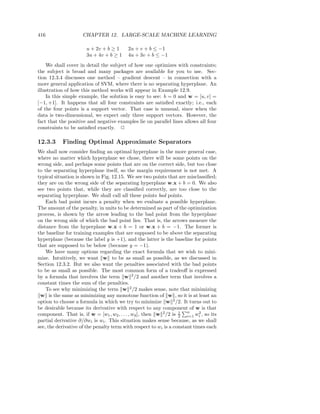
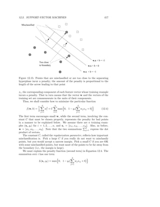
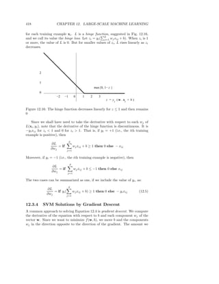
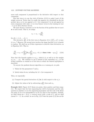
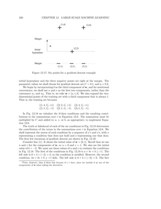
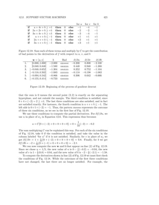
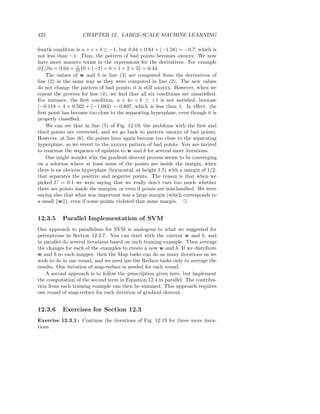
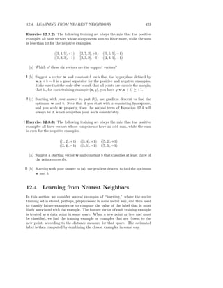
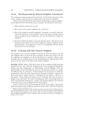
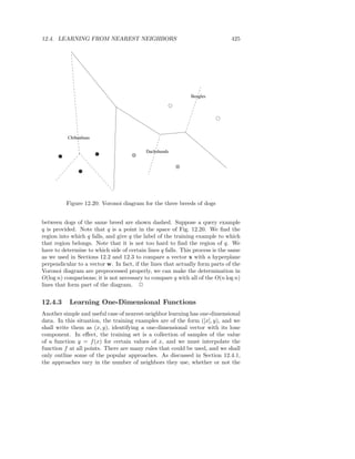
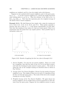
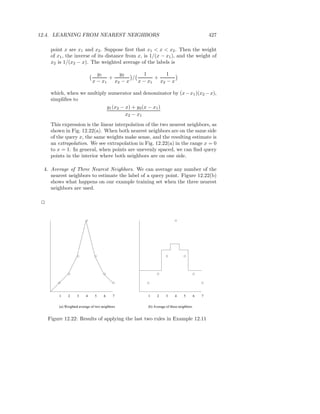
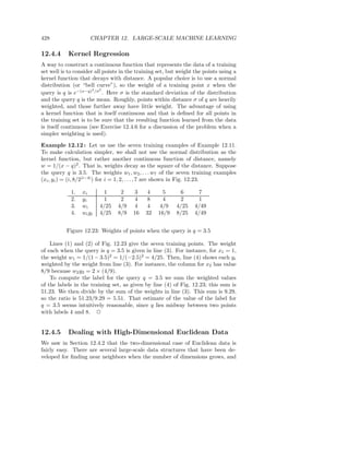
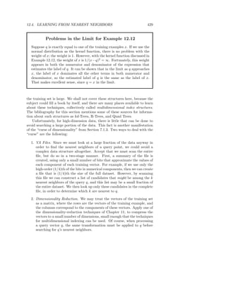


This document is the preface to the book "Mining of Massive Datasets" by Anand Rajaraman and Jeffrey D. Ullman. It provides an overview of the book, which covers topics related to applying algorithms to very large datasets, including distributed file systems, map-reduce, similarity search, data streams, search engines, frequent patterns, clustering, and applications like advertising and recommendations. The preface outlines the book's content, prerequisites, and acknowledges contributions from others.


![[Estácio - IESAM] Automatizando Tarefas com Gulp.js](https://cdn.slidesharecdn.com/ss_thumbnails/estcio-iesamautomatizandotarefascomgulp-151220144313-thumbnail.jpg?width=640&height=640&fit=bounds)


![Getting Started with Apache Spark: Big Data Made Simple [Free Meetup]](https://cdn.slidesharecdn.com/ss_thumbnails/apachesparkgettingstarted-260203175547-8361bcc3-thumbnail.jpg?width=640&height=640&fit=bounds)


