The document is a user manual for the Eclipse system, detailing its installation, operation, and programming features. It covers various aspects, including troubleshooting, terminology, development tools, compiler specifics, and module systems. The manual serves as a comprehensive guide for users seeking to understand and utilize Eclipse effectively.


![Chapter 1
Introduction
1.1 What is ECLi
PSe
?
ECLiPSe (ECLiPSe Constraint Logic Programming System) is an open-source software system
whose aim is to serve as a platform for integrating various Logic Programming extensions. It is
used in particular for the cost-effective development and deployment of constraint programming
applications, e.g. in the areas of planning, scheduling, resource allocation, timetabling, transport
etc. It is also ideal for teaching most aspects of combinatorial problem solving, e.g. problem
modelling, constraint programming, mathematical programming, and search techniques. It con-
tains several constraint solver libraries, a high-level modelling and control language, interfaces
to third-party solvers, an integrated development environment and interfaces for embedding into
host environments.
The ECLiPSe programming language has been developed from the Prolog language ([3]), more
specifically the Edinburgh family of Prologs and more recently the ISO Prolog standard ([1]).
ECLiPSe retains backward compatibility by supporting several language dialects.
In terms of implementation technology, ECLiPSe is built around an incremental compiler which
compiles ECLiPSe source into WAM-like code [14], and a runtime system comprising an emulator
of this abstract code, automatic memory management, I/O system and built-in predicates.
1.2 Overview
The ECLiPSe logic programming system was originally an integration of ECRC’s SEPIA, Mega-
Log and (parts of the) CHIP systems. It was then further developed into a Constraint Logic
Programming system with a focus on hybrid problem solving and solver integration. The docu-
mentation is organised as follows:
The User Manual describes the functionality of the ECLiPSe kernel (this document).
The Constraint Library Manual describes the major ECLiPSe libraries, in particular the ones
implementing constraint solvers.
The Interfacing and Embedding Manual describes how to interface ECLiPSe to other program-
ming languages, and in particular how to embed it into an application as a component.
The Reference Manual contains detailed descriptions of all the Built-in predicates and the li-
braries. This information is also available from the development system’s help/1 command
1](https://image.slidesharecdn.com/userman-230228072618-efbbcc3a/85/eclipse-pdf-13-320.jpg)


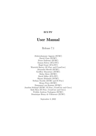
![where Head is a head.
A fact may be considered to be a rule whose body is always true.
Functor A functor is characterised by its name (which is an atom), and its arity (which is its
number of arguments).
Goal Clause See query.
Ground A term is ground when it does not contain any uninstantiated variables.
Head A clause head is a structure or an atom.
Instantiated A variable is instantiated when it has been bound to an atomic or a compound
term as opposed to being uninstantiated or free. See also ground.
List A list is a special type of term within Prolog. It is a recursive data structure consisting of
pairs (whose tails are lists). A list is either the atom [] called nil as in LISP, or a pair
whose tail is a list. The notation :
[a , b , c]
is shorthand for:
[a | [b | [c | []]]]
Mode A predicate mode is a particular instantiation pattern of its arguments at call time. Such
a pattern is usually written as a predicate template, e.g.,
p(+,-)
where the symbols +, ++, - and ? represent instantiated, ground, uninstantiated and
unknown arguments respectively.
Name/Arity The notation Name/Arity is used to specify a functor by giving its name and arity.
Number A number literal denotes a number, more or less like in all programming languages.
Pair A pair is a compound term with the functor ./2 (dot) which is written as :
[H|T]
H is the head of the pair and T its tail.
Predicate A predicate is another term for a procedure.
PredSpec This is similar to Name/Arity. Some built-ins allow the arity to be omitted and to
specify the name only: this stands for all (visible) predicates with that name and any arity.
Program Clause A program clause (or simply clause) is either the term
Head :- Body.
(i.e., a compound term with the functor :-/2), or only a fact.
5](https://image.slidesharecdn.com/userman-230228072618-efbbcc3a/85/eclipse-pdf-17-320.jpg)


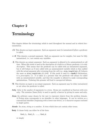
![3.5 How do I use eclipse?
3.5.1 Getting started
To start ECLiPSe, type the command eclipse at an operating system command-line prompt.
This will display something like this:
% eclipse
ECLiPSe Constraint Logic Programming System [kernel]
Kernel and basic libraries copyright Cisco Systems, Inc.
and subject to the Cisco-style Mozilla Public Licence 1.1
(see legal/cmpl.txt or eclipseclp.org/licence)
Source available at www.sourceforge.org/projects/eclipse-clp
GMP library copyright Free Software Foundation, see legal/lgpl.txt
For other libraries see their individual copyright notices
Version X.Y #Z, DAY MONTH DD HH:MM YYYY
[eclipse 1]:
The list in square brackets on the first line specifies the configuration of the running system,
i.e., the language extensions that are present. The copyright and version information is followed
by the prompt [eclipse 1]:, which tells the user that the top-level loop is waiting for a user
query in the module eclipse. The predicate help/0 gives general help and help/1 gives help
about specific built-in predicates.
3.5.2 Interacting with the top level loop
The ECLiPSe prompt [eclipse 1]: indicates that ECLiPSe is at the top level and the opened
module is eclipse. The top level loop is a procedure which repetitively prompts the user for a
query, executes it and reports its result, i.e., either the answer variable bindings or the failure
message. There is always exactly one module opened in the top level and its name is printed in
the prompt. From this point it is possible to enter ECLiPSe goals, e.g., to pose queries, to enter
an ECLiPSe program from the keyboard or to compile a program from a file. Goals are entered
after the prompt and are terminated by fullstop and newline.
The ECLiPSe system may be exited by typing CTRL-D (UNIX) or CTRL-Z + RETURN (Windows)
at the top level prompt, or by calling either the halt/0 or the exit/1 predicates.
3.5.3 Compiling a program
The square brackets [...] or the compile/1 predicate are used to compile ECLiPSe source from
a file. If the goal
compile(myfile).
or the short-hand notation
[myfile].
is called, either as a query at the top level or within another goal, the system looks for the file
myfile or for a file called myfile.pl or myfile.ecl and compiles it. The short-hand notation
may also be used to compile several files in sequence:
12](https://image.slidesharecdn.com/userman-230228072618-efbbcc3a/85/eclipse-pdf-24-320.jpg)
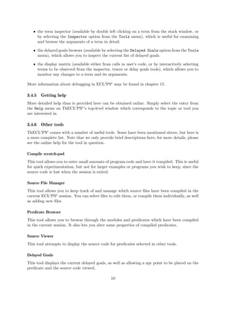
![[ file_1, file_2, ..., file_n ]
The compile/2 predicate may be used to compile a file or list of files into a module specified in
the second argument.
If a file has been modified since it was compiled, it may be recompiled by invoking the make/0
predicate. This recompiles any files which have become out-of-date.
For more information on program compilation and the compiler, please see chapter 6.
3.5.4 Entering a program from the terminal
Programs can be entered directly from the terminal, as well as being read from files. To do
this, simply compile the special file user. That is, [user]. or compile(user). at a top
level prompt. The system then displays the compiler prompt (which is a blank by default) and
waits for a sequence of clauses. Each of the clauses is terminated by a fullstop. (If the fullstop
is omitted the system just sits waiting, because it supposes the clause is not terminated. If
you omit the fullstop by accident simply type it in on the following line, and then proceed to
type in the program clauses, each followed by a fullstop and carriage return.) To return to the
top level prompt, type CTRL-D (UNIX), CTRL-Z + RETURN (Windows) or enter the atom
end_of_file followed by fullstop and RETURN.
For example:
[eclipse 1]: [user].
source_processor.eco loaded in 0.01 seconds
...
ecl_compiler.eco loaded in 0.23 seconds
father(abraham, isaac).
father(isaac, jacob).
father(jacob, joseph).
ancestor(X, Y) :- father(X, Y).
ancestor(X, Y) :- ancestor(X, Z), ancestor(Z, Y).
^D
tty compiled 420 bytes in 0.01 seconds
Yes (0.24s cpu)
[eclipse 2]:
The two predicates father/2 and ancestor/2 are now compiled and can be used.
3.5.5 Executing a query
Once a set of clauses has been compiled, it may be queried in the usual Prolog manner. If
there are uninstantiated variables in the query, the system will attempt to find an instantiation
of them which will satisfy the query, and if successful it will display one such instantiation. If
potentially there is another solution, the top level will then wait for a further instruction: either
a <CR> (“newline” or “return”) or a semi-colon (;). A return will end the query successfully.
A semi-colon will initiate backtracking in an attempt to find another solution to the query.
Note that it is not necessary to type a new line after the semicolon — one keystroke is enough.
When the top level loop can detect that there are no further solutions, it does not wait for the
13](https://image.slidesharecdn.com/userman-230228072618-efbbcc3a/85/eclipse-pdf-25-320.jpg)
![semicolon or newline, but it displays directly the next prompt. For example in a query on a
family database:
[eclipse 3]: father(X, Y).
X = abraham
Y = isaac
Yes (0.00s cpu, solution 1, maybe more) ? ; (user types ’;’)
X = isaac
Y = jacob
Yes (0.00s cpu, solution 2)
[eclipse 4]:
Queries may be extended over more than one line. When this is done the prompt changes to a
tabulation character, i.e., the input is indented to indicate that the query is not yet completed.
The fullstop marks the end of the input.
3.5.6 Interrupting the execution
If a program is executing, it may be interrupted by typing CTRL-C (interrupt in the UNIX
environment). This will invoke the corresponding interrupt handler (see section 14.3). By
default, the system prints a menu offering some alternatives:
^C
interruption: type a, b, c, e, or h for help : ? h (user types ’h’)
help
a : abort
b : break level
c : continue
e : exit
h : help
interruption: type a, b, c, e, or h for help : ?
The a option returns to the toplevel, b starts a nested toplevel, c continues the interrupted
execution, and e is an emergency exit of the whole ECLiPSe session. If the debugger is running,
an additional option d is displayed: it switches the debugger to creep mode.
The execution of ECLiPSe may be suspended by typing CTRL-Z (suspend) or by calling pause/0.
This will suspend the ECLiPSe process and return the UNIX prompt. Entering the shell com-
mand fg will return to ECLiPSe. Note that this feature may not be available on all systems.
3.5.7 Debugging a program
Please see the chapters on debugging in the tutorial and user manuals for more details. The
tutorial chapter covers the TkECLiPSe debugging in a tutorial style tour, and the user manual
chapter covers debugging in general and the command-line debugger in particular.
14](https://image.slidesharecdn.com/userman-230228072618-efbbcc3a/85/eclipse-pdf-26-320.jpg)
![3.5.8 The history mechanism
The ECLiPSe toplevel loop provides a simple history mechanism which allows the examination
and repetition of previous queries. The history list is printed with the command h. A previous
query is invoked by typing either its absolute number or its relative negative offset from the
current query number (i.e., –1 will execute the previous query). The current query number is
displayed in the toplevel prompt.
The history is initialized from the file .eclipse_history in the current directory or in the home
directory. This file contains the history goals, each ended by a fullstop. The current history can
be written using the predicate write history/0 from the util library.
3.5.9 Getting help
Detailed documentation about all the predicates in the ECLiPSe libraries can be obtained online
through the help facility. It has two modes of operation. First, when a fragment of a built-in
name is specified, a list of short descriptions of all built-ins whose name contains the specified
string is printed. For example,
:- help(write).
will print one-line descriptions about write/1, writeclause/2, etc. When a unique specification
is given, the full description of the specified built-in is displayed, e.g., in
:- help(write/1).
3.6 How do I make things happen at compile time?
A file being compiled may contain queries. These are goals preceded by the symbol “:-”. As soon
as a query is encountered in the compilation of a file, the ECLiPSe system will try to satisfy it.
Thus by inserting goals in this fashion, things can be made to happen at compile time.
In particular, a file can contain a directive to the system to compile another file, and so large
programs can be split between files, while still only requiring a single simple command to compile
them. When this happens, ECLiPSe interprets the pathnames of the nested compiled files
relative to the directory of the parent compiled file; if, for example, the user calls
[eclipse 1]: compile(’src/pl/prog’).
and the file src/pl/prog.pl contains a query
:- [part1, part2].
then the system searches for the files part1.pl and part2.pl in the directory src/pl and not in
the current directory. Usually larger ECLiPSe programs have one main file which contains only
commands to compile all the subfiles. In ECLiPSe it is possible to compile this main file from
any directory. (Note that if your program is large enough to warrant breaking into multiple files
(let alone multiple directories), it is probably worth turning the constituent components into
modules — see chapter 8.)
15](https://image.slidesharecdn.com/userman-230228072618-efbbcc3a/85/eclipse-pdf-27-320.jpg)
![3.7 How do I use ECLi
PSe
libraries in my programs?
A number of files containing library predicates are supplied with the ECLiPSe system. These
predicates provide utility functions for general use. They are usually installed in an ECLiPSe
library directory (or directories). These predicates are either loaded automatically by ECLiPSe
or may be loaded “by hand”.
During the execution of an ECLiPSe program, the system may dynamically load files containing
library predicates. When this happens, the user is informed by a compilation or loading mes-
sage. It is possible to explicitly force this loading to occur by use of the lib/1 or use module/1
predicates. e.g., to load the library called lists, use one of the following goals:
lib(lists)
use_module(library(lists))
This will load the library file unless it has been already loaded. In particular, a program can
ensure that a given library is loaded when it is compiled, by including an appropriate directive
in the source, e.g., :- lib(lists).
Library files are found by searching the library path and by appending a suffix to the library
name. The search path used when loading libraries is specified by the global flag library_path
using the get flag/2 and set flag/2 predicates. This flag contains a list of strings containing the
pathnames of the directories to be searched when loading a library file. User libraries may be
be added to the system simply by copying the desired file into the ECLiPSe library directory.
Alternatively the library_path flag may be updated to point at a number of user specific
directories. The following example illustrates how a directive may be added to a file to add a
user-defined library in front of any existing system libraries.
?- get_flag(library_path,Path),
set_flag(library_path, ["/home/myuser/mylibs" | Path]).
The UNIX environment variable ECLIPSELIBRARYPATH may also be used to specify the initial
setting of the library path. The syntax is similar to the syntax of the UNIX PATH variable, i.e.,
a list of directory names separated by colons. The directories will be prepended to the standard
library path in the given order.
3.8 How do I make my programs run faster?
By default, ECLiPSe compiles programs as traceable, which means that they can be traced
using the built-in debugger. To obtain maximum efficiency, the directive nodbgcomp/0 should
be used, which will set some flags to produce a more efficient and shorter code:
[eclipse 2]: nodbgcomp.
yes.
[eclipse 3]: [user].
father(abraham, isaac).
father(isaac, jacob).
father(jacob, joseph).
ancestor(X, Y) :- father(X, Y).
ancestor(X, Y) :- ancestor(X, Z), ancestor(Z, Y).
16](https://image.slidesharecdn.com/userman-230228072618-efbbcc3a/85/eclipse-pdf-28-320.jpg)
![user compiled optimized 396 bytes in 0.02 seconds
yes.
[eclipse 4]:
Section 6.7 contains more detailed discussion on other techniques which can be used to optimise
your programs.
3.9 Other tips
3.9.1 Initialization at start-up
If you wish to have ECLiPSe do or execute things at startup time, you can achieve this in
TkECLiPSe by setting the initial query call in the Preference editor; and in the command-line
eclipse by putting via a .eclipserc file.
For eclipse, before displaying the initial prompt, the system checks whether there is a file
called .eclipserc in the current directory and if not, in the user’s home directory. If such a file
is found, ECLiPSe compiles it first. Thus it is possible to put various initialization commands
into this file. ECLiPSe has many possibilities to change its default behaviour and setting up a
.eclipserc file is a convenient way to achieve this. A different name for the initialization file
can be specified in the environment variable ECLIPSEINIT. If ECLIPSEINIT is set to an empty
string, no initialization is done. If the system is started with a -e option, then the .eclipserc
file is ignored.
For TkECLiPSe, the system will make the initial query call as set in the Preference Editor before
giving control to the user. This call can be set to compile an initialization file. This can be
the .eclipserc file, or some other file if the user wants to initialize the system differently in
TkECLiPSe.
3.9.2 Recommended file names
It is recommended programming practice to give the Prolog source programs the suffix .pl, or
.ecl if it contains ECLiPSe specific code. It is not enforced by the system, but it simplifies
managing the source programs. The compile/1 predicate automatically adds the suffix to the
file name, so that it does not have to be specified; if the literal file name can not be found,
the system tries appending each of the valid suffixes in turn and tries to find the resulting file
name. The system’s list of valid Prolog suffixes is in the global flag prolog_suffix and can
be examined and modified using get flag/2 and set flag/2. For example, to add the new suffix
.pro use:
get_flag(prolog_suffix, Old), set_flag(prolog_suffix, [".pro"|Old]).
17](https://image.slidesharecdn.com/userman-230228072618-efbbcc3a/85/eclipse-pdf-29-320.jpg)

![Chapter 4
The TkECLiPSe Development Tools
TkECLiPSe is a graphical user interface to ECLiPSe. It is an alternative to the traditional
textual line-based user interface, providing multiple windows, menus and buttons to assist the
user in interacting with ECLiPSe. It consists of two major components:
ˆ A graphical top-level.
ˆ A suite of development tools for aiding the development of ECLiPSe code.
TkECLiPSe is implemented in the Tcl/Tk scripting language/graphical toolkit [12], using the
new ECLiPSe Tcl/Tk interface [11]. The development tools are designed to be independent of
the top-level, so the users can develop their own applications with a graphical front end written
in Tcl/Tk, replacing the TkECLiPSe top-level, but still using the development tools.
Chapter 3 gave an introduction to using TkECLiPSe from a user’s point of view. This chapter
focuses on how to use the tools from a programmer’s point of view (i.e., how to include them in
a program). In particular it discusses in detail the display matrix tool, which can be invoked in
user’s ECLiPSe code; and also how to use the development tools in the user’s own applications.
4.1 Display Matrix
This tool provides a method to display the values of terms in a matrix form. It is particularly
useful because it can display the attributes of an attributed variable.1 The predicate which
invokes the display matrix is considered a no-op in the tty-based ECLiPSe,2 and so the same
code can be run without modification from either eclipse or tkeclipse, though the matrix
display is only presented to the user in the latter.
To invoke this tool use either make display matrix/2 or make display matrix/5. Adding a call
to one of these predicates should be the only change you need to make to your code. For example,
in the following fragment of a N-queens program, only one extra line has been added to invoke
a display matrix:
1
The display matrix tool is similar to the variable display of Grace. The main differences are: it can display
all attributes, not just the finite domain attribute; the attributes can only be observed, not changed; and the
labelling strategy cannot be changed.
2
Unless it is attached to the remote development tools, in which case the display matrix is invoked.
19](https://image.slidesharecdn.com/userman-230228072618-efbbcc3a/85/eclipse-pdf-31-320.jpg)


![Figure 4.3: Remote Development Tools Toplevel (left: ECLiPSe active; right: remote tools
active)
flow of control between them: only one process can be ‘active’ at any time. The interaction
is similar to the standard interaction between a debugger and the program being debugged
– debugging commands can only be issued while the execution of the program is suspended.
In the same way, the user can only interact with the remote tools window when execution in
the ECLiPSe session is suspended. The toplevel window of the remote tools has an indicator
showing which side has control (see Figure 4.3). To allow ECLiPSe to resume execution, control
is transferred back from the remote tools to ECLiPSe. This can either be done automatically
from the tools (e.g., when one of the debug buttons is pressed in the tracer tool), or control
can be transferred explicitly back to ECLiPSe via the “Resume ECLiPSe” button on the remote
tools window.
Starting Remote Tools
To use the remote tools, the user must first load the right library with lib(remote_tools).
After loading the library, the user can start the remote tools by starting the development tools
as a separate program and then manually attaching the program to the ECLiPSe session. This
allows the development tools to be run on a different machine from the ECLiPSe session. In
this case, the user initiates the attachment in ECLiPSe with attach tools/0:
[eclipse 2]: attach_tools.
Socket created at address holborn.icparc.ic.ac.uk/22849
ECLiPSe prints the host and port address it expects the remote tools to attach to, and execution
is now suspended waiting for the remote tools to attach. This is done by running the tktools
program, which is located with the other ECLiPSe executables. As stated, this program can be
run on a different machine from the ECLiPSe session, as long as the two are connected via a
network such as the internet. A connection window is then displayed as shown:
23](https://image.slidesharecdn.com/userman-230228072618-efbbcc3a/85/eclipse-pdf-35-320.jpg)


![5.1.1 Updating Structures
To construct an updated structure, i.e., a structure which is similar to an existing structure
except that one or more fields have new values, use the update struct/4 built-in, which allows
you to do that without having to mention all the other field names in the structure.
5.1.2 Arity and Functor of Structures
The arity of a structure can be symbolically written using of/2 as follows:
property(arity) of StructName
For example,
?- printf("A book has %d fields%n", [property(arity) of book]).
A book has 4 fields
Yes.
Similarly, the whole StructName/Arity specification can be written as
property(functor) of StructName
which is used for the portray-declaration in the example below.
5.1.3 Printing Structures
When structures are printed, they are not translated back into the abstract structure syntax by
default. The reason this is not done is that this can be bulky if all fields are printed, and often
it is desirable to hide some of the fields anyway.
A good way to control printing of big structures is to write customized portray-transformations
for them, for instance
:- local portray(property(functor) of book, tr_book_out/2, []).
tr_book_out(book{author:A,title:T},
no_macro_expansion(book{author:A,title:T})).
which will cause book/4 structures to be printed like
book{author:twain, title:tom sawyer}
while the other two arguments remain hidden.
5.1.4 Inheritance
Structures can be declared to contain other structures, in which case they inherit the base
structure’s field names. Consider the following declarations:
:- local struct(person(name,address,age)).
:- local struct(employee(p:person,salary)).
The employee structure contains a field p which is a person structure. Field names of the
person structure can now be used as if they were field names of the employee structure:
28](https://image.slidesharecdn.com/userman-230228072618-efbbcc3a/85/eclipse-pdf-40-320.jpg)
![[eclipse 1]: Emp = employee{name:john,salary:2000}.
Emp = employee(person(john, _105, _106), 2000)
yes.
Note that, as long as the abstract structure notation is used, the employee structure can be
viewed either as nested or as flat, depending on what is more convenient in a given situation.
In particular, the embedded structure can still be accessed as a whole:
[eclipse 1]:
Emp = employee{name:john,age:30,salary:2000,address:here},
arg(name of employee, Emp, Name),
arg(age of employee, Emp, Age),
arg(salary of employee, Emp, Salary),
arg(address of employee, Emp, Address),
arg(p of employee, Emp, Person).
Emp = employee(person(john, here, 30), 2000)
Name = john
Age = 30
Salary = 2000
Address = here
Person = person(john, here, 30)
yes.
The indices of nested structures expand into lists of integers rather than simple integers, e.g.,
age of employee expands into [1,3].
5.1.5 Visibility
Structure declaration can be local to a module (when declared as above) or exported when
declared as
:- export struct(...).
in the module.
5.2 Loop/Iterator Constructs
Many types of simple iterations are inconvenient to write in the form of recursive predicates.
ECLiPSe therefore provides a logical iteration construct do/2, which can be understood either
by itself or by its translation to an equivalent recursion. More background can be found in [13].
A simple example is the traversal of a list
main :-
write_list([1,2,3]).
write_list([]).
write_list([X|Xs]) :-
writeln(X),
write_list(Xs).
29](https://image.slidesharecdn.com/userman-230228072618-efbbcc3a/85/eclipse-pdf-41-320.jpg)
![which can be written as follows without the need for an auxiliary predicate:
main :-
( foreach(X, [1,2,3]) do
writeln(X)
).
This looks very much like a loop in a procedural language. However, due to the relational nature
of logic programming, the same foreach construct can be used not only to control iteration over
an existing list, but also to build a new list during an iteration. For example
main :-
( foreach(X, [1,2,3]), foreach(Y, Negatives) do
Y is -X
),
writeln(Negatives).
will print [-1, -2, -3].
The general form of a do-loop is
( IterationSpecs do Goals )
and it corresponds to a call to an auxiliary recursive predicate of the form
do__n(...) :- !.
do__n(...) :- Goals, do__n(...).
The IterationSpecs determine the number of times the loop is executed (i.e., the termination
condition), and the way information is passed into the loop, from one iteration to the next, and
out of the loop.
IterationSpecs is one (or a combination) of the following:
fromto(First, In, Out, Last)
iterate Goals starting with In=First until Out=Last. In and Out are local loop
variables. For all but the first iteration, the value of In is the same as the value
of Out in the previous iteration.
foreach(X, List)
iterate Goals with X ranging over all elements of List. X is a local loop variable.
Can also be used for constructing a list.
foreacharg(X, Struct)
iterate Goals with X ranging over all elements of Struct. X is a local loop
variable. Cannot be used for constructing a term.
foreacharg(X, Struct, Idx)
same as before, but Idx is set to the argument position of X in Struct. (In other
words, arg(Idx, Struct, X) is true.) X and Idx are local loop variables.
foreachelem(X, Array)
like foreacharg/2, but iterates over all elements of an array of arbitrary dimen-
sion. The order is the natural order, i.e., if
Array = []([](a, b, c), [](d, e, f)),
then for successive iterations X is bound in turn to a, b, c, d, e and f. X is a
local loop variable. Cannot be used for constructing a term.
30](https://image.slidesharecdn.com/userman-230228072618-efbbcc3a/85/eclipse-pdf-42-320.jpg)

![they all take their first “value” for the first execution of Goals, their second
“value” for the second execution of Goals, etc. The order in which they are
written does not matter, and the set of local loop variables is the union of those
of IterSpec1 and IterSpec2.
When multiple iteration specifiers are given in this way, typically not all of
them will impose a termination condition on the loop (e.g., foreach with an
uninstantiated list and count with an uninstantiated maximum do not impose
a termination condition), but at least one of them should do so. If several
specifiers impose termination conditions, then these conditions must coincide,
i.e., specify the same number of iterations.
IterSpec1 * IterSpec2 (“cross product”)
This iterates over the cross product of IterSpec1 and IterSpec2. The sequence
of iteration is to iterate IterSpec2 completely for a given “value” of IterSpec1
before doing the same with the next “value” of IterSpec1, and so on. The set of
local loop variables is the union of those of IterSpec1 and IterSpec2.
IterSpec1 >> IterSpec2 (“nested iteration”)
Like ( IterSpec1 do ( IterSpec2 do Goals ) ), including with respect to
scoping. The local loop variables are those of IterSpec2; in particular, those
of IterSpec1 are not available unless IterSpec2 passes them through, e.g., using
param. Similarly, the only “external” variables available as inputs to IterSpec2
are the locals of IterSpec1; variables from outside the loop are not available
unless passed through by IterSpec1, e.g., using param.
Syntactically, the do-operator binds like the semicolon, i.e., less than comma. That means that
the whole do-construct should always be enclosed in parentheses (see examples).
Unless you use :-pragma(noexpand) or the compiler’s expand_goals:off option, the do-construct
is compiled into an efficient auxiliary predicate named do nnn, where nnn is a unique integer.
This will be visible during debugging. To make debugging easier, it is possible to give the loop
a user-defined name by adding loop_name(Name) to the iteration specifiers. Name must be
an atom, and is used as the name of the auxiliary predicate into which the loop is compiled
(instead of do nnn). The name should therefore not clash with other predicate names in the
same module.
Finally, do-loops can be used as a control structure in grammar rules as well: A do-loop in a
grammar rule context will generate (or parse) the concatenation of the lists of symbols generated
(or parsed) by each loop iteration (the grammar rule transformation effectively adds a hidden
fromto-iterator to a do-loop). The following rule will generate (or parse) a list of integers from
1 to N
intlist(N) --> ( for(I,1,N) do [I] ).
5.2.1 Examples
Iterate over a list:
foreach(X,[1,2,3]) do writeln(X).
Map a list (construct a new list from an existing list):
(foreach(X,[1,2,3]), foreach(Y,List) do Y is X+3).
32](https://image.slidesharecdn.com/userman-230228072618-efbbcc3a/85/eclipse-pdf-44-320.jpg)
![Compute the sum of a list of numbers:
(foreach(X,[1,2,3]), fromto(0,In,Out,Sum) do Out is In+X).
Reverse a list:
(foreach(X,[1,2,3]), fromto([],In,Out, Rev) do Out=[X|In]). % or:
(foreach(X,[1,2,3]), fromto([],In,[X|In],Rev) do true).
Iterate over integers from 1 up to 5:
for(I,1,5) do writeln(I). % or:
count(I,1,5) do writeln(I).
Iterate over integers from 5 down to 1:
(for(I,5,1,-1) do writeln(I)).
Make the list of integers [1,2,3,4,5]:
(for(I,1,5), foreach(I,List) do true). % or:
(count(I,1,5), foreach(I,List) do true).
Make a list of length 3:
(foreach(_,List), for(_,1,3) do true). % or:
(foreach(_,List), count(_,1,3) do true).
Get the length of a list:
(foreach(_,[a,b,c]), count(_,1,N) do true).
Actually, the length/2 built-in is (almost)
length(List, N) :- (foreach(_,List), count(_,1,N) do true).
Iterate [I,J] over [1,1], [1,2], [1,3], [2,1], ..., [3,3]:
(multifor([I,J],1,3) do writeln([I,J])).
Similar, but have different start/stop values for I and J:
(multifor([I,J], [2,1], [4,5]) do writeln([I,J])).
Similar, but only do odd values for the second variable:
(multifor(List, [2,1], [4,5], [1,2]) do writeln(List)).
Filter the elements of a list:
(foreach(X,[5,3,8,1,4,6]), fromto(List,Out,In,[]) do
X>3 -> Out=[X|In] ; Out=In).
Iterate over the arguments of a structure:
(foreacharg(X,s(a,b,c,d,e)) do writeln(X)).
33](https://image.slidesharecdn.com/userman-230228072618-efbbcc3a/85/eclipse-pdf-45-320.jpg)
![Collect arguments in a list (in practice you would use =.. to do this):
(foreacharg(X,s(a,b,c,d,e)), foreach(X,List) do true).
Collect arguments in reverse order:
(foreacharg(X,s(a,b,c,d,e)), fromto([],In,[X|In],List) do true).
or like this:
S = s(a,b,c,d,e), functor(S, _, N),
(for(I,N,1,-1), foreach(A,List), param(S) do arg(I,S,A)).
Rotate the arguments of a structure:
S0 = s(a,b,c,d,e), functor(S0, F, N), functor(S1, F, N),
(foreacharg(X,S0,I), param(S1, N) do I1 is (I mod N)+1, arg(I1,S1,X)).
Flatten an array into a list:
(foreachelem(X,[]([](5,1,2),[](3,3,2))), foreach(X,List) do true).
Transpose a 2D array:
A = []([](5,1,2),[](3,3,2)), dim(A, [R,C]), dim(T, [C,R]),
(foreachelem(X,A,[I,J]), param(T) do X is T[J,I]).
Same, using foreachindex:
A = []([](5,1,2),[](3,3,2)), dim(A, [R,C]), dim(T, [C,R]),
(foreachindex([I,J],A), param(A, T) do
subscript(A, [I,J], X), subscript(T, [J,I], X)).
The following two are equivalent:
foreach(X,[1,2,3]) do writeln(X).
fromto([1,2,3],In,Out,[]) do In=[X|Out], writeln(X).
The following two are equivalent:
count(I,1,5) do writeln(I).
fromto(0,I0,I,5) do I is I0+1, writeln(I).
Now for some examples of nested loops.
Print all pairs of list elements:
Xs = [1,2,3,4],
( foreach(X, Xs), param(Xs) do
( foreach(Y,Xs), param(X) do
writeln(X-Y)
)
).
% or
Xs = [1,2,3,4],
( foreach(X, Xs) * foreach(Y, Xs) do
writeln(X-Y)
).
34](https://image.slidesharecdn.com/userman-230228072618-efbbcc3a/85/eclipse-pdf-46-320.jpg)
![and the same without symmetries:
Xs = [1,2,3,4],
( fromto(Xs, [X|Xs1], Xs1, []) do
( foreach(Y,Xs1), param(X) do
writeln(X-Y)
)
).
or
Xs = [1,2,3,4],
( fromto(Xs, [X|Xs1], Xs1, []) >> ( foreach(Y,Xs1), param(X) ) do
writeln(X-Y)
).
Find all pairs of list elements and collect them in a result list:
pairs(Xs, Ys, Zs) :-
(
foreach(X,Xs),
fromto(Zs, Zs4, Zs1, []),
param(Ys)
do
(
foreach(Y,Ys),
fromto(Zs4, Zs3, Zs2, Zs1),
param(X)
do
Zs3 = [X-Y|Zs2]
)
).
or
pairs(Xs, Ys, Zs) :-
(
foreach(X, Xs) * foreach(Y, Ys),
foreach(Z, Zs)
do
Z = X-Y
).
Flatten a 2-dimensional matrix into a list:
flatten_matrix(Mat, Xs) :-
dim(Mat, [M,N]),
(
for(I,1,M),
fromto(Xs, Xs4, Xs1, []),
35](https://image.slidesharecdn.com/userman-230228072618-efbbcc3a/85/eclipse-pdf-47-320.jpg)
![param(Mat,N)
do
(
for(J,1,N),
fromto(Xs4, [X|Xs2], Xs2, Xs1),
param(Mat,I)
do
subscript(Mat, [I,J], X)
)
).
Same using * to avoid nesting:
flatten_matrix(Mat, Xs) :-
dim(Mat, [M,N]),
(
for(I, 1, M) * for(J, 1, N),
foreach(X, Xs),
param(Mat)
do
subscript(Mat, [I,J], X)
).
Same using multifor to avoid nesting:
flatten_matrix(Mat, Xs) :-
dim(Mat, [M,N]),
(
multifor([I,J], 1, [M,N]),
foreach(X, Xs),
param(Mat)
do
subscript(Mat, [I,J], X)
).
Same for an array of arbitrary dimension:
flatten_array(Array, Xs) :-
dim(Array, Dims),
(
multifor(Idx, 1, Dims),
foreach(X, Xs),
param(Array)
do
subscript(Array, Idx, X)
).
Same but returns the elements in the reverse order:
36](https://image.slidesharecdn.com/userman-230228072618-efbbcc3a/85/eclipse-pdf-48-320.jpg)
![flatten_array(Array, Xs) :-
dim(Array, Dims),
(
multifor(Idx, Dims, 1, -1),
foreach(X, Xs),
param(Array)
do
subscript(Array, Idx, X)
).
Flatten nested lists one level (cf. flatten/2 which flattens completely):
List = [[a,b],[[c,d,e],[f]],[g]],
(foreach(Xs,List) >> foreach(X,Xs), foreach(X,Ys) do true).
Iterate over all ordered pairs of integers 1..4 (param(I) required to make I available in body of
loop):
(for(I,1,4) >> (for(J,I+1,4), param(I)) do writeln(I-J)).
Same for general 1..N (param(N) required to make N available to second for):
N=4,
((for(I,1,N), param(N)) >> (for(J,I+1,N), param(I)) do writeln(I-J)).
5.3 Array Notation
Since our language has no type declarations, there is really no difference between a structure
and an array. In fact, a structure can always be used as an array, creating it with functor/3
and accessing elements with arg/3. However, this can look clumsy, especially in arithmetic
expressions.
ECLiPSe therefore provides array syntax which enables the programmer to write code like
[eclipse 1]: Prime = a(2,3,5,7,11), X is Prime[2] + Prime[4].
X = 10
Prime = a(2, 3, 5, 7, 11)
yes.
Within expressions, array elements can be written as variable-indexlist or structure-indexlist
sequences, e.g.,
X[3] + M[3,4] + s(4,5,6)[3]
Indices run from 1 up to the arity of the array-structure. The number of array dimensions is
not limited.
To create multi-dimensional arrays conveniently, the built-in dim/2 is provided (it can also be
used backwards to access the array dimensions):
[eclipse]: dim(M,[3,4]), dim(M,D).
M = []([](_131, _132, _133, _134),
[](_126, _127, _128, _129),
37](https://image.slidesharecdn.com/userman-230228072618-efbbcc3a/85/eclipse-pdf-49-320.jpg)
)
D = [3, 4]
yes.
Although dim/2 creates all structures with the functor [ ], this has no significance other than
reminding the programmer that these structures are intended to represent arrays.
Array notation is especially useful within loops. Here is the code for a matrix multiplication
routine:
matmult(M1, M2, M3) :-
dim(M1, [MaxIJ,MaxK]),
dim(M2, [MaxK,MaxIJ]),
dim(M3, [MaxIJ,MaxIJ]),
(
for(I,1,MaxIJ),
param(M1,M2,M3,MaxIJ,MaxK)
do
(
for(J,1,MaxIJ),
param(M1,M2,M3,I,MaxK)
do
(
for(K,1,MaxK),
fromto(0,Sum0,Sum1,Sum),
param(M1,M2,I,J)
do
Sum1 is Sum0 + M1[I,K] * M2[K,J]
),
subscript(M3, [I,J], Sum)
)
).
5.3.1 Implementation Note
Array syntax is implemented by parsing variable-list and structure-list sequences as terms with
the functor subscript/2. For example:
X[3] ---> subscript(X, [3])
M[3,4] ---> subscript(M, [3,4])
s(4,5,6)[3] ---> subscript(s(4,5,6), [3])
If such a term is then used within an arithmetic expression, a result argument is added and the
built-in predicate subscript/3 is called, which is a generalised form of arg/3 and extracts the
indicated array element.
When printed, subscript/2 terms are again printed in array notation, unless the print-option to
suppress operator notation (O) is used.
38](https://image.slidesharecdn.com/userman-230228072618-efbbcc3a/85/eclipse-pdf-50-320.jpg)
![5.4 The String Data Type
In the Prolog community there are ongoing discussions about the need to have a special string
data type. The main argument against strings is that everything that can be done with strings
can as well be done with atoms or with lists, depending on the application. Nevertheless,
ECLiPSe provides and heavily uses the string data type. It is familiar from other programming
languages, and facilitates interfacing. It also offers programmers who are aware of the character-
istics of the different data types a choice of most appropriate one. The system provides efficient
built-ins for converting from one data type to another.
5.4.1 Choosing The Appropriate Data Type
Strings, atoms and character lists are written in similar ways, just distinguished by the type of
quote:
"abc" is a string
’abc’ is an atom
‘abc‘ is a character code list, equivalent to [97,98,99]
They differ in space consumption and in the time needed for performing operations on the data.
Strings vs. Character Lists
Let us first compare strings with character lists. Maybe the main disadvantage of a character
code list in an untyped language is that it is indistinguishable from a general list of small integers.
This implies, for example, that the system cannot reliably decide whether to pretty-print a code
list as a quoted string.
The space consumption of a string is always less than that of the corresponding list. For long
strings, it is asymptotically 16 times more compact. Items of both types are allocated on the
global stack, which means that the space is reclaimed on failure and on garbage collection.
For the complexity of operations it must be kept in mind that the string type is essentially
an array representation, i.e., every character in the string can be immediately accessed via its
index. The list representation allows only sequential access. The time complexity for extracting
a substring when the position is given is therefore only dependent on the size of the substring
for strings, while for lists it is also dependent on the position of the substring. Comparing two
strings is of the same order as comparing two lists, but faster by a constant factor. If a string
is to be processed character by character, this is easier to do using the list representation, since
using strings involves keeping index counters and calling the string code/3 predicate.
The higher memory consumption of lists is sometimes compensated by the property that when
two lists are concatenated, only the first one needs to be copied, while the list that makes up
the tail of the concatenated list can be shared. When two string are concatenated, both strings
must be copied to form the new one.
Strings vs. Atoms
At a first glance, an atom does not look too different from a string. In ECLiPSe, many predicates
accept both strings and atoms (e.g., the file name in open/3) and some predicates are provided
in two versions, one for atoms and one for strings (e.g., concat atoms/3 and concat strings/3).
39](https://image.slidesharecdn.com/userman-230228072618-efbbcc3a/85/eclipse-pdf-51-320.jpg)
![However, internally these data types are quite different. While a string is simply stored as a
character sequence, an atom is mapped into an internal constant. This mapping is done via a
table called the dictionary. A consequence of this representation is that copying and comparing
atoms is a unit time operation, while for strings both are proportional to the string length.
On the other hand, each time an atom is read into the system, it has to be looked up and
possibly entered into the dictionary, which implies some overhead. The dictionary is a much less
dynamic memory area than the global stack. That means that once an atom has been entered
there, this space will only be reclaimed by a relatively expensive dictionary garbage collection.
It is therefore in general not a good idea to have a program creating new atoms dynamically at
runtime.
Atoms should always be preferred when they are involved in unification and matching. As
opposed to strings, they can be used to index clauses of predicates. Consider the following
example:
[eclipse 1]: [user].
afather(mary, george).
afather(john, george).
afather(sue, harry).
afather(george, edward).
sfather("mary", "george").
sfather("john", "george").
sfather("sue", "harry").
sfather("george", "edward").
user compiled 676 bytes in 0.00 seconds
yes.
[eclipse 2]: afather(sue,X).
X = harry
yes.
[eclipse 3]: sfather("sue",X).
X = "harry" More? (;)
no (more) solution.
The predicate with atoms is indexed: the matching clause is selected directly and the deter-
minacy of the call is recognised (the system does not prompt for more solutions). When the
names are instead written as strings, the system attempts to unify the call with the first clause,
then the second and so on until a match is found. This is much slower than the indexed access.
Moreover the call leaves a choicepoint behind (as shown by the More? prompt).
Conclusion
Atoms should be used for representing (naming) the items that a program reasons about, much
like enumeration constants in other languages. If used like this, an atom is in fact indivisible
and there should be no need to ever consider the atom name as a sequence of characters.
40](https://image.slidesharecdn.com/userman-230228072618-efbbcc3a/85/eclipse-pdf-52-320.jpg)

![ˆ Decomposing attributed variables [5]. When an attributed variable occurs in the head
of a matching clause, it is not unified with the call argument (which would trigger the
unification handlers) but instead, the call argument is decomposed into the variable and
its attribute(s):
get_attr(X{A}, Attr) :-
-?->
A = Attr.
This predicate can be used to return the attribute of a given attributed variable and fail
if it is not one.
ˆ Replacing other metalogical operations, e.g., var/1 test. Since a nonvariable in the head
of a matching clause matches only a nonvariable, explicit variable tests and/or cuts may
become obsolete.
5.6 Soft Cut
Sometimes it is useful to be able to remove a choice point which is not the last one and to keep
the following ones, for example when defining an if-then-else construct which backtracks also
into the condition. This functionality is usually called soft cut in the Prolog folklore.
Softcuts are written as:
A *-> B ; C
If A succeeds, B is executed and on backtracking subsequent solutions of A followed by B are
returned, but C is never executed. If A fails straight away, C is executed. The behaviour of
*->/2 is similar to ->/2, with the exception that ->/2 cuts both A and the disjunction if A
succeeds, whereas *->/2 cuts only the disjunction.
42](https://image.slidesharecdn.com/userman-230228072618-efbbcc3a/85/eclipse-pdf-54-320.jpg)
![Chapter 6
The Compiler
6.1 Summary
The ECLiPSe compiler compiles ECLiPSe source (or Prolog source in various dialects) into the
instructions of an abstract machine, which are then executed by an emulator.
Program source can be read in text form from files, console, strings and general input streams.
Alternatively, it can be provided in the form of a data structure (list of clause terms).
The smallest program unit the compiler can meaningfully process is a predicate. In practice it
is best to compile modules as a whole, since this allows for better consistency checks.
Usually, the generated code is immediately loaded into main memory and ready for execution.
This method is the most convenient during program development. In addition, compiled code
can be output to a file (ECLiPSe object format, or eco), from which it can later be loaded more
quickly.
Compiled code optionally contains debugging information, allowing a source-oriented trace of
program execution.
6.2 Compiler Invocation
The compiler is usually invoked by calling one of the following built-in predicates:
compile(Source) This is the standard compiler predicate. Source is usually a file
name, other forms are detailed below. The contents of the file is compiled with
the default compiler options.
compile(Source, Options) This is the standard compiler predicate. Source is usu-
ally a file name, other forms are detailed below. Options is a list of options to
control the compilation process, see details below.
[File1,...,FileN] This predicate can be used as a shorthand for the compile/1 pred-
icate. It accepts a list of files, which can be source files or precompiled files.
compile stream(Stream) This predicate compiles a given, open stream up to its
end or to the end_of_file clause. It can be used when the input file is already
open, e.g., when the beginning of the file does not contain compiler input.
compile stream(Stream, Options) Like compile stream/1 but with options list.
compile term(Clauses) This predicate is used to compile a given term, usually a
list of clauses and directives. Unlike assert/1 it compiles a static procedure,
43](https://image.slidesharecdn.com/userman-230228072618-efbbcc3a/85/eclipse-pdf-55-320.jpg)
![and so it can be used to compile a procedure which is dynamically created and
then used as a static one.
compile term(Clauses, Options) Like compile term/2 but with options list.
When using a development environment like TkEclipse or Saros, the compiler is usually invoked
implicitly via menu options or buttons.
6.2.1 Source Files
Program source is usually contained in files. The recommended file name suffixes (extensions)
are
ˆ .ecl for ECLiPSe specific source
ˆ .pl for Prolog source
To compile a source files solver.ecl, any of the following forms is acceptable:
?- compile(’solver.ecl’).
?- compile("solver.ecl").
?- compile("/home/joe/solver.ecl").
?- compile("/home/joe/solver").
?- compile(solver).
File names must be single quoted (atom) or double quoted (string) if they contain punctuation,
blank space, or start with an upper case letter. The .ecl extension can be omitted as long as
no file without extension is present. A .pl extension can be omitted as long as no file without
extension and no file with .ecl extension is present. The list of accepted suffixes and their
precedence is given by the global flag prolog_suffix, see get flag/3.
The following shorthands can be used, but note that the last two forms will load precompiled
.eco files by preference, should they be present:
?- [’solver.ecl’].
?- ["solver.ecl"].
?- ["/home/joe/solver.ecl"].
?- ["/home/joe/solver"].
?- [solver].
If the source is given as library(Name), the predicates looks for the file in the directories from
the global flag library_path.
If File is the special atom ’user’, the source will be taken from the current ’input’ stream, i.e.,
will usually generate a prompt at which clauses can be typed in. In this case, input must be
terminated either by typing CTRL-D (on Unix), CTRL-Z + RETURN (on Windows), or with the
single atom end_of_file, followed by a fullstop (period).
?- [user].
main :- writeln(hello).
^D
tty compiled 72 bytes in 0.01 seconds
Yes (0.01 cpu)
44](https://image.slidesharecdn.com/userman-230228072618-efbbcc3a/85/eclipse-pdf-56-320.jpg)

![outdir: Value is the destination directory for all output files. The default is the
empty string "", meaning that all output files go into the same directory as the
corresponding input file.
For other options see compile/2.
For example, to compile a program without debugging support directly into memory, use
?- compile(myprogram, [debug:off]).
The following command will create a precompiled file myprogram.eco from a source file called
myprogram.ecl (or myprogram.pl):
?- compile(myprogram, [output:eco]).
6.3 Source Structure
The compiler normally reads files from beginning to end, but the file end can also be simulated
with a clause
end_of_file.
When reading from a terminal/console, the end of the input can be marked by CTRL-D (in
Unix-like systems) or CTRL-Z+RETURN on Windows.
When reading program source, the compiler distinguishes clauses, directives and file queries.
Directives are terms with main functor :-/1 while file queries have the main functor ?-/1. Ev-
erything else is a program clause (see Appendix A).
The differences between a directive and a file query are as follows:
ˆ File queries are general goals, and are executed when the program is loaded, i.e., when
compiling with the load-option set to all, or when loading a compiled file. When compiling
without loading, they are ignored.
ˆ Directives can be general goals, in which case they are executed while the program is being
compiled, and also when a compiled program is loaded.
ˆ Some directives are not goals, but are interpreted by the compiler (or other source process-
ing tool), e.g., module-directives or pragmas. These should not be combined with general
goals in the same directive.
Directives and file queries should succeed and should only have a single solution. No results are
printed by the system, failure leads to a warning, and an error condition will cause compilation
to abort.
6.3.1 Clauses and Predicates
All other input terms are interpreted as clauses to be compiled. A sequence of consecutive
clauses whose heads have the same functor is interpreted as one predicate. Normally, all clauses
for one predicate should be consecutive in the source. If this is not the case, the compiler issues
a warning and ignores the new clauses.
To change this behaviour, a discontiguous/1 declaration must be used. The clauses are then
collected and compiled as a whole once the end of the source unit (file or module) has been
reached.
To add clauses for a predicate incrementally though several independent compiler invocations is
only possible by declaring the corresponding predicate as dynamic/1, see Chapter 12.
46](https://image.slidesharecdn.com/userman-230228072618-efbbcc3a/85/eclipse-pdf-58-320.jpg)

![6.4.2 Conditional Compilation
The compiler and other source-processing tools recognise the conditional compilation directives
if/1, elif/1, else/0 and endif/0. The first two take a goal as their argument, and parts of the
program source can be included or excluded depending of the satisfiability of that goal. For
example,
:- if(get_flag(hostarch, "i386_nt")).
...Windows-specific code...
:- elif( (get_flag(version_as_list,Version), Version @>= [6,0]) ).
...code for version 6.0 and later...
:- else.
...alternative code...
:- endif.
Note however, that only complete clauses or directives can be conditionally included.
6.4.3 Include Directives
Generally, it is best to use the module system to structure ECLiPSe applications, and to use
one module per file. The modules then refer to each other via use module/1, lib/1, or import/1
directives. In rare cases it can make sense to split a single module into several files, which can
then be pulled together using the following include directives:
:- include(Files). The contents of the given Files are treated as if they occurred in
place of the include directive. Files is a single file name or a list of them.
:- [Files]. A synonym for the include/1 directive. Note that the semantics of this
construct when used as a directive (include semantics) differs slightly from its
use as a goal or query (compiler/loader invocation).
Included files can contain clauses, directives and queries, but should not contain module/1,3
directives, since they would be interpreted as occurring within the including file, and the included
module would not end at the end of the included file.
6.4.4 Compiler Pragmas
Compiler pragmas are compiler directives which instruct the compiler to emit a particular code
type, overriding the options given to the compiler. Their syntax is similar to directives:
:- pragma(Option).
It is not possible to have several pragmas grouped together and separated by commas, every
pragma must be specified separately. Option can be one of the following:
debug - generate code which can be inspected with the debugger. This overrides the
global setting of the debug_compile flag, and any debug-option given to the
compiler.
nodebug - generate optimized code with no debugger support. This overrides the
global setting of the debug_compile flag, and any debug-option given to the
compiler.
48](https://image.slidesharecdn.com/userman-230228072618-efbbcc3a/85/eclipse-pdf-60-320.jpg)
![expand - do in-line expansion of built-ins like is/2 and user-defined inline predicates.
This code can still be inspected with the debugger but the expanded subgoals
look differently than in the normal debugged code, or their arguments cannot
be seen. This pragma overrides the global setting of the goal_expansion flag,
and any expand-option given to the compiler.
noexpand - inhibit the in-line goal expansion. This pragma overrides the global set-
ting of the goal_expansion flag, and any expand-option given to the compiler.
opt level(Level) - override the opt_level option given to the compiler. Level is an
integer greater or equal to 0. A zero setting disables all optional optimization.
skip - set the skip flag of all following predicates to on.
noskip - set the skip flag of all following predicates to off.
system - set the type flag of all following predicates to built_in. Moreover, all
following predicates will have unspecified source_file and source_line flags.
warnings - enable compiler warnings, overriding any warnings-option given to the
compiler.
nowarnings - disable compiler warnings, overriding any warnings-option given to the
compiler.
A pragma is active from its specification in the file until the file end or until it is disabled by
another pragma. Recursive compilations or calls to other compiling predicates are not affected
by the pragma.
The pragmas are useful mainly for libraries and other programs that should be always compiled
in a particular mode independently of the global flags or compiler option settings.
6.5 Precompiled (ECO) Files
6.5.1 Making Precompiled Files
ECLiPSe source files can be compiled into ECLiPSe object files, for subsequent loading. These
files have the .eco suffix by default. This facility is mainly intended for module files. To create
such a file, call the compiler with the appropriate output-option, e.g.,
?- compile(myprogram, [output:eco]).
This creates a precompiled file myprogram.eco from a source file called myprogram.ecl (or
myprogram.pl). If the source file contained include directives, the result will be a single ob-
ject file containing the compiled code of all included files. In earlier releases of ECLiPSe this
was done using the fcompile/1 predicate from the fcompile library, which is still supported for
compatibility.
Loading of ECLiPSe object files is significantly faster than compilation from source. In ECLiPSe
6.0, ECLiPSe object files are text files containing a representation of the compiled abstract
machine code, and can be used to deploy application code without revealing the source. The
precompiled code is hardware and operating system independent. It may however not be portable
between different versions of ECLiPSe if details of the abstract machine were modified between
releases.
The global flag eclipse_object_suffix determines the file suffix used for ECLiPSe object files.
49](https://image.slidesharecdn.com/userman-230228072618-efbbcc3a/85/eclipse-pdf-61-320.jpg)
![6.5.2 Restrictions
Currently, the compiler generates the auxiliary predicates for the do iterator using a module-
wide counter to name the predicates. Unfortunately this means that if an object file with
auxiliary predicates is loaded into a module that already has existing code that contains auxiliary
predicates, naming conflict can occur and the old auxiliaries may be replaced. It is thus strongly
recommended that object files should not be loaded into an existing module. This will only be
a problem if the file does not contain any module declarations that redefine the module (i.e.,
module/1), as these redefinition will erase the old copy of the module.
One restriction does apply between platforms of different word sizes: integers which fit in the
word size of one platform but not the other are represented differently internally in ECLiPSe.
Specifically, integers which takes between 32 and 64 bits to represent are treated as normal
integers on a 64 bit machine, but as bignums (see section 9.2.1) on 32 bit machines. This
difference is normally invisible, but if such numbers occur as constants in the program code (i.e.,
their values appear textually), they can lead to different low-level compiled abstract code on
the different platforms. Avoid using such constants if you want the object code to be portable
across different word sizes (they can always be computed at run-time, e.g., writing 2^34 instead
of 17179869184).
6.5.3 Loading Precompiled Files
The following predicates either invoke the compiler or load precompiled.eco files. If the source
specification does not specify the file type, precompiled files are preferred if they can be found
in the search path:
[File1,...,FileN] This predicate can be used as a shorthand for the compile predi-
cate, usually in the interactive toplevel. It accepts a list of files, which can be
source files or precompiled files.
ensure loaded(Files) This predicate compiles the specified file if it has not been
compiled yet or if it has been modified since the last compilation. It can be
used to load application code or system libraries.
use module(Files) A combination of ensure loaded/1 and import/1.
lib(Lib) This predicate is used to ensure that a specified library file is loaded. It is
equivalent to ensure_loaded(library(Lib)). If this library is not yet com-
piled or loaded, the system will look in all directories in the library_path flag
for a file with this name, which is either a source file or a precompiled file, and
compile or load it.
make This predicate recompiles or reloads all files that have been modified since
their last compilation or loading.
To implement reloading/recompiling when needed, the system keeps track of when a particular
source files was compiled or precompiled file was loaded into memory. This information can be
accessed explicitly through current compiled file/3.
6.5.4 Using the Compiler with a Makefile
To generate .eco file from source files, the compiler can be run from the command line using the
-e option. To invoke it from a makefile, use the following suffix rule
50](https://image.slidesharecdn.com/userman-230228072618-efbbcc3a/85/eclipse-pdf-62-320.jpg)
![.SUFFIXES: $(SUFFIXES) .ecl .eco
.ecl.eco:
eclipse -e "compile("$<",[output:eco])"
or a pattern rule for Gnu make:
%.eco: %.ecl
eclipse -e "compile("$<",[output:eco])"
6.6 Special Compiler Features
6.6.1 Compiling Non-Textual Source
A characteristic feature of Prolog and ECLiPSe is, that programs can be represented as data
structures in a straightforward way. The compiler therefore provides the compile term/1 and
compile term/2 interface predicates, which allow one to compile a list of terms. The compiler
interprets these as clauses, directives and queries, similarly to what happens when the program
source is being read from a file. For program generators, it is therefore not necessary to create
a textual representation of generated code - the data structures can be compiled directly.
There are the following minor differences between compilation from textual sources and term
compilation:
ˆ Module directives are not supported - to compile code into a certain module, use the con-
struct compile term(Clauses,Options)@Module, and use create module/1 to create mod-
ules beforehand if necessary.
ˆ Include directives do not make sense and are not supported.
ˆ No end-of-compilation events are raised—compile term/1 behaves more like the compila-
tion of an included file in this respect. This implies that discontiguous predicates are not
supported.
A variant of compile term/2 is compile term annotated/3 which takes source terms with source
position annotations. This can be used when compiling auxiliary code within inlining/goal
expansions transformations, without losing the source position information which is needed by
the debugger.
6.6.2 Mode Declarations
Mode declarations are a way for the user to give some additional information to the compiler,
thus enabling it to do a better job. The ECLiPSe compiler makes use of the mode information
mainly to improve indexing and to reduce code size.
Mode declarations are optional. They specify the argument instantiation patterns that a predi-
cate will be called with at runtime, for example:
:- mode p(+), q(-), r(++, ?).
The possible argument modes and their meaning are:
51](https://image.slidesharecdn.com/userman-230228072618-efbbcc3a/85/eclipse-pdf-63-320.jpg)

![p(a, a) :- a.
p(b, a) :- b.
p(a, b) :- c.
p(d, b) :- d.
p(b, c) :- e.
calls where the first argument is instantiated, like p(d,Y), will be indexed on the first argument,
while calls where the second argument is instantiated, like p(X,b), will be indexed on the second.
However, the decision is still based on only one argument at a time: a call like p(d,b) will be
indexed on the first argument only (not because it is the first, but because it is more discrim-
inating than the second). If it is crucial that such a procedure is executed as fast as possible
with such a calling pattern, it can help to define an auxiliary procedure which will be indexed
on the other argument:
p(X, a) :- pa(X).
p(X, b) :- pb(X).
p(b, c) :- e.
pa(a) :- a. pa(b) :- b.
pb(a) :- c. pb(d) :- d.
The compiler also tries to use for indexing all type-testing information that appears at the
beginning of the clause body (or beginning of a disjunction):
ˆ Type testing predicates, i.e., free/1, var/1, meta/1, atom/1, integer/1, rational/1, float/1,
breal/1, real/1, number/1, string/1, atomic/1, compound/1, nonvar/1 and nonground/1.
ˆ Explicit unification and value testing =/2, ==/2, ==/2 and =/2.
ˆ Combinations of tests with ,/2, ;/2, not/1, − >/2.
ˆ A cut after the type tests.
If the compiler can decide about the clause selection at compile time, the type tests are never
executed and thus they incur no overhead. When the clauses are not disjoint because of the type
tests, either a cut after the test or more tests into the other clauses can be added. For example,
the following procedure will be recognised as deterministic and all tests are optimised away:
% a procedure without cuts
p(X) :- var(X), ...
p(X) :- (atom(X); integer(X)), X = [], ...
p(X) :- nonvar(X), X = [_|_], ...
p(X) :- nonvar(X), X = [], ...
Another example:
% A procedure with cuts
p(X{_}) ?- !, ...
p(X) :- var(X), !, ...
p(X) :- integer(X), ...
54](https://image.slidesharecdn.com/userman-230228072618-efbbcc3a/85/eclipse-pdf-66-320.jpg)
![p(X) :- real(X), ...
p([H|T]) :- ...
p([]) :- ...
Here are some more hints for efficient coding with ECLiPSe:
ˆ Arguments which are repeated in the clause head and in the first regular goal in the body
do not require any data moving and thus they do not cost anything. For example,
p(X, Y, Z, T, U) :- q(X, Y, Z, T, U).
is just as cheap as
p :- q.
On the other hand, switching arguments requires data moves and so
p(A, B, C) :- q(B, C, A).
is somewhat more expensive.
ˆ When accessing an argument of a structure whose functor is known, unification and arg/3
are both similarly efficient, so the question of whether to write Struct = emp(_, X, _)
or arg(2, Struct, X) is just a matter of taste and style.
We recommend that the structure notation (see section 5.1) be used, as it improves read-
ability without adding any overhead. So, for example, use Struct = emp{salary:X} or
arg(salary of emp, Struct, X).
ˆ Tests are generally rather slow unless they can be compiled away (see indexing).
ˆ Waking is more expensive (due to the priority mechanism) than metacalling which is more
expensive than compiled calls. Metacalls however do not carry as heavy a penalty as in
some other Prolog systems.
ˆ Sorting using sort/2 is very efficient and it does not use much space. Using setof/3,
findall/3 etc. is also efficient enough to be used every time a list of all solutions is needed.
ˆ =/2 and ==/2 are faster than =:=/2.
ˆ :/2 is optimised away by the compiler if both arguments are known.
ˆ Starting from ECLiPSe 6.0, there is no performance difference between using multiple
clauses or using disjunction or if-then-else cascades. In fact, the compiler normalises mul-
tiple clause predicates into a single-clause representation with inline disjunctions. Disjunc-
tions are indexed.
ˆ Conditionals (i.e., . . .->. . .;. . .) are compiled more efficiently if the condition is an indexable
built-in test.
55](https://image.slidesharecdn.com/userman-230228072618-efbbcc3a/85/eclipse-pdf-67-320.jpg)


![:- export p/2.
p(X,Y) :-
...
Structures are exported by defining them with an export/1 instead of a local/1 directive, e.g.,
:- export struct(book(author,title,publisher)).
And the same holds for operators and other syntax settings:
:- export op(500, xfx, before).
:- export chtab(0’$, lower_case).
:- export syntax_option(no_array_subscripts).
:- export macro(pretty/1, tr_pretty/2, []).
All these declarations are valid locally in the module where they appear and in every module
that imports them.
Initialization goals are exported as follows:
:- export initialization(writeln("I have been imported")).
Unlike the other declarations above, an exported initialization/1 directive is not executed locally
in they module where it appears, but only in the context of the module where it gets imported.1
8.2.3 Importing
In order to use a definition that has been exported elsewhere, it has to be imported. Often it
is desirable to import another module’s interface as a whole, i.e., everything it exports. This is
achieved by an import/1 directive of the form
:- import amodule.
If the module is in a file and has to be compiled first, then use module/1 can be used, which is
a combination of ensure loaded/1 (see chapter 6) and import/1:
:- use_module("/home/util/amodule").
If the module is a library in one of ECLiPSe’s library directories, then it can be loaded and
imported by
:- use_module(library(hash)).
or simply using lib/1 as in
:- lib(hash).
It is also possible to import only a part of another module’s interface, using an import-from
directive
:- import p/2 from amodule.
Note that this is the only form of import that can refer to a module that has not yet been loaded,
and therefore allows a restricted form of circularity in the import structure.
1
For local initialization use :- local initialization(...).
61](https://image.slidesharecdn.com/userman-230228072618-efbbcc3a/85/eclipse-pdf-73-320.jpg)

![8.3.2 Qualified Access via :/2
Normally, it is convenient to import predicates which are needed. By importing, they become
visible and can be used within the module in the same way as local definitions. However,
sometimes it is preferable to explicitly specify from which module a definition is meant to be
taken. This is the case for example when multiple versions of the predicate are needed, or when
the presence of a local definition makes it impossible to import a predicate of the same name
from elsewhere. A call with explicit module qualification is done using :/2 and looks like this:
lists:print_list([1,2,3])
Here, the module where the definition of print list/1 is looked up (the lookup module) is explic-
itly specified. To call print list/1 like this, it is not necessary to make print list/1 visible. The
only requirement is that it is exported (or reexported) from the module lists.
Note that, if the called predicate is in operator notation, it will often be necessary to use brackets,
e.g., in
..., ria:(X #>= Y), ...
The :/2 primitive can be used to resolve import conflicts, i.e., the case where the same name is
exported from more than one module and both are needed. In this case, none of the conflicting
predicates is imported - an attempt to call the unqualified predicate raises an error. The solution
is to qualify every reference with the module name:
:- lib(ria). % exports #>= / 2
:- lib(eplex). % exports #>= / 2
..., ria:(X #>= Y), ...
..., eplex:(X #>= Y), ...
Another case is the situation that a module wants to define a predicate of a given name but
at the same time use a predicate of the same name from another module. It is not possible to
import the predicate because of the name conflict with the local definition. Explicit qualification
must be used instead:
:- lib(lists).
print_list(List) :-
writeln("This is the list"),
lists:print_list(List).
A more unusual feature, which is however very appropriate for constraint programming, is the
possibility to call several versions of the same predicate by specifying several lookup modules:
..., [ria,eplex]:(X #>= Y), ...
which has exactly the same meaning as
..., ria:(X #>= Y), eplex:(X #>= Y), ...
Note that the modules do not have to be known at compile time, i.e., it is allowed to write code
like
after(X, Y, Solver) :-
Solver:(X #>= Y).
However, this is likely to be less efficient because it prevents compile-time optimizations.
63](https://image.slidesharecdn.com/userman-230228072618-efbbcc3a/85/eclipse-pdf-75-320.jpg)


![This will not work because hello/0 is only visible in module main and an attempt to call it from
within twice/1 in module stuff will raise an error. The solution is to declare twice/1 as a tool
and change the code as follows:
:- module(stuff).
:- export twice/1.
:- tool(twice/1, twice/2).
twice(Goal, Module) :-
call(Goal)@Module,
call(Goal)@Module.
What happens now is that the call to twice/1 in module main
..., twice(hello), ...
is effectively replaced by the system with a call to twice/2 where the additional argument is the
module in which the call occurs:
..., twice(hello, main), ...
This context module is then used by twice/2 to execute
..., call(hello)@main, ...
The call(Goal)@Module construct means that the call is supposed to happen in the context of
module main.
The debugger trace shows what happens:
[main 5]: top.
(1) 1 CALL top
(2) 2 CALL twice(hello)
(3) 3 CALL twice(hello, main)
(4) 4 CALL call(hello) @ main
(5) 5 CALL call(hello)
(6) 6 CALL hello
S (7) 7 CALL writeln(hi)
hi
S (7) 7 EXIT writeln(hi)
(6) 6 EXIT hello
...
One complication that can arise when you use tools is that the compiler must know that a
predicate is a tool in order to properly compile a call to the tool. If the call occurs textually
before the tool declaration, this will therefore give rise to an inconsistent tool redefinition error.
The tool/2 declaration must therefore occur before any call to the tool.
System Tools
Many of the system built-in predicates are in fact tools, e.g., read/1, write/1, record/2, com-
pile/1, etc. All predicates which handle modular items must be tools so that they know from
which module they have been called. In case that the built-in predicate has to be executed in a
different module (this is very often the case inside user tool predicates), the @/2 construct must
be used, e.g.,
current_predicate(P) @ SomeModule
66](https://image.slidesharecdn.com/userman-230228072618-efbbcc3a/85/eclipse-pdf-78-320.jpg)

![:- module(mystdcode, [], iso).
creates a module in which you can use ISO Standard Prolog,3 but not all of ECLiPSe’s usual
language features. Note that the third argument (here iso) simply specifies a library which
implements the desired language, so new languages can be added easily.
8.4.2 Creating and Erasing Modules at Runtime
A module can also be created explicitly by a running program with create module/1 or cre-
ate module/3 and erased with erase module/1. The latter should be used with care, erasing a
module while a predicate defined in that module is being executed can provoke unpredictable
results. The same holds for trying to erase essential system modules.
8.4.3 Initialization and Finalization
Sometimes modules have global state which must be initialised or finalised. For this purpose,
modules can have
Local Initialization Goals: these are specified as
:- local initialization(Goal).
and are executed just after the module containing them has been loaded.
Exported Initialization Goals: these are specified as
:- export initialization(Goal).
and are executed whenever the module containing the declaration gets imported into an-
other module. The call will happen in the context of the importing module.
Finalization Goals: these are specified as
:- local finalization(Goal).
and are executed just before the module containing them gets erased. Modules can
get erased either explicitly through erase module/1 or implicitly when the module is re-
compiled, or when the ECLiPSe session is exited. Finalization goals should not do any
I/O because in the case of an embedded ECLiPSe, I/O may no longer be available at
finalization time.
8.4.4 Locking Modules
By default, ECLiPSe does not strictly enforce the hiding of module internals. This facilitates
program development, as it allows the user to inspect and trace without being too concerned
about module boundaries. For example, you can set a spy point on a local predicate p/3 in
module othermod by calling:
:- spy(p/3)@othermod.
3
To the extent implemented by ECLi
PSe
’s compatibility library.
68](https://image.slidesharecdn.com/userman-230228072618-efbbcc3a/85/eclipse-pdf-80-320.jpg)


![[eclipse 1]: [user].
:- op(200, yf, !). % let’s have some syntaxtic sugar
!(N, F) :- fac(N, 1, F).
fac(0, F0, F) :- !, F=F0.
fac(N, F0, F) :- N1 is N-1, F1 is F0*N, fac(N1, F1, F).
user compiled traceable 504 bytes in 0.00 seconds
yes.
[eclipse 2]: X is 23!. % calls !/2
X = 25852016738884976640000
yes.
Note that this mechanism is not only useful for user-defined predicates, but can also be used to
call ECLiPSe built-ins inside arithmetic expressions, e.g.,
T is cputime - T0.
L is string_length("abcde") - 1.
which call cputime/1 and string length/2 respectively. Any predicate that returns a number as
its last argument can be used in a similar manner.
However there is a difference compared to the evaluation of the predefined arithmetic functions
(as listed in the table above): The arguments of the user-defined arithmetic expression are
not evaluated but passed unchanged to the evaluating predicate. For example, the expression
twice(3+4) is transformed into the goal twice(3+4, Result) rather than twice(7, Result).
This makes sense because otherwise it would not be possible to pass any compound term to
the predicate. If evaluation is wanted, the user-defined predicate can explicitly call is/2 or use
eval/1.
9.3.4 Runtime Expressions
In order to enable efficient compilation of arithmetic expressions, ECLiPSe requires that vari-
ables in compiled arithmetic expressions must be bound to numbers at runtime, not symbolic
expressions. For example, in the following code p/1 will only work when called with a numerical
argument, else it will raise error 24:
p(Number) :- Res is 1 + Number, ...
To make it work even when the argument gets bound to a symbolic expression at runtime, use
eval/1 as in the following example:
p(Expr) :- Res is 1 + eval(Expr), ...
If the expression is the only argument of is/2, the eval/1 may be omitted.
9.4 Low Level Arithmetic Builtins
The low level builtins (like +/3, sin/2 etc.) which are used to evaluate the predefined arith-
metic functions can also be called directly, but this is not recommended for portability reasons.
Moreover, there is no need to use them directly since the ECLiPSe compiler will transform all
arithmetic expressions into calls to the corresponding low level builtins.
76](https://image.slidesharecdn.com/userman-230228072618-efbbcc3a/85/eclipse-pdf-88-320.jpg)
![9.5 The Multi-Directional Arithmetic Predicates
A drawback of arithmetic using is/2 is that the right hand side must be fully instantiated
at evaluation time. Often it is desirable to have predicates that define true logic relationships
between their arguments like“Z is the sum of X and Y ”. For integer addition and multiplication
this is provided as:
succ(X, Y) True if X and Y are natural numbers, and Y is one greater than X. At
most one of X, Y can be a variable.
plus(X, Y, Z) True if the sum of X and Y is Z. At most one of X, Y, Z can be a
variable.
times(X, Y, Z) True if the product of X and Y is Z. At most one of X, Y, Z can be
a variable.
These predicates work only with integer arguments but any single argument can be a variable
which is then instantiated so that the relation holds. If more than one argument is uninstantiated,
an instantiation fault is produced.
Note that if one of the first two arguments is a variable, a solution doesn’t necessarily exist. For
example, the following goal has no integer solution :
[eclipse 1]: times(2, X, 3).
no (more) solution.
Since any one of the arguments of these two predicates can be a variable, it does not make much
sense to use them in arithmetic expressions where always the first arguments are taken as input
and the last one as output.
9.6 Arithmetic and Coroutining
Arithmetic comparisons can be delayed until their arguments are instantiated instead of gener-
ating an instantiation fault by passing the comparison to the suspend solver (see section 18.3).
This gives a form of coroutining.
77](https://image.slidesharecdn.com/userman-230228072618-efbbcc3a/85/eclipse-pdf-89-320.jpg)


![?- solutions_profile(X, member(X, [a, b, c, b, a, b]), R).
X = X
R = [a - 2, b - 3, c - 1]
Yes (0.00s cpu)
10.6 Non-logical Variables
Non-logical variables in ECLiPSe are a means of storing a copy of a Prolog term under a name
(an atom). The atom is the name and the associated term is the value of the non-logical variable.
This term may be of any form, whether an integer or a huge compound structure. Note that
the associated term is being copied and so if it is not ground, the retrieved term is not strictly
identical to the stored one but is a variant of it1. There are two fundamental operations that can
be performed on a non-logical variable: setting the variable (giving it a value), and referencing
the variable (finding the value currently associated with it).
The value of a non-logical variable is set using the setval/2 predicate. This has the format
setval(Name, Value)
For instance, the goal
setval(firm, 3)
gives the non-logical variable firm the value 3. The value of a non-logical variable is retrieved
using the getval/2 predicate.
The goal
getval(firm, X)
will unify X to the value of the non-logical variable firm, which has been previously set by
setval/2. If no value has been previously set, the call raises an exception. If the value of a
non-logical variable is an integer, the predicates incval/1 and decval/1 may be used toincrement
and decrement the value of the variable, respectively. The predicates incval/1 and decval/1 may
be used e.g., in a failure-driven loop to provide an incremental count across failures as in the
example:
count_solutions(Goal, _) :-
setval(count, 0),
call(Goal),
incval(count),
fail.
count_solutions(_, N) :-
getval(count, N).
However, code like this should be used carefully. Apart from being a non-logical feature, it also
causes the code to be not reentrant. That is, if count solutions/2 were called recursively from
inside Goal, this would smash the counter and yield incorrect results.2
The visibility of a non-logical variable is local to the module where it is first set. It is good style
to declare them using local/1 variable/1 declarations. For example, in the above example one
should use
1
Though this feature could be used to make a copy of a term with new variables, it is cleaner and more efficient
to use copy term/2 for that purpose
2
A similar problem can occur when the counter is used by an interrupt handler.
83](https://image.slidesharecdn.com/userman-230228072618-efbbcc3a/85/eclipse-pdf-95-320.jpg)

![:- local array(rotate(3, 3), integer).
:- setval(rotate(0, 0), 1),
setval(rotate(1, 2), -1),
setval(rotate(2, 1), 1).
(The other elements of the above array are automatically initialized to zero).
The predicate current array/2 is provided to find the size, type and visibility of defined arrays.
of the array and its type to be found:
current array(Array, Props)
where Array is the array specification as in the declaration (but it may be uninstantiated or
partially instantiated), and Props is a list indicating the array’s type and visibility. Non-logical
variables are also returned: Array is then an atom, and the type is prolog.
[eclipse 1]: local(array(pair(2))),
setval(count, 3),
local(array(count(3,4,5), integer)).
yes.
[eclipse 2]: current_array(Array, Props).
Array = pair(2)
Props = [prolog, local] More? (;)
Array = count
Props = [prolog, local] More? (;)
Array = count(3, 4, 5)
Props = [integer, local] More? (;)
no (more) solution.
[eclipse 3]: current_array(count(X,Y,Z), _).
X = 3
Y = 4
Z = 5
yes.
10.8 Global References
Terms stored in non-logical variables and arrays are copies of the setval/2 arguments, and the
terms obtained by getval/2 are thus not identical to the original terms, in particular, their
variables are different. Sometimes it is necessary to be able to access the original term with its
variables, i.e., to have global variables in the meaning of conventional programming languages.
A typical example is global state that a set of predicates wants to share without having to pass
an argument pair through all the predicate invocations.
85](https://image.slidesharecdn.com/userman-230228072618-efbbcc3a/85/eclipse-pdf-97-320.jpg)
![ECLiPSe offers the possibility to store references to general terms and to access them even inside
predicates that have no common variables with the predicate that has stored them. They are
stored in so-called references. For example,
:- local reference(p).
or
:- local reference(p, 0).
creates a named reference p (with an initial value of 0) which can be used to store references to
terms. The reference is accessed and modified via setref/2 and getref/23.
The following points are different for references:
ˆ the accessed term is identical to the stored term (with its current substitutions):
[eclipse 1]: local reference(r).
yes.
[eclipse 2]: Term = p(X), setref(r, Term), getref(r, Y), Y == Term.
X = X
Y = p(X)
Term = p(X)
yes.
[eclipse 3]: local variable(v).
yes.
[eclipse 4]: Term = p(X), setval(v, Term), getval(v, Y), Y == Term.
no (more) solution.
ˆ the modifications are backtrackable, when the execution fails over the setref/2 call, the
previous value of the global reference is restored
[eclipse 5]: setref(r, 1), (setref(r, 2), getref(r, X) ; getref(r, Y)).
X = 2
Y = Y More? (;)
X = X
Y = 1
ˆ references (and the associated terms) are private to each engine. This implies that the
referenced terms are not shared between engines, and each engine may have a different
term associated to a particular reference name.
ˆ there are no arrays of references, but the same effect can be achieved by storing a structure
in a reference and using the structure’s arguments. The arguments can then be accessed
and modified using arg/3 and setarg/3 respectively.
The use of references should be considered carefully. Their overuse can lead to programs which
are difficult to understand and difficult to optimize. Typical applications use at most a single
reference per module, for example to hold state that would otherwise have to be passed via
additional arguments through many predicate invocations.
3
For backward compatibility, setval/2 and getval/2 also work on references, but this use is deprecated: use
setref/2 and getref/2 instead.
86](https://image.slidesharecdn.com/userman-230228072618-efbbcc3a/85/eclipse-pdf-98-320.jpg)


![[eclipse 1]: open(new_file, write, Stream).
Stream = $&(stream,7)
Yes (0.00s cpu)
If the stream argument is an atomic name, this name becomes an alias for the (hidden) stream
number:
[eclipse 1]: open(new_file, write, new_stream).
yes.
This is equivalent to
[eclipse 1]: open(new_file, write, _, [alias(new_stream)]).
yes.
The stream identifier (symbolic or handle) may then be used in predicates which have a named
stream as one of their arguments. For example
open("foo", update, Stream), write(Stream, subject), close(Stream).
will write the atom subject to the file ‘foo’ and close the stream subsequently.
It is recommended style not to use symbolic stream names in code that is meant to be reused.
This is because these stream names are global, there is the possibility of name clashes, and the
code will not be reentrant. It is cleaner to open streams with a variable for the stream identifier
and pass the resulting handle as an argument wherever it is needed.
Socket streams are not opened with open/3, but with the special primitives socket/3 and ac-
cept/3. More details are in chapter 22.
A further group of primitives which open streams implicitly consists of exec/2, exec/3 and
exec group/3. They open pipe streams which connect directly to the I/O channels of the
executed process. See chapter 21 for details.
11.1.4 Closing Streams
A stream lives until it is closed. Streams that are only referenced by handle are closed automat-
ically, either on failure across the open/3,4 predicate, or after all copies of their handle become
unused and garbage collected. This means that no extra precautions have to be taken to ensure
that streams are closed on failure or when aborting. Handle-streams can optionally be closed
explicitly if their lifetime is statically known in the program. Streams that have aliases cannot
be closed automatically: all aliases must be closed explicitly.
The predicates close/1, 2
close(Stream)
close(Stream,Options)
are used to explicitly close an open stream. If a stream has several alias names, closing any of
them will close the actual stream. All the other aliases should be closed as well (or redirected
to streams that are still open), because otherwise they will continue to refer to an identifier of
the already closed stream.
When an attempt is made to close a redirected system stream (e.g., output), the stream is
closed, but the system stream is reset to its default setting.
90](https://image.slidesharecdn.com/userman-230228072618-efbbcc3a/85/eclipse-pdf-102-320.jpg)


![11.3.1 String Streams
In ECLiPSe it is possible to associate a stream with a Prolog string in its memory, and this
string is then used in the same way as a file for the input and output operations. A string stream
is opened like a file by a call to the open/3 predicate:
open(string(InitString), Mode, Stream)
where InitString can be a ECLiPSe string or a variable and represents the initial contents of the
string stream. If a variable is supplied for InitString, the initial value of the string stream is the
empty string and the variable is bound to this value:
[eclipse 1]: open(string(S), update, s).
S = ""
yes.
Once a string stream is opened, all predicates using streams can take it as argument and perform
I/O on it. In particular the predicates seek/2 and at/2 can be used with them.
While writing into a stream changes the stream contents destructively, the initial string that has
been opened will never be affected. The new stream contents can be retrieved either by reading
from the string stream, or as a whole by using get stream info/3:
[eclipse 1]: S = "abcdef", open(string(S), write, s), write(s, ---).
S = "abcdef"
yes.
[eclipse 2]: get_stream_info(s, name, S).
S = "---def"
yes.
[eclipse 3]: seek(s, 1), write(s, .), get_stream_info(s, name, S).
S = "-.-def"
yes.
[eclipse 4]: seek(s, end_of_file), write(s, ine),
get_stream_info(s, name, S).
S = "-.-define"
yes.
11.3.2 Queue streams
A queue stream is opened by the open/3 predicate:
open(queue(InitString), Mode, Stream)
The initial queue contents is InitString. It can be seen as a string which gets extended at its
end on writing and consumed at its beginning on reading.
[eclipse 11]: open(queue(""), update, q), write(q, hello), write(q," wo").
yes.
95](https://image.slidesharecdn.com/userman-230228072618-efbbcc3a/85/eclipse-pdf-107-320.jpg)
![[eclipse 12]: read_string(q, " ", "", _, X).
X = "hello"
yes.
[eclipse 13]: write(q, "rld"), read(q, X).
X = world
yes.
[eclipse 14]: at_eof(q).
yes.
It is not allowed to seek on a queue. Therefore, once something is read from a queue, it is no
longer accessible. A queue is considered to be at its end-of-file position when it is currently
empty, however this is no longer the case when the queue is written again.
A useful feature of queues is that they can raise a synchronous event when data arrives on the
empty queue. To create such an event-raising queue, this has to be specified as an option when
opening the queue with open/4. In the example we have chosen the same name for the stream
and for the event, which is not necessary but convenient when the same handler is going to be
used for different queues:
[eclipse 1]: [user].
handle_queue_event(Q) :-
read_string(Q, "", "", _, Data),
printf("Queue %s received data: %sn", [Q,Data]).
yes.
[eclipse 2]: set_event_handler(eventq, handle_queue_event/1).
yes.
[eclipse 3]: open(queue(""), update, eventq, [event(eventq)]).
yes.
[eclipse 4]: write(eventq, hello).
Queue eventq received data: hello
yes.
11.4 Term Output Formats
11.4.1 Write term and Printf
The way ECLiPSe terms are printed can be customised in a number of ways. The most flexible
predicates to print terms are write term/3 and printf/3. They both allow all variants of term
output, but the format is specified in a different way. The following figure gives an overview.
96](https://image.slidesharecdn.com/userman-230228072618-efbbcc3a/85/eclipse-pdf-108-320.jpg)
![write term/2,3
output option
printf/2,3
%..w
Meaning
as(term) do not assume any particular meaning of the printed term
as(clause) C print the term as a clause (apply clause transformations)
as(goal) G print the term as a goal (apply goal transformations)
attributes(none) do not print any variable attributes
attributes(pretty) m print attributes using the corresponding print handlers
attributes(full) M print the full contents of all variable attributes
compact(false) print blank space around operators, after commas, etc.
compact(true) K don’t print blank space unless necessary
depth(Max) <Max> print the term only up to a maximum nesting depth of Max
(a positive integer)
depth(0) observe the stream-specific or global flag print_depth
depth(full) D print the whole term (may loop when the term is cyclic!)
dotlists(false) write lists in square bracket notation, e.g., [a,b]
dotlists(true) . write lists as terms with functor ./2
newlines(false) print newlines inside quotes as the escape sequence n
newlines(true) N print newlines as line breaks even inside quotes
nl(false) do not add a newline
nl(true) L print a newline sequence (as with nl/1) after the term.
fullstop(false) do not add a fullstop
fullstop(true) F terminate the term with a fullstop, so it can be read back.
flush(false) do not force a flush after printing the term
flush(true) b flush after printing the term
numbervars(false) do not treat ’$VAR’/1 terms specially
numbervars(true) I print terms of the form ’$VAR’(N) as named variables:
’$VAR’(0) is printed as A, ’$VAR’(25) as Z, ’$VAR’(26) as
A1 and so on. When the argument is an atom or a string, just
this argument is printed.
operators(true) obey operator declarations and print prefix/infix/postfix
operators(false) O ignore operator declarations and print functor notation
portrayed(false) do not use portray/1,2
portrayed(true) P call the user-defined predicate portray/1,2 for printing
precedence(Prec) print assuming given context precedence
quoted(false) do not print quotes around strings or atoms
quoted(true) Q quote strings and atoms if necessary
transform(true) apply portray transformations (write macros)
transform(false) T do not apply portray transformations (write macros).
variable_names(VarNames) use the given variable names when printing the corresponding
variables. VarsNames is a list of terms of the form Name=Var.
variables(default) print variables using their source name (if available)
variables(raw) v print variables using a system-generated name, e.g., _123
variables(full) V print variables as source name plus number, e.g., Alpha_132
variables(anonymous) _ print every variable as a simple underscore
Overview of term output options (see write term/3 for more details)
97](https://image.slidesharecdn.com/userman-230228072618-efbbcc3a/85/eclipse-pdf-109-320.jpg)
![The write term/2 and write term/3 predicates print a single ECLiPSe term and accept a list
of output options (first column in the table).
The printf/2 and printf/3 predicates are similar to C’s printf(3) function, but provide additional
format characters for printing ECLiPSe terms. The basic format string for printing arbitrary
terms is %w. Additional format characters can go between % and w, according to the second
column in the table.
For example, the following pairs of printing goals are equivalent:
printf("%mw", [X]) <-> write_term(X, [attributes(pretty)])
printf("%O.w", [X]) <-> write_term(X, [operators(false),dotlist(true)])
printf("%5_w", [X]) <-> write_term(X, [depth(5),variables(anonymous)])
11.4.2 Other Term Output Predicates
The other term output predicates write/1, writeln/1, writeq/1, write canonical/1, display/1,
print/1 can all be defined in terms of write term/2 (or, similarly in terms of printf/2) as follows:
write(X) :- write_term(X, [numbervars(true)]).
writeln(X) :- write_term(X, [numbervars(true)]), nl.
writeq(X) :- write_term(X, [variables(raw), attributes(full),
transform(false), quoted(true), depth(full),
numbervars(true)]).
write_canonical(X) :-
write_term(X, [variables(raw), attributes(full),
transform(false), quoted(true), depth(full),
dotlist(true), operators(false)]).
display(X) :- write_term(X, [dotlist(true), operators(false)]).
print(X) :- write_term(X, [portrayed(true), numbervars(true)]).
11.4.3 Default Output Options
It is possible to set default output options for an output stream in order to globally affect all
output to this particular stream. The set stream property/3 predicate can be used to assign
default options (in the same form as accepted by write term/3) to a stream. These options will
then be observed by all output predicates which do not override the particular option.
98](https://image.slidesharecdn.com/userman-230228072618-efbbcc3a/85/eclipse-pdf-110-320.jpg)
![dynamic, its clauses compiled from Somefile are added to the database (just as would happen
if they were asserted), and the existing clauses are not affected. For example, if the following
clauses have already been compiled:
:- dynamic city/1.
city(london).
city(paris).
and the file Somefile contains the following Prolog code:
city(munich).
city(tokyo).
then compiling Somefile will cause adding the clauses for city/1 to those already compiled, as
city/1 has been declared dynamic. Thus the query city(X) will give:
[eclipse 5]: city(X).
X = london More? (;)
X = paris More? (;)
X = munich More? (;)
X = tokyo
yes.
If, however, the compiled procedure is static, the new clauses in Somefile replace the old proce-
dure. Thus, if the following clauses have been compiled:
city(london).
city(paris).
and the file Somefile contains the following Prolog code:
city(munich).
city(tokyo).
when Somefile is compiled, then the procedure city/1 is redefined. Thus the query city(X) will
give:
[eclipse 5]: city(X).
X = munich More? (;)
X = tokyo
yes.
When the dynamic/1 declaration is used on a procedure that is already dynamic, which may
happen for instance by recompiling a file with this declaration inside, the system raises the error
64 (“procedure already dynamic”). The default handler for this error, however, will only erase all
existing clauses for the specified procedure, so that when such a file is recompiled several times
during its debugging, the system behaves as expected, the existing clauses are always replaced.
The handler for this error can of course be changed if required. If it is set to true/0, for instance,
the dynamic/1 declaration will be just silently accepted without erasing any clauses and without
printing an error message.
100](https://image.slidesharecdn.com/userman-230228072618-efbbcc3a/85/eclipse-pdf-112-320.jpg)


![Macros are selectively applied only to terms of the specified class. TermClass can take two
forms:
Name/Arity transform all terms with the specified functor
type(Type) transform all terms of the specified type, where Type is one of the
following: compound, string, integer, rational, float, breal, atom, goal.1
The +TransPred argument specifies the predicate that will perform the transformation. It has
to be either of arity 2 or 3 and should have the form:
trans_function(OldTerm, NewTerm [, Module]) :- ... .
or it can be source annotation aware, and be of arity 4 or 5, as follows:
trans_function(OldTerm, NewTerm, OldAnn, NewAnn [, Module]) :- ... .
At transformation time, the system will call TransPred in the module where macro/3 was in-
voked. The term to transform is passed as the first argument, the second is a free variable
which the transformation predicate should bind to the transformed term. In the case of the
source annotation aware version of TransPred, if the term was read in by read annotated/2,3,
the annotated version of the term to transformed is passed in the third argument, and the trans-
formation should bind the fourth argument to the annotated transformed term; otherwise, if no
source annotation information is available, the third argument is passed in as a free variable,
and the transformation should not bind the fourth argument. In both TransPred cases, the
optional last argument is the module where the term was being read in. See section 13.2.1 for
more details on annotated terms.
Options is a list which may be empty (in this case the macro defaults to a local read term macro)
or contain specifications from the following categories:
ˆ mode:
read: This is a read macro and shall be applied after reading a term (default).
write: This is a write macro and shall be applied before printing a term.
ˆ type:
term: Transform all terms (default).
clause: Transform only if the term is a program clause, i.e., inside compile/1,
etc.2 Write macros are applied using the C option in the printf/2 predicate.
goal: Goal-read-macros are transformed only if the term is a subgoal in the body
of a program clause. Goal-write macros are applied using the G option in
the printf/2 predicate.
ˆ additional specification:
protect arg: Disable transformation of subterms (optional).
top only: Consider only the whole term, not subterms (optional).
1
type(goal) stands for suspensions.
2
Note that clause transformation is not performed with assert/1, retract/1 and clause/1. This is a change from
previous versions of ECLi
PSe
.
104](https://image.slidesharecdn.com/userman-230228072618-efbbcc3a/85/eclipse-pdf-116-320.jpg)
![The following shorthands exist:
local/export portray(+TermClass, +TransPred, +Options): portray/3 is like macro/3,
but the write-option is implied.
inline(+PredSpec, +TransPred): inline/2 is the same as a goal-read-macro. The
visibility is inherited from the transformed predicate.
Here is an example of a conditional read macro:
[eclipse 1]: [user].
trans_a(a(X,Y), b(Y)) :- % transform a/2 into b/1,
number(X), % but only under these
X > 0. % conditions
:- local macro(a/2, trans_a/2, []).
user compiled traceable 204 bytes in 0.00 seconds
yes.
[eclipse 2]: read(X).
a(1, hello).
X = b(hello) % transformed
yes.
[eclipse 3]: read(X).
a(-1, bye).
X = a(-1, bye) % not transformed
yes.
If the transformation function fails, the term is not transformed. Thus, a(1, zzz) is transformed
into b(zzz) but a(-1, zzz) is not transformed. The arguments are transformed bottom-up. It
is possible to protect the subterms of a transformed term by specifying the flag protect_arg.
A term can be protected against transformation by quoting it with the “protecting functor” (by
default it is no macro expansion/1):
[eclipse 4]: read(X).
a(1, no_macro_expansion(a(1, zzz))).
X = b(a(1, zzz)).
Note that the protecting functor is itself defined as a macro:
trprotect(no_macro_expansion(X), X).
:- export macro(no_macro_expansion/1, trprotect/2, [protect_arg]).
A local macro is only visible in the module where it has been defined. When it is defined as
exported, then it is copied to all other modules that contain a use module/1 or import/1 for
this module. The transformation function should also be exported in this case. There are a few
global macros predefined by the system, e.g., for -->/2 (grammar rules, see below) or with/2
and of/2 (structure syntax, see section 5.1). These predefined macros can be hidden by local
macro definitions.
105](https://image.slidesharecdn.com/userman-230228072618-efbbcc3a/85/eclipse-pdf-117-320.jpg)
![The global flag macro_expansion can be used to disable macro expansion globally, e.g., for
debugging purposes. Use set_flag(macro_expansion, off) to do so.
The next example shows the use of a type macro. Suppose we want to represent integers as s/1
terms:
[eclipse 1]: [user].
tr_int(0, 0).
tr_int(N, s(S)) :- N > 0, N1 is N-1, tr_int(N1, S).
:- local macro(type(integer), tr_int/2, []).
yes.
[eclipse 2]: read(X).
3.
X = s(s(s(0)))
yes.
When we want to convert the s/1 terms back to normal integers so that they are printed in the
familiar form, we can use a write macro. Note that we first erase the read macro for integers,
otherwise we would get unexpected effects since all integers occurring in the definition of tr s/2
would turn into s/1 structures:
[eclipse 3]: erase_macro(type(integer)).
yes.
[eclipse 4]: [user].
tr_s(0, 0).
tr_s(s(S), N) :- tr_s(S, N1), N is N1+1.
:- local macro(s/1, tr_s/2, [write]).
yes.
[eclipse 2]: write(s(s(s(0)))).
3
yes.
13.2.1 Source annotation aware macro transformations
When the macro transformation predicate has 4 or 5 arguments, it is termed source annotation
aware, and the extra arguments are used to specify how source information from the original
term should be mapped to the transformed term.
An annotated term provides the source information about a term. It is structurally similar to
the original term and contains all information about the term, plus additional type information,
variable names, and source position annotations for all subterms.
The structure of the descriptive terms is as follows:
106](https://image.slidesharecdn.com/userman-230228072618-efbbcc3a/85/eclipse-pdf-118-320.jpg)
![:- export struct(annotated_term(
term, % var, atomic or compound
type, % term type (see below)
file, % source file name (atom)
line, % source line (integer)
from, to % source position (integers)
...
)).
The type-field describes the type of the original term and provide type information similar to
those used in type of/2, except that they convey additional information about variables and
end_of_file.
In the case of atomic terms and variables, the term-field simply contains the plain original term.
For compound terms, the term-field contains a structure whose functor is the functor of the
plain term, but whose arguments are annotated versions of the plain term arguments.
For example, the annotated term representing the source term foo(bar, X, _, 3) is:
annotated_term(foo(
annotated_term(bar, atom, ...),
annotated_term(X, var(’X’), ...),
annotated_term(_, anonymous, ...),
annotated_term(3, integer, ...)
),
compound,
...
)
The file/line/from/to-fields of an annotated term describe the ”source position” of the term, as
follows:
file The canonical file name of the source file (an atom), or the empty atom ’’ if the source is
not a file or is not known.
line The line number in the source stream (positive integer).
from, to The exact term position as integer offsets in the source stream, starting at from and
ending at to − 1.
The extra arguments for the transformation predicate are a pair of annotated terms for the
original and transformed term. The predicate will be supplied with the annotated term for the
original term if available, and the predicate is responsible for specifying the annotated term
for the transformed term—the structure of the transformed annotated term must match the
annotated term structure expected for the transformed term. If no annotated information is
available, the original annotated term will be a variable, and the predicate must not bind the
transformed annotated term.
For an example, here is a source annotation aware version of the previous trans a/2 example:
[eclipse 1]: [user].
...
107](https://image.slidesharecdn.com/userman-230228072618-efbbcc3a/85/eclipse-pdf-119-320.jpg)
![trans_a(a(X,Y), b(Y), AnnA, AnnTrans) :-
number(X),
X > 0,
( var(AnnA) ->
true % no source information, leave AnnTrans as var
;
AnnA = annotated_term{term:a(_AnnX, AnnY),
file:File, line:Line,
from:From,to:To},
AnnTrans = annotated_term{term:b(AnnY),
type: compound,
file:File, line:Line,
from:From,to:To}
).
:- local macro(a/2, trans_a/4, []).
Yes (0.23s cpu)
[eclipse 2]: read_annotated(user, X, Y).
a(3,bar(X)).
X = b(bar(X))
Y = annotated_term(b(annotated_term(bar(annotated_term(X, var(’X’), user, 18,
654, 655)), compound, user, 18, 650, 654)), compound, user, 18, 646, 648)
In the example, the main functor of the transformed predicate, b/1, inherits the annotation
information for the original term’s principal functor, a/2. The argument Y in the transformed
term takes the annotation information from the corresponding argument in the original term.
The source annotation aware transformation predicate facility is provided to allow the user to
access the details of how the subterms of the original term are mapped to the transformed
term. Without this extra information, the whole of the transformed term is given the source
information (source position, source file etc.) of the original source term. This extra information
is useful when the subterms are goals, because without the extra information, source tracing of
these goals during debugging will not be done.
13.3 Definite Clause Grammars — DCGs
Grammar rules are described in many standard Prolog texts ([3]). In ECLiPSe they are provided
by a predefined global3 macro for -->/2. When the parser reads a clause whose main functor is
-->/2, it transforms it according to the standard rules. The syntax for DCGs is as follows:
grammar_rule --> grammar_head, [’-->’], grammar_body.
grammar_head --> non_terminal.
3
So that the user can redefine it with a local one.
108](https://image.slidesharecdn.com/userman-230228072618-efbbcc3a/85/eclipse-pdf-120-320.jpg)
![grammar_head --> non_terminal, [’,’], terminal.
grammar_body --> grammar_body, [’,’], grammar_body.
grammar_body --> grammar_body, [’;’], grammar_body.
grammar_body --> grammar_body, [’->’], grammar_body.
grammar_body --> grammar_body, [’|’], grammar_body.
grammar_body --> iteration_spec, [’do’], grammar_body.
grammar_body --> [’-?->’], grammar_body.
grammar_body --> grammar_body_item.
grammar_body_item --> [’!’].
grammar_body_item --> [’{’], Prolog_goals, [’}’].
grammar_body_item --> non_terminal.
grammar_body_item --> terminal.
The non-terminals are syntactically identical to prolog goals (atom, compound term or variable),
the terminals are lists of prolog terms (typically characters or tokens). Every term is transformed,
unless it is enclosed in curly brackets. The control constructs like conjunction ,/2, disjunction
(;/2 or |/2), the cut (!/0), the condition (->/1) and do-loops need not be enclosed in curly
brackets.
The grammar can be accessed with the built-in phrase/3. The first argument of phrase/3 is
the name of the grammar to be used, the second argument is a list containing the input to be
parsed. If the parsing is successful the built-in will succeed. For instance, with the grammar
a --> [] | [z], a.
phrase(a, X, []) will give on backtracking
X = [z] ; X = [z, z] ; X = [z, z, z] ; ....
13.3.1 Simple DCG example
The following example illustrates a simple grammar declared using the DCGs.
sentence --> imperative, noun_phrase(Number), verb_phrase(Number).
imperative, [you] --> [].
imperative --> [].
noun_phrase(Number) --> determiner, noun(Number).
noun_phrase(Number) --> pronoun(Number).
verb_phrase(Number) --> verb(Number).
verb_phrase(Number) --> verb(Number), noun_phrase(_).
determiner --> [the].
noun(singular) --> [man].
noun(singular) --> [apple].
109](https://image.slidesharecdn.com/userman-230228072618-efbbcc3a/85/eclipse-pdf-121-320.jpg)
![noun(plural) --> [men].
noun(plural) --> [apples].
verb(singular) --> [eats].
verb(singular) --> [sings].
verb(plural) --> [eat].
verb(plural) --> [sing].
pronoun(plural) --> [you].
The above grammar may be applied by using phrase/3. If the predicate succeeds then the input
has been parsed successfully.
[eclipse 1]: phrase(sentence, [the,man,eats,the,apple], []).
yes.
[eclipse 2]: phrase(sentence, [the,men,eat], []).
yes.
[eclipse 3]: phrase(sentence, [the,men,eats], []).
no.
[eclipse 4]: phrase(sentence, [eat,the,apples], []).
yes.
[eclipse 5]: phrase(sentence, [you,eat,the,man], []).
yes.
The predicate phrase/3 may be used to return the point at which parsing of input fails—if the
returned list is empty then the input has been successfully parsed.
[eclipse 1]: phrase(sentence, [the,man,eats,something,nasty],X).
X = [something, nasty] More? (;)
no (more) solution.
[eclipse 2]: phrase(sentence, [eat,the,apples],X).
X = [the, apples] More? (;)
X = [] More? (;)
no (more) solution.
[eclipse 3]: phrase(sentence, [hello,there],X).
no (more) solution.
110](https://image.slidesharecdn.com/userman-230228072618-efbbcc3a/85/eclipse-pdf-122-320.jpg)
![13.3.2 Mapping to Prolog clauses
A grammar rule is translated to a Prolog clause by adding two arguments which represent the
input before and after the nonterminal which is represented by the rule. The effect of the
transformation can be observed, e.g., by calling expand clause/2:
[eclipse 1]: expand_clause(p(X) --> q(X), Expanded).
X = X
Expanded = p(X, _250, _243) :- q(X, _250, _243)
Yes (0.00s cpu)
[eclipse 2]: expand_clause(p(X) --> [a], Expanded).
X = X
Expanded = p(X, _251, _244) :- ’C’(_251, a, _244)
Yes (0.00s cpu)
13.3.3 Parsing other data structures
DCGs are in principle not limited to the parsing of lists. The predicate ’C’/3 is responsible for
reading resp. generating the input tokens. The default definition is
’C’([Token|Rest], Token, Rest).
The first argument represents the parsing input before consuming Token and Rest is the input
after consuming Token.
By redefining ’C’/3, it is possible to apply a DCG to input sources other than a list, e.g., to
parse directly from an I/O stream:
:- local ’C’/3.
’C’(Stream-Pos0, Token, Stream-Pos1) :-
seek(Stream, Pos0),
read_string(Stream, " ", "", _, TokenString),
atom_string(Token, TokenString),
at(Stream, Pos1).
sentence --> noun, [is], adjective.
noun --> [prolog] ; [lisp].
adjective --> [boring] ; [great].
This can then be applied to a string as follows:
[eclipse 1]: String = "prolog is great", open(String, string, S),
phrase(sentence, S-0, S-End).
...
End = 15
yes.
Here is another redefinition of ’C’/3, using a similar idea, which allows direct parsing of ECLiPSe
strings as sequences of characters:
111](https://image.slidesharecdn.com/userman-230228072618-efbbcc3a/85/eclipse-pdf-123-320.jpg)
![:- local ’C’/3.
’C’(String-Pos0, Char, String-Pos1) :-
string_code(Pos0, String, Char),
Pos1 is Pos0+1.
anagram --> [].
anagram --> [_].
anagram --> [C], anagram, [C].
This can then be applied to a string as follows:
[eclipse 1]: phrase(anagram, "abba"-1, "abba"-5).
yes.
[eclipse 2]: phrase(anagram, "abca"-1, "abca"-5).
no (more) solution.
Unlike the default definition, these redefinitions of ’C’/3 are not bi-directional. Consequently,
the grammar rules using them can only be used for parsing, not for generating sentences.
Note that every grammar rule uses that definition of ’C’/3 which is visible in the module where
the grammar rule itself is defined.
112](https://image.slidesharecdn.com/userman-230228072618-efbbcc3a/85/eclipse-pdf-124-320.jpg)
![Creating Named Events
A named event is created by defining a handler for it using set event handler/2:
:- set_event_handler(hello, my_handler/1).
my_handler(Event) :-
<code to deal with Event>
A handler for a named event can have zero or one arguments. When invoked, the first argument
is the event identifier, in this case the atom hello. It is not possible to pass other information
to the handler.
The handler for a defined event can be queried using get event handler/3.
Creating Anonymous Events
An anonymous event is created with the built-in event create/3:
..., event_create(my_other_handler(...), [], Event), ...
The built-in takes a handler goal and creates an anonymous event handle Event. This handle is
the only way to identify the event, and therefore must be passed to any program location that
wants to raise the event. The handler goal can be of any arity and can take arbitrary arguments.
Typically, these arguments would include the Event handle itself and other ground arguments
(variables should not be passed because when the event is raised, a copy of the handler goal
with fresh variables will be executed).
14.1.2 Raising Events
Events can be raised in the following different ways:
ˆ Explicitly by the ECLiPSe program itself, using event/1.
ˆ By foreign code (C/C++) using the ec_post_event() function.
ˆ Via signals/interrupts by setting the interrupt handler to event/1.
ˆ Via I/O streams (e.g., queues can be configured to raise an event when they get written
into).
ˆ Via timers, so-called after-events
Raising Events Explicitly
To raise an event from within ECLiPSe code, call event/1 with the event identifier as its argu-
ment. If no handler has been defined, a warning will be raised:
?- event(hello).
WARNING: no handler for event in hello
Yes (0.00s cpu)
The event can be an anonymous event handle, e.g.,
114](https://image.slidesharecdn.com/userman-230228072618-efbbcc3a/85/eclipse-pdf-126-320.jpg)
![?- event_create(writeln(handling(E)), [], E), event(E).
handling($&(event,"371bqz"))
E = $&(event,"371bqz")
Yes (0.00s cpu)
Raising events explicitly is mainly useful for test purposes, since it is almost the same as calling
the handler directly.
Raising Events from Foreign Code
To raise an event from within foreign C/C++ code, call
ec_post_event(ec_atom(ec_did("hello",0)));
This works both when the foreign code is called from ECLiPSe or when ECLiPSe is embedded
into a foreign code host program.
Timed Events (“after” events)
An event can be triggered after a specified amount of elapsed time. The event is then handled
sychronously by ECLiPSe. These events are known as “after” events, as they are set up so that
the event occurs after a certain amount of elapsed time. They are setup by one of the following
predicates:
event after(+EventId, +Time) This sets up an event EventId so that the event
is raised once after Time seconds of elapsed time from when the predicate is
executed. EventId is an event identifier and Time is a positive number.
event after every(+EventId, +Time) This sets up an event EventId so that the
event is raised repeatedly every Time seconds: first Time seconds after the
invocation of the predicate, then Time seconds after that event was raised, and
so on.
events after(+EventList) This sets up a series of after events specified in the list
EventList, which contains events of the form EventId-Time, or EventId-every(Time)
(specifying a single event or a repeated event respectively).
The Time parameter is actually the minimum of elapsed time before the event
is raised. Factors constraining the actual time of raising of the event include the
granularity of the system clock, and also that ECLiPSe must be in a state where
it can synchronously process the event, i.e., where it can make a procedure call.
Once an after event has been set up, it is pending until it is raised. In the case
of events caused by an invocation of event after every/2, the event will always
be pending because it is raised repeatedly. A pending event can be cancelled so
that it will not be raised.
cancel after event(+EventId, -Cancelled) This finds and cancels all pending after
events with name EventId and returns the actually cancelled ones in a list.
current after events(-Events) This returns a list of all pending after events.
The after event mechanism allows multiple events to make use of the timing mechanism in-
dependently of each other. The same event can be setup multiple times with multiple calls
115](https://image.slidesharecdn.com/userman-230228072618-efbbcc3a/85/eclipse-pdf-127-320.jpg)


![14.2.2 Arguments of Error Handlers
An error handler has four optional arguments:
1. The first argument is the number or atom that identifies the error.
2. The second argument is the culprit (a structure corresponding to the call which caused
the error). For instance, if, say, a type error occurs upon calling the second goal of the
procedure p(2, Z):
p(X, Y) :- a(X), b(X, Y), c(Y).
the structure given to the error handler is b(2, Y). Note that the handler could bind Y
which would have the same effect as if b/2 had done the binding.
3. The third argument is only defined for a subset of the existing errors. If the error occurred
inside a tool body, it holds the context module, otherwise it is identical to the fourth
argument.4
4. The fourth argument is the lookup module for the culprit goal. This is needed for example
when the handler wants to call the culprit reliably, using a qualified call via :/2.
The error handler is free to ignore some of these arguments, i.e., it can have any arity from 0 to
4. The first argument is provided for the case that the same procedure serves as the handler for
several error types—then it can distinguish which is the actual error type. An error handler is
just an ordinary Prolog procedure and thus within it a call may be made to any other procedure,
or any built in predicate; this in particular means that a call to throw/1 may be made (see the
section on the catch/3 predicate). This will work “through” the call to the error handler, and so
an exit may be made from within the handler out of the current catch-block (i.e., back to the
corresponding call of the catch/3 predicate). Specifying the predicates true/0 or fail/0 as error
handlers will make the erroneous predicate succeed (without binding any further variables) or
fail respectively.
The following two templates are the most common for error handlers. The first simply prints
an error message and aborts:
my_error_handler(ErrorId, Goal, ContextModule) :-
printf(error, "Error %w in %w in module %w%n",
[ErrorId,Goal,ContextModule]),
abort.
The following handler tries to repair the error and call the goal again:
my_error_repair_handler(ErrorId, Goal, ContextModule, LookupModule) :-
% repair the error
... some code to repair the cause for the error ...
% try call the erroneous goal again
LookupModule : Goal @ ContextModule.
4
Note that some events are not errors but are used for different purposes. In those cases the second and third
argument are sometimes used differently. See Appendix C for details.
119](https://image.slidesharecdn.com/userman-230228072618-efbbcc3a/85/eclipse-pdf-131-320.jpg)
![14.2.3 User Defined Errors
The following example illustrates the use of a user-defined error. We declare a handler for the
event Invalid command and raise the new error in the application code.
% Command error handler - output invalid command, sound bell and abort
command_error_handler(_, Command) :-
printf("007nInvalid command: %wn", [Command]),
abort.
% Activate the handler
:- set_event_handler(’Invalid command’, command_error_handler/2).
% top command processing loop
go :-
writeln("Enter command."),
read(Command),
( valid_command(Command)->
process_command(Command),
go
;
error(’Invalid command’,Command) % Call the error handler
).
% Some valid commands
valid_command(start).
valid_command(stop).
14.3 Interrupts
Operating systems such as Unix provide a notion of asynchronous interrupts or signals. In a
standalone ECLiPSe system, the signals can be handled by defining interrupt handlers for them.
In fact, a set of default handlers is already predefined in this case.
In an embedded ECLiPSe, signals are usually handled by the host application, and it is recom-
mended to use the event mechanism described above (the ec_post_event() library function)
to communicate between the host application and the ECLiPSe code. However, even in this set-
ting, ECLiPSe can also handle signals directly, provided the programmer sets up a corresponding
interrupt handler.
14.3.1 Interrupt Identifiers
Interrupts are identified either by their signal number (Unix) or by a name which is derived from
the name the signal has in the operating system. Most built-ins understand both identifiers. It
is usually more portable to use the symbolic name. The built-in current interrupt/2 is provided
to check and/or generate the valid interrupt numbers and their mnemonic names.
120](https://image.slidesharecdn.com/userman-230228072618-efbbcc3a/85/eclipse-pdf-132-320.jpg)


![Otherwise, if the last clause tried does not contain any nondeterministically exited boxes,
but there are other untried clauses in the procedure box, the next possibly matching clause
will be tried.
The last REDO port in such a sequence is the one which contains the actual alternative
that is tried. The variable instantiations for all REDO ports in such a sequence are the
ones corresponding to the call time of the last one.
LEAVE: This port allows to trace the execution of exceptions. Exceptions are either raised
implicitly by built-in predicates (in which case the built-in itself exits via the LEAVE port),
or explicitly through a call to throw/1 (or exit block/1). All ancestors of the predicate that
raised the exception will subsequently exit via a LEAVE port, until a catch/3 (or block/3)
is found, whose second argument matches the exception. This invocation of catch/3 then
passes a NEXT port (at which point the exception has been caught), and then execution
continues via a normal call of the recovery goal (the third argument of the catch/3).
As with the FAIL port, no argument values are displayed in the LEAVE port.
DELAY: The displayed goal becomes suspended. This is a singleton port, it does not enter or
leave a box. However, a new invocation number is assigned to the delayed goal, and this
number will be used in the matching RESUME port. The DELAY port is caused by one of
the built-in predicates suspend/3, suspend/4, make suspension/3 or a delay clause. The
port is displayed just after the delayed goal has been created.
RESUME: When a waking condition causes the resuming of a delayed goal, the procedure box
is entered through its RESUME port. The box then behaves as if it had been entered
through its CALL port. The invocation number is the same as in its previous DELAY
port. which makes it easy to identify corresponding delay and resume events. However
the depth level of the RESUME corresponds to the waking situation. It is traced like a
subgoal of the goal which has caused the waking.
In the rest of this chapter the user interface to the debugger is described, including the commands
available in the debugger itself as well as built-in predicates which influence it. Some of the
debugger commands are explained using an excerpt of a debugger session. In these examples,
the user input is always underlined (it is in fact not always output as typed) to distinguish it
from the computer output.
15.1.1 Breakpoints
Breakpoints can be set on specific calls to a predicate, i.e., on a specific body goal in the source,
so that the debugger will stop only at a CALL port only when that specific body goal is executed.
A breakpoint is specify by giving the source file and the line number where the body goal is.
For example, if the following predicate is in a file called newtop, with the following line numbers:
243 check_words([],[]).
244 check_words([Word|Words],[RevWord|RevWords]) :-
245 check_words(Words,RevWords).
The breakpoint for the body goal check_words(Words, RevWords) would be newtop:245. Note
that the file name must be sufficiently specified for ECLiPSe to find the file from your current
working directory.
125](https://image.slidesharecdn.com/userman-230228072618-efbbcc3a/85/eclipse-pdf-137-320.jpg)


![skipped
If on, the predicate’s subgoal will not be traced even if it has been compiled in
debug-compile mode. The value of this property can be changed with skipped/1,
unskipped/1 or set flag/3.
start tracing
If on, a call to the predicate will activate the debugger if it is not already
running. Only the execution within this predicate’s box will be traced. This is
useful for debugging part of a big program without having to change the source
code. The effect is similar to wrapping all call of the predicate into trace/1.
15.4 Starting the Debugger
Several methods can be used to switch the debugger on. If the textual interactive top-level is
used, the commands trace/0 and debug/0 are used to switch the debugger on for the following
queries typed from the top-level. trace/0 will switch the debugger to creep mode whereas
debug/0 will switch it in leap mode.
For the TkECLiPSe graphical toplevel, the debugger may be switched on by starting the tracer
from the Tools menu before executing the query. This puts the debugger in creep mode.
When the debugger is in creep mode, it will prompt for a command at the crossing of the first
port of a leashed procedure. When the debugger is in leap mode, it will prompt for a command
at the first port of a leashed procedure that has a spy point. The debugger is switched off
either from the toplevel with the commands nodebug/0 or notrace/0, or by typing n or N to the
debugger prompt.
A spy point can be set on a procedure, or a breakpoint on a specific call, using spy/1 (which
will also switch the debugger to leap) and removed with nospy/1. They both accept a SpecList
as argument. Note that set flag/3 can be used to set and reset spy points without switching the
debugger on and without printing messages.
debugging/0 can be used to list the spied predicates and the current debugger mode.
[eclipse 1]: spy writeln/1.
spypoint added to writeln / 1.
yes.
Debugger switched on - leap mode
[eclipse 2]: debugging.
Debug mode is leap
writeln / 1 is being spied
yes.
[eclipse 3]: true, writeln(hello), true.
B+(2) 0 CALL writeln(hello) %> l leap
hello
B+(2) 0 EXIT writeln(hello) %> c creep
B (3) 0 CALL true %> l leap
yes.
[eclipse 4]: trace.
128](https://image.slidesharecdn.com/userman-230228072618-efbbcc3a/85/eclipse-pdf-140-320.jpg)
![Debugger switched to creep mode
yes.
[eclipse 5]: true, writeln(hello), true.
B (1) 0 CALL true %> c creep
B (1) 0 EXIT true %> c creep
B+(2) 0 CALL writeln(hello) %> l leap
hello
B+(2) 0 EXIT writeln(hello) %> l leap
yes.
15.5 Debugging Parts of Programs
15.5.1 Mixing debuggable and non-debuggable code
The debugger can trace only procedures which have been compiled in debug mode. The com-
piler debug mode is by default switched on and it can be changed globally by setting the flag
debug_compile with the set flag/2 predicate or using dbgcomp/0 or nodbgcomp/0. The global
compiler debug mode can be overruled on a file-by-file basis using one of the compiler pragmas
:- pragma(nodebug).
:- pragma(debug).
Once a program (or a part of it) has been debugged, it can be compiled in nodbgcomp mode so
that all optimisations are done by the compiler. The advantages of non-debugged procedures
are
ˆ They run slightly faster than the debugged procedures when the debugger is switched off.
When the debugger is switched on, the non-debugged procedures run considerably faster
than the debugged ones and so the user can selectively influence the speed of the code
which is being traced as well as its space consumption.
ˆ Their code is shorter than that of the debugged procedures.
Although only procedures compiled in the dbgcomp mode can be traced, it is possible to mix the
execution of procedures in both modes. Then, calls of nodbgcomp procedures from dbgcomp ones
are traced, however further execution within nodbgcomp procedures, i.e., the execution of their
subgoals, no matter in which mode, is not traced. In particular, when a nodbgcomp procedure
calls a dbgcomp one, the latter is normally not traced. There are two important exceptions from
this rule:
ˆ When a debuggable procedure has delayed and its DELAY port has been traced, then its
RESUME port is also traced, even when it is woken inside non-debuggable code.
ˆ When non-debuggable code meta-calls a debuggable procedure (i.e., via call/1), then this
procedure can be traced. This is a useful feature for the implementation of meta- predicates
like setof/3, because it allows to hide the details of the setof-implementation, while allowing
to trace the argument goal.
129](https://image.slidesharecdn.com/userman-230228072618-efbbcc3a/85/eclipse-pdf-141-320.jpg)
![Setting a procedure to skipped (with set flag/3 or skipped/1 ) is another way to speed up the
execution of procedures that need not be debugged. The debugger will ignore everything that is
called inside the skipped procedure like for a procedure compiled in nodbgcomp mode. However,
the debugger will keep track of the execution of a procedure skipped with the command s of the
debugger so that it will be possible to “creep” in it on later backtracking or switch the debugger
to creep mode while the skip is running (e.g., by interrupting a looping predicate with ^C and
switching to creep mode).
The two predicates trace/1 and debug/1 can be used to switch on the debugger in the middle of a
program. They execute their argument in creep or leap mode respectively. This is particularly
useful when debugging large programs that take too much time (or need a lot of memory) to
run completely with the debugger.
[eclipse 1]: debugging.
Debugger is switched off
yes.
[eclipse 2]: big_goal1, trace(buggy_goal), big_goal2.
Start debugging - creep mode
(1) 0 CALL buggy_goal %> c creep
(1) 0 EXIT buggy_goal %> c creep
Stop debugging.
yes.
It is also possible to enable the debugger in the middle of execution without changing the code.
To do so, use set flag/3 to set the start_tracing flag of the predicate of interest. Tracing will
then start (in leap mode) at every call of this predicate.1 To see the starting predicate itself, set
a spy point in addition to the start_tracing flag:
[eclipse 1]: debugging.
Debugger is switched off
yes.
[eclipse 2]: set_flag(buggy_goal/0, start_tracing, on),
set_flag(buggy_goal/0, spy, on).
yes.
[eclipse 3]: big_goal1, buggy_goal, big_goal2.
+(0) 0 CALL buggy_goal %> creep
+(0) 0 EXIT buggy_goal %> creep
yes.
In tkeclipse, the debugger can also be started in this way. The tracer tool will popup at the
appropriate predicate if it has not been invoked already. The start_tracing flag can also be
set with the predicate browser tool.
1
Provided the call has been compiled in debug compile mode, or the call is a meta-call.
130](https://image.slidesharecdn.com/userman-230228072618-efbbcc3a/85/eclipse-pdf-142-320.jpg)

![i par invocation skip
Continue to the next port of the box with the invocation number specified. The default
invocation number is the one of the current box. Common uses for this command are to
skip from CALL to NEXT, from NEXT to NEXT/EXIT/FAIL, from *EXIT to REDO,
or from DELAY to RESUME.
j par jump to level
Continue to the next port with the specified nesting level (which can be higher or lower
than the current one). The default is the parent’s level, i.e., to continue until the current
box is exited, ignoring all the remaining subgoals of the current clause. This is particularly
useful when a c (creep) has been typed where a s (skip) was wanted.
n nodebug
This command switches tracing off for the remainder of the execution. However, the next
top-level query will be traced again. Use N to switch tracing off permanently.
q query the failure culprit
The purpose of this command is to find out why a goal has failed (FAIL) or was aborted
with an exception (LEAVE). It prints the invocation number of the goal which caused the
failure. You can then re-run the program in creep mode and type q at the first command
prompt. This will then offer you to jump to the CALL port of the culprit goal.
[eclipse 3]: p.
(1) 1 CALL p %> skip
(1) 1 FAIL p %> query culprit
failure culprit was (3) - rerun and type q to jump there %> nodebug? [y]
No (0.00s cpu)
[eclipse 4]: p.
(1) 1 CALL p %> query culprit
failure culprit was (3) - jump to invoc: [3]?
(3) 3 CALL r(1) %> creep
(3) 3 FAIL r(...) %> creep
(2) 2 FAIL q %> creep
(1) 1 FAIL p %> creep
No (0.01s cpu)
v var/term modification skip
This command sets up a monitor on the currently displayed term, which will cause a
MODIFY-port to be raised on each modification to any variable in the term. These ports
will all have a unique invocation number which is assigned and printed at the time the
command is issued. This number can then be used with the i command to skip to where
the modifications happen.
[eclipse 4]: [X, Y] :: 1..9, X #>= Y, Y#>1.
(1) 1 CALL [X, Y] :: 1..9 %> var/term spy? [y]
Var/term spy set up with invocation number (2) %> jump to invoc: [1]? 2
(2) 3 MODIFY [X{[1..9]}, Y{[2..9]}] :: 1..9 %> jump to invoc: [2]?
(2) 4 MODIFY [X{[2..9]}, Y{[2..9]}] :: 1..9 %> jump to invoc: [2]?
132](https://image.slidesharecdn.com/userman-230228072618-efbbcc3a/85/eclipse-pdf-144-320.jpg)
![Note that these monitors can also be set up from within the program code using one of
the built-ins spy var/1 or spy term/2.
z par zap
This command allows to skip over, or to a specified port. When this command is executed,
the debugger prompts for a port name (e.g., fail) or a negated port name (e.g., ∼exit).
Execution then continues until the specified port appears or, in the negated case, until a
port other than the specified one appears. The default is the negation of the current port,
which is useful when exiting from a deep recursion (a long sequence of EXIT or FAIL
ports).
15.6.3 Commands to Modify Execution
f par fail
Force a failure of the procedure with the specified invocation number. The default is to
force failure of the current procedure.
a abort
Abort the execution of the current query and return to the top-level. The command
prompts for confirmation.
15.6.4 Display Commands
This group of commands cause some useful information to be displayed.
d par delayed goals
Display the currently delayed goals. The optional argument allows to restrict the display
to goal of a certain priority only. The goals are displayed in a format similar to the trace
lines, except that there is no depth level and no port name. Instead, the goal priority is
displayed in angular brackets:
[eclipse 5]: [X, Y] :: 1..9, X #>= Y, Y #>= X.
(1) 1 CALL [X, Y] :: 1..9 %> creep
(1) 1 EXIT [X{[1..9]}, Y{[1..9]}] :: 1..9 %> creep
(2) 1 CALL X{[1..9]} - Y{[1..9]}#>=0 %> creep
(3) 2 DELAY X{[1..9]} - Y{[1..9]}#>=0 %> creep
(2) 1 EXIT X{[1..9]} - Y{[1..9]}#>=0 %> creep
(4) 1 CALL Y{[1..9]} - X{[1..9]}#>=0 %> creep
(5) 2 DELAY Y{[1..9]} - X{[1..9]}#>=0 %> delayed goals
with prio: [all]?
------- delayed goals -------
(3) <2> X{[1..9]} - Y{[1..9]}#>=0
(5) <2> Y{[1..9]} - X{[1..9]}#>=0
------------ end ------------
(5) 2 DELAY Y{[1..9]} - X{[1..9]}#>=0 %>
u par scheduled goals
Similar to the d command, but displays only those delayed goals that are already scheduled
for execution. The optional argument allows to restrict the display to goal of a certain
priority only. Example:
133](https://image.slidesharecdn.com/userman-230228072618-efbbcc3a/85/eclipse-pdf-145-320.jpg)
![[eclipse 13]: [X,Y,Z]::1..9, X#>Z, Y#>Z, Z#>1.
(1) 1 CALL [X, Y, Z] :: 1..9 %> creep
(1) 1 EXIT [X{[1..9]}, Y{[1..9]}, Z{[1..9]}] :: 1..9 %> creep
(2) 1 CALL X{[1..9]} - Z{[1..9]}+-1#>=0 %> creep
(3) 2 DELAY X{[2..9]} - Z{[1..8]}#>=1 %> creep
(2) 1 EXIT X{[2..9]} - Z{[1..8]}+-1#>=0 %> creep
(4) 1 CALL Y{[1..9]} - Z{[1..8]}+-1#>=0 %> creep
(5) 2 DELAY Y{[2..9]} - Z{[1..8]}#>=1 %> creep
(4) 1 EXIT Y{[2..9]} - Z{[1..8]}+-1#>=0 %> creep
(6) 1 CALL 0 + Z{[1..8]}+-2#>=0 %> creep
(3) 2 RESUME X{[2..9]} - Z{[2..8]}#>=1 %> scheduled goals
with prio: [all]?
------ scheduled goals ------
(5) <2> Y{[2..9]} - Z{[2..8]}#>=1
------------ end ------------
(3) 2 RESUME X{[2..9]} - Z{[2..8]}#>=1 %>
G all ancestors
Prints all the current goal’s ancestors from the oldest to the newest. The display format
is similar to trace lines, except that .... is displayed in the port field.
. print definition
If given at a trace line, the command displays the source code of the current predicate. If
the predicate is not written in Prolog, or has not been compiled from a file, or the source
file is inaccessible, no information can be displayed.
w write source context for current goal
Lists the source lines around the current goal displayed by the trace line, showing the
context of the goal. For example:
(230) 4 CALL check_word(what, _5824) %> write source lines
Source file: /homes/user/EclipseTests/Chatq/newtop
241 :- mode check_words(+,-).
242
243 check_words([],[]).
244 check_words([Word|Words],[RevWord|RevWords]) :-
245> check_word(Word,RevWord),
245 check_words(Words,RevWords).
246
247 :- mode check_word(+,-).
248
%>
The listing shows the line numbers for the source lines, with a > marking the line with
the current goal. Note it is the actual body goal that is shown, rather than the predicate
definition as in the . command. An optional numeric argument can be given before the
command, specifying the number of lines surrounding (i.e., before and after) the current
goal that should be listed:
134](https://image.slidesharecdn.com/userman-230228072618-efbbcc3a/85/eclipse-pdf-146-320.jpg)
![%> 2write source lines
Source file: /homes/user/EclipseTests/Chatq/newtop
243 check_words([],[]).
244 check_words([Word|Words],[RevWord|RevWords]) :-
245> check_word(Word,RevWord),
245 check_words(Words,RevWords).
246
%>
Source is only shown if the source information is available—that is, the code has to be
compiled debuggable from a file, and not all goals have source information; for example,
goals in meta-calls (e.g., those inside a call/1). Also, source context cannot be shown at a
RESUME port.
h help
Print a summary of the debugger commands.
? help
Identical to the h command.
15.6.5 Navigating among Goals
While the debugger waits for commands, program execution is always stopped at some port of
some predicate invocation box, or goal. Apart from this current goal, two types of other goals
are also active. These are the ancestors of the current goal (the enclosing, not yet exited boxes
in the box model) and the delayed goals. The debugger allows to navigate among these goals
and inspect them.
g ancestor
Move to and display the ancestor goal (or parent) of the displayed goal. Repeated appli-
cation of this command allows to go up the call stack.
x par examine goal
Move to and display the goal with the specified invocation number. This must be one of
the active goals, i.e., either an ancestor of the current goal or one of the currently delayed
goals. The default is to return to the current goal, i.e., to the goal at whose port the
execution is currently stopped.
15.6.6 Inspecting Goals and Data
This family of commands allow the subterms in the goal displayed at the port to be inspected.
The ability to inspect subterms is designed to help overcome two problems when examining a
large goal with the normal display of the goal at a debug port:
1. Some of the subterms may be omitted from the printed goal because of the print-depth;
2. If the user is interested in particular subterms, it may be difficult to precisely locate them
from the surrounding arguments, even if it is printed.
135](https://image.slidesharecdn.com/userman-230228072618-efbbcc3a/85/eclipse-pdf-147-320.jpg)
![With inspect subterm commands, the user is able to issue commands to navigate through the
subterms of the current goal and examine them. A current subterm of the goal is maintained,
and this is printed after each inspect subterm command, instead of the entire goal. Initially, the
current subterm is set to the goal, but this can then be moved to the subterms of the goal with
navigation commands.
Once inspect subterm is initiated by an inspect subterm command, the debugger enters into the
inspect subterm mode. This is indicated in the trace line by INSPECT instead of the name of the
port, and in addition, the goal is not shown on the trace line:
INSPECT (length/2) %>
Instead of showing the goal, a summary of the current subterm—generally its functor and arity
if the subterm is a structure—is shown in brackets.
# par move down to parth argument
The most basic command of inspect subterm is to move the current subterm to an argu-
ment of the existing current subterm. This is done by typing a number followed by carriage
return, or by typing #, which causes the debugger to prompt for a number. In both cases,
the number specifies the argument number to move down to. In the following example,
the # style of the command is used to move to the first argument, and the number style
of the command to move to the third argument:
(1) 1 CALL foo(a, g(b, [1, 2]), X) %> inspect arg #: 1<NL>
a
INSPECT (atom) %>
(1) 1 CALL foo(a, g(b, [1, 2]), X) %> 3<NL>
X
INSPECT (var) %>
The new current subterm is printed, followed by the INSPECT trace line. Notice that the
summary shows the type of the current subterm, instead of Name/Arity, since in both
cases the subterms are not structures.
If the current subterm itself is a compound term, then it is possible to recursively navigate
into the subterm:
(1) 1 CALL foo(a, g(b, [1, 2]), X) %> 2<NL>
g(b, [1, 2])
INSPECT (g/2) %> 2<NL>
[1, 2]
INSPECT (list 1-head 2-tail) %> 2<NL>
[2]
INSPECT (list 1-head 2-tail) %>
Notice that lists are treated as a structure with arity 2, although the functor (./2) is not
printed.
In addition to compound terms, it is also possible to navigate into the attributes of at-
tributed variables:
136](https://image.slidesharecdn.com/userman-230228072618-efbbcc3a/85/eclipse-pdf-148-320.jpg)
![[eclipse 21]: suspend(foo(X), 3, X->inst), foo(X).<NL>
(1) 1 DELAY foo(X) %> <NL>
creep
(2) 1 CALL foo(X) %> 1<NL>
X
INSPECT (attributes 1-suspend 2-fd ) %>1<NL>
suspend([’SUSP-1-susp’|_218] - _218, [], [])
INSPECT (struct suspend/3) %>
The variable X is an attributed variable in this case, and when it is the current subterm,
this is indicated in the trace line. The debugger also shows the user the currently available
attributes, and the user can then select one to navigate into (fd is available in this case
because the finite domain library was loaded earlier in the session. Otherwise, it would
not be available as a choice here).
Note that the suspend/3 summary contains a struct before it. This is because the
suspend/3 is a predefined structure with field names (see section 5.1). It is possible to
view the field names of such structures using the . command in inspect mode.
If the number specified is larger than the number of the arguments of the current subterm,
then an error is reported and no movement is made:
foo(a, g(b, [1, 2]), 3)
INSPECT (foo/3) %> 4<NL>
Out of range.....
foo(a, g(b, [1, 2]), 3)
INSPECT (foo/3) %>
n uparrow key move current subterm up by n levels
n A move current subterm up by n levels
In addition to moving the current subterm down, it can also be moved up from its current
position. This is done by typing the uparrow key. This key is mapped to A by the debugger,
so one can also type A. Typing A may be necessary for some configurations (combination
of keyboards and operating systems) because the uparrow key is not correctly mapped to
A.
An optional argument can preceded the uparrow keystroke, which indicates the number
of levels to move up. The default is 1:
(1) 1 CALL foo(a, g(b, [1, 2]), 3) %> 2<NL>
g(b, [1, 2])
INSPECT (g/2) %> 1<NL>
b
INSPECT (atom) %> up subterm
g(b, [1, 2])
INSPECT (g/2) %> 1up subterm
foo(a, g(b, [1, 2]), 3)
INSPECT (foo/3) %>
137](https://image.slidesharecdn.com/userman-230228072618-efbbcc3a/85/eclipse-pdf-149-320.jpg)
![The debugger prints up subterm when the uparrow key is typed. The current subterm
moves back up the structure to its parent for each level it moves up, and the above move
can be done directly by specifying 2 as the levels to move up:
b
INSPECT (atom) %> 2up subterm
foo(a, g(b, [1, 2]), 3)
INSPECT (foo/3) %>
If the number of levels specified is more than the number of levels that can be traversed
up, the current subterm stops at the toplevel:
(1) 1 CALL foo(a, g(b, [1, 2]), 3) %> 2<NL>
g(b, [1, 2])
INSPECT (g/2) %> 2<NL>
[1, 2]
INSPECT (list 1-head 2-tail) %> 5up subterm
foo(a, g(b, [1, 2]), 3)
INSPECT (foo/3) %>
0 move current subterm to toplevel
It is possible to quickly move back to the top of a goal that is being inspected by specifying
0 (zero) as the command:
(1) 1 CALL foo(a, g(b, [1, 2]), 3) %> 2<NL>
g(b, [1, 2])
INSPECT (g/2) %> 2<NL>
[1, 2]
INSPECT (list 1-head 2-tail) %> 2<NL>
[2]
INSPECT (list 1-head 2-tail) %> 2<NL>
[]
INSPECT (atom) %> 0<NL>
foo(a, g(b, [1, 2]), 3)
INSPECT (foo/3) %>
Moving to the top can also be done by the # command, and not giving any argument (or
notation0) when prompted for the argument.
n leftarrow key move current subterm left by n positions
n D move current subterm left by n positions
The leftarrow key (or the equivalent D) moves the current subterm to a sibling subterm
(i.e., fellow argument of the parent structure) that is to the left of it. Consider the structure
foo(a, g(b, [1, 2]), 3), then for the second argument, g(b, [1, 2]), a is its (only)
left sibling, and 3 its (only) right sibling. For the third argument, 3, both a (distance of 2)
and g(b, [1, 2]) (distance of 1) are its left siblings. The optional numeric argument for
the command specifies the distance to the left that the current subterm should be moved.
It defaults to 1.
138](https://image.slidesharecdn.com/userman-230228072618-efbbcc3a/85/eclipse-pdf-150-320.jpg)
![foo(a, g(b, [1, 2]), 3)
INSPECT (foo/3) %> 3<NL>
3
INSPECT (integer) %> 2left subterm
a
INSPECT (atom) %>
If the leftward movement specified would move the argument position before the first
argument of the parent term, then the movement will stop at the first argument:
foo(a, g(b, [1, 2]), 3)
INSPECT (foo/3) %> 3<NL>
3
INSPECT (integer) %> 5left subterm
a
INSPECT (atom) %>
In the above example, the current subterm was at the third argument, thus trying to move
left by 5 argument positions is not possible, and the current subterm stopped at leftmost
position—the first argument.
n rightarrow key move current subterm right by n positions
n C move current subterm right by n positions
The rightarrow key (or the equivalent C) moves the current subterm to a sibling subterm
(i.e., fellow argument of the parent structure) that is to the right of it. Consider the
structure foo(a, g(b, [1, 2]), 3), then for the first argument, a, g(b, [1, 2]) is a
right sibling with distance of 1, and 3 is a right sibling with distance of 2. The optional
numeric argument for the command specifies the distance to the left that the current
subterm should be moved. It defaults to 1.
foo(a, g(b, [1, 2]), 3)
INSPECT (integer) %> 2left subterm
a
INSPECT (atom) %>
If the rightward movement specified would move the argument position beyond the last
argument of the parent term, then the movement will stop at the last argument:
foo(a, g(b, [1, 2]), 3)
INSPECT (foo/3) %> 3<NL>
3
INSPECT (integer) %> right subterm
3
INSPECT (integer) %>
In the above example, the current subterm was at the third (and last) argument, thus
trying to move to the right (by the default 1 position in this case) is not possible, and the
current subterm remains at the third argument.
139](https://image.slidesharecdn.com/userman-230228072618-efbbcc3a/85/eclipse-pdf-151-320.jpg)
![n downarrow key move current subterm down by n levels
n B move current subterm down by n levels
The down-arrow key moves the current subterm down from its current position. This
command is only valid if the current subterm is a compound term and so has subterms
itself. A structure has in general more than one argument, so there is a choice of which
argument position to move down to. This argument is not directly specified by the user
as part of the command, but is implicitly specified: the argument position selected is the
argument position of the current subterm within its parent:
foo(a, g(b, [1, 2]), 3)
INSPECT (foo/3) %> 2<NL>
g(b, [1, 2])
INSPECT (list 1-head 2-tail) %> 3down subterm 2 for 3 levels
[]
INSPECT (atom) %>
In the above example, the user moves down into the second argument, and then use
the down-arrow key to move down into the second argument for 2 levels—the numeric
argument typed before the arrow key specified the number of levels that the current
subterm was moved down by. The command moves into the second argument because it
was at the second argument position when the command was issue.
However, there is not always an argument position for the current sub-term. For example,
when the current sub-term is at the toplevel of the goal or if it is at an attribute. In these
cases, the default for the argument position to move down into is the first argument:
INSPECT (atom) %> 0<NL>
foo(a, g(b, [1, 2]), 3)
INSPECT (foo/3) %> down subterm 1 for 1 levels
a
INSPECT (atom) %>
In the above example, the down-arrow key is typed at the top-level, and thus the argument
position chosen for moving down is first argument, with the default numeric argument for
the
If the argument position to move into is beyond the range of the current subterm’s number
of arguments, then no move is performed:
(1) 1 CALL foo(a, b, c(d, e)) %> 3<NL>
c(d, e)
INSPECT (c/2) %> Out of range after traversing down arg...
c(d, e)
INSPECT (c/2) %>
In this case, the down-arrow key was typed in the second trace line, which had the current
subterm at the third argument of its parent term, and thus the command tries to move
the new current subterm to the third argument of the current sub-term, but the structure
does not have a third argument and so no move was made. In the case of moving down
140](https://image.slidesharecdn.com/userman-230228072618-efbbcc3a/85/eclipse-pdf-152-320.jpg)
![multiple levels, then the movement will stop as soon as the argument position to move
down to goes out of range.
Moving down is particularly useful for traversing lists. As discussed, lists are really struc-
tures with arity two, so the #N command would not move to the Nth element of the
list. With the down-arrow command , it is possible to move into the Nth position in one
command:
[eclipse 30]: foo([1,2,3,4,5,6,7,8,9]).
(1) 1 CALL foo([1, 2, 3, ...]) %> 1<NL>
[1, 2, 3, 4, ...]
INSPECT (list 1-head 2-tail) %> 2<NL>
[2, 3, 4, 5, ...]
INSPECT (list 1-head 2-tail) %> 6down subterm 2 for 6 levels
[8, 9]
INSPECT (list 1-head 2-tail) %>
In order to move down a list, we repeatedly move into the tail of the list—the second
argument position. In order to do this with the down-arrow command, we must be at
the second argument position first, and this is done in the second trace line. Once this is
done, then it is possible to move arbitrarily far down the list in one go, as is shown in the
example.
. print structure definition
In ECLiPSe, it is possible to define field names for structures (see section 5.1). If the
inspector encounters such structures, then the user can get the debugger to print out the
field names. Note that this functionality only applies within the inspect subterm mode,
as the debugger command “.” normally prints the source for the predicate. The fact that
a structure has defined field names are indicated by a “struct” in the summary:
:- local struct(capital(city,country)).
.....
(1) 1 CALL f(capital(london, C)) %> 1<NL>
capital(london, C)
INSPECT (struct capital/2) %> structure definition:
1=city 2=country
%>
In this example, a structure definition was made for capital/2. When this structure is
the current subterm in the inspect mode, the struct in the summary for the structure
indicates that it has a structure definition. For such structures, the field names are printed
by the structure definition command.
If the command is issued for a term that does not have a structure definition, an error
would be reported:
141](https://image.slidesharecdn.com/userman-230228072618-efbbcc3a/85/eclipse-pdf-153-320.jpg)
![INSPECT (f/1) %> structure definition:
No struct definition for term f/1@eclipse.
%>
p show subterm path
As the user navigates into a term, then at each level, a particular argument position (or
attribute, in the case of attributed variables) is selected at each level. The user can view
the position the current subterm is at by the p command. For example,
(1) 1 CALL foo(a, g(b, [1, 2]), 3) %> 2<NL>
g(b, [1, 2])
INSPECT (g/2) %> 2<NL>
[1, 2]
INSPECT (list 1-head 2-tail) %> 1<NL>
1
INSPECT (integer) %> p
Subterm path: 2, 2, 1
%>
The subterm path shows the argument positions taken at each level of the toplevel term
to reach the current subterm, starting from the top.
Extra information (in addition to the numeric argument position) will be printed if the
subterm at a particular level is either a structure with field names or an attributed variable.
For example:
:- local struct(capital(city,country)).
.....
[eclipse 8]: suspend(capital(london, C), 3 ,C -> inst),
f(capital(london, C)).
....
(2) 1 CALL f(capital(london, C)) %> 1<NL>
capital(london, C)
INSPECT (struct capital/2) %> 2<NL>
C
INSPECT (attributes 1-suspend ) %> 1<NL>
suspend([’SUSP-1-susp’|_244] - _244, [], [])
INSPECT (struct suspend/3) %> 1<NL>
[’SUSP-1-susp’|_244] - _244
INSPECT (-/2) %>
Subterm path: 1, country of capital (2), attr: suspend, inst of
suspend (1) %>
In this example, except for the toplevel argument, all the other positions are either have
field names or are attributes. This is reflected in the path, for example, country of
142](https://image.slidesharecdn.com/userman-230228072618-efbbcc3a/85/eclipse-pdf-154-320.jpg)
![capital (2) shows that the field name for the selected argument position (2, shown
in brackets) is country, and the structure name is capital. For the “position” of the
selected attribute (suspend) of the attributed variable C, the path position is shown as
attr: suspend.
Interaction between inspect subterm and output modes
The debugger commands that affect the print formats in the debugger also affects the
printed current subterm. Thus, both the print depth and output mode of the printed
subterm can be changed.
The changing of the output modes can have a significant impact on the inspect mode.
This is because for terms which are transformed by write macros before they are printed
(see chapter 13), different terms can be printed depending on the settings of the output
modes. In particular, output transformation is used to hide many of the implementation
related extra fields and even term names of many ECLiPSe data structures (such as those
used in the finite domain library). For the purposes of inspect subterms, the term that is
inspected is always the printed form of the term, and thus changing the output mode can
change the term that is being inspected.
Consider the example of looking at the attribute of a finite domain variable:
A{[4..10000000]}
INSPECT (attributes 1-suspend 2-fd ) %> 2<NL>
[4..10000000]
INSPECT (list 1-head 2-tail) %> 1<NL>
4..10000000
INSPECT (../2) %> 2up subterm
A{[4..10000000]}
INSPECT (attributes 1-suspend 2-fd ) %> <o>
current output mode is "QPm", toggle char: T
new output mode is "TQPm".
A{[4..10000000]}
INSPECT (attributes 1-suspend 2-fd ) %> 2<NL>
fd(dom([4..10000000], 9999997), [], [], [])
INSPECT (struct fd/4) %> 1<NL>
dom([4..10000000], 9999997)
INSPECT (dom/2) %>
After selecting the output mode T, which turns off any output macros, the internal form of
the attribute is shown. This allows previously hidden fields of the attribute to be examined
by the subterm navigation. Note that if the current subterm is inside a structure which
will be changed by a changed output mode (such as inside the fd attribute), and the output
mode is changed, then until the current subterm is moved out of the structure, the existing
subterm path is still applicable.
Also, after a change in output modes, the current subterm will still be examining the
structure that it obtained from the parent subterm. Consider the finite domain variable
example again:
143](https://image.slidesharecdn.com/userman-230228072618-efbbcc3a/85/eclipse-pdf-155-320.jpg)
![4..10000000
INSPECT (../2) %> up subterm
[4..10000000] ***** printed structure 1
INSPECT (list 1-head 2-tail) %> <o>
current output mode is "QPm", toggle char: T
new output mode is "TQPm".
[4..10000000]
INSPECT (list 1-head 2-tail) %> up subterm
A{[4..10000000]}
INSPECT (attributes 1-suspend 2-fd ) %> 2
fd(dom([4..10000000], 9999997), [], [], [])
INSPECT (struct fd/4) %> <o>
current output mode is "QPmT", toggle char: T
new output mode is "QPm".
fd(4..10000000, [], [], []) ***** printed structure 2
INSPECT (struct fd/4) %>
Printed structures 1 and 2 in the above example are at the same position (toplevel of the
finite domain structure), and printed with the same output mode (QPm), but are different
because the structure obtained from the parent subterm is different—in printed structure
2, the output mode was not changed until after the fd/4 structure was the current subterm.
15.6.7 Changing the Settings
The following commands allow to change the parameters which influence the way the tracing
information is displayed or processed.
< par set print depth
Allows to modify the print_depth, i.e., the depth up to which nested argument terms are
printed. Everything nested deeper than the specified depth is abbreviated as .... Note
that the debugger has a private print_depth setting with default 5, which is different
from the global setting obtained from get flag/2.
> par set indentation step width
Allows to specify the number of spaces used to indent trace lines according to their depth
level. The default is 0.
m module
Toggles the module printing in the trace line. If enabled, the module from where the
procedure is called is printed in the trace line:
(1) 1 CALL true %> show module
(1) 1 CALL eclipse : true %>
o output mode
This command allows to modify the options used when printing trace lines. It first prints
the current output_mode string, as obtained by get flag/2, then it prompts for a sequence
of characters. If it contains valid output mode flags, the value of these flags is then inverted.
144](https://image.slidesharecdn.com/userman-230228072618-efbbcc3a/85/eclipse-pdf-156-320.jpg)
![Typing an invalid character will display a list describing the different options. Note that
this command affects the global setting of output_mode.
(1) 1 CALL X is length([1, 2, ...]) %> current output mode
is "QPm", toggle char: V
new output mode is "VQPm".
(1) 1 CALL X_72 is length([1, 2, ...]) %> current output mode
is "QVPm", toggle char: O
new output mode is "OQVPm".
(1) 1 CALL is(X_72, length([1, 2, ...])) %> current output mode
is "OQVPm", toggle char: .
new output mode is ".OQVPm".
(1) 1 CALL is(X_72, length(.(1, .(2, .(...))))) %>
+ set a spy point
Set a spy point on the displayed procedure, the same as using the spy/1 predicate. It is
possible to set a spy point on any existing procedure, even on a built-in on external one.
If the procedure already has a spy point, an error message is printed and any counter is
ignored.
Note that the debugger does not check for spy points that occur inside skipped procedures
or during the execution of any other skip command than the leap command l.
− remove a spy point
Similarly to the previous command, this one removes a spy point from a procedure, if it
has one.
15.6.8 Environment Commands
b break
This command is identical to the break/0 call. A new top-level loop is started with the
debugger switched off. The state of the database and the global settings is the same as
in the previous top-level loop. After exiting the break level with ^D (i.e., CTRL-D), or
end_of_file the execution returns to the debugger and the last trace line is redisplayed.
N nodebug permanently
This command switches tracing off for the remainder of the execution as well as for sub-
sequent top-level queries. It affects the global flag debugging, setting it to nodebug.
15.7 Extending the Debugger
15.7.1 User-defined Ports
The standard set of ports in the debugger’s box model can be extended by the programmer.
This facility is not so much intended for applications, but rather for libraries that want to
allow debugging in terms of concepts of the library. Specific ports can be used to identify the
interesting events during execution of the library code (while the standard tracing of the library
internals can be suppressed by compiling the library in nodebug-mode).
145](https://image.slidesharecdn.com/userman-230228072618-efbbcc3a/85/eclipse-pdf-157-320.jpg)
![The system provides 4 primitives that can generate 4 kinds of box model ports. When inserted
into the code, and when the debugger is on, they will cause execution to stop and enter the
debugger, displaying a trace line with the user-defined port and data:
ˆ trace call port(+Port, ?Invoc, ?Term) is used to create new ports similar to CALL ports,
but the port name can be chosen freely. Such a port creates a new box. There must be a
corresponding trace exit port/0 to exit the box on success.
ˆ trace exit port is used in conjunction with trace call port/3 to exit a box on success.
ˆ trace point port(+Port, ?Invoc, ?Term) is used to create a standalone port, i.e., a port
that causes the tracer to create a trace line, but does not create, enter or leave any box.
ˆ trace parent port(+Port) is used to create an additional port for the parent box, but does
not enter or leave the box.
For example, trace call port/3 and trace exit port/0 can be used to create a more readable trace
in the presence of source transformations. Imagine that the goal Y is X*X-1 has been flattened
into the goal sequence *(X,X,T),-(T,1,Y). By inserting the trace primitives the debugger can
still show the original source before transformation:
p(X,Y) :-
trace_call_port(call,_, Y is X*X-1),
*(X,X,T),
-(T,1,Y),
trace_exit_port.
The trace then looks like this:
[eclipse 8]: p(3,Y).
(1) 1 CALL p(3, Y) %> creep
(2) 2 CALL Y is 3 * 3 - 1 %> skip
(2) 2 EXIT 8 is 3 * 3 - 1 %> creep
(1) 1 EXIT p(3, 8) %> creep
Y = 8
Another example is the insertion of additional ports for existing boxes, in particular the current
parent box:
p :-
trace_parent_port(clause1),
writeln(hello),
fail.
p :-
trace_parent_port(clause2),
writeln(world).
This gives rise to the following trace:
?- p.
(1) 1 CALL p %> creep
146](https://image.slidesharecdn.com/userman-230228072618-efbbcc3a/85/eclipse-pdf-158-320.jpg)
![(1) 1 CLAUSE1 p %> creep
S (2) 2 CALL writeln(hello) %> creep
hello
S (2) 2 EXIT writeln(hello) %> creep
(3) 2 CALL fail %> creep
(3) 2 FAIL fail %> creep
(1) 1 NEXT p %> creep
(1) 1 CLAUSE2 p %> creep
S (4) 2 CALL writeln(world) %> creep
world
S (4) 2 EXIT writeln(world) %> creep
(1) 1 EXIT p %> creep
Yes (0.00s cpu)
Note that the additional ports share the parent’s invocation number, so the i command can be
used to skip from one to the other.
15.7.2 Attaching a Different User Interface
The tracer consists of a trace generation component (which is part of the ECLiPSe runtime
kernel), and a user interface (which is part of the development system). The standard ECLiPSe
distribution contains two user interfaces, a console-based one, and a graphical one which is part
of TkECLiPSe. A programmable tracer interface (OPIUM/LSD) is under development in the
group of Mireille Ducasse at IRISA/Rennes. Connecting new interfaces is relatively easy, for
more detailed information contact the ECLiPSe development team.
15.8 Switching To Creep Mode With CTRL-C
When the debugger is on and a program is running, typing CTRL-C prompts for input of an option.
The d-option switches the debugger to creep mode and continues executing the interrupted
program. The debugger will then stop at the next port of the running program.
[eclipse 1]: debug.
Debugger switched on - leap mode
[eclipse 2]: repeat,fail.
^C
interruption: type a, b, c, d, e, or h for help : ? d
(1) 1 *EXIT repeat %>
147](https://image.slidesharecdn.com/userman-230228072618-efbbcc3a/85/eclipse-pdf-159-320.jpg)


![Visualisation framework A graphical environment for the visualisation of search and
propagation in constraint programs. The Visualisation Tools Manual discusses
the use of this environment.
This section focuses on the program development libraries and two complementary runtime
analysis tools, the profiler and the coverage library. Throughout this chapter, the use of each of
the tools is demonstrated on the following n-queens code:
:- module(queen).
:- export queen/2.
queen(Data, Out) :-
qperm(Data, Out),
safe(Out).
qperm([], []).
qperm([X|Y], [U|V]) :-
qdelete(U, X, Y, Z),
qperm(Z, V).
qdelete(A, A, L, L).
qdelete(X, A, [H|T], [A|R]) :-
qdelete(X, H, T, R).
safe([]).
safe([N|L]) :-
nodiag(L, N, 1),
safe(L).
nodiag([], _, _).
nodiag([N|L], B, D) :-
D == N - B,
D == B - N,
D1 is D + 1,
nodiag(L, B, D1).
16.2 Heuristic Program Checker
The Heuristic Program Checking tool generates warning messages for dubious programming
constructs and violation of naming conventions for an ECLiPSe source module or file. It is
loaded as follows:
:- lib(lint).
The heuristic rules currently enforced are based on the style guide of Appendix E. These rules
are somewhat limited in scope. The library is distributed as source and serves to provide
a framework for the addition of a more comprehensive set of rules that are tailored to each
individual developer.
Consider the following typographic mistakes in the n-queens example:
150](https://image.slidesharecdn.com/userman-230228072618-efbbcc3a/85/eclipse-pdf-162-320.jpg)
![queen(Data, Out) :-
qperm(Datas, Out),
safe(Out).
n0diag([], _, _).
The tool is invoked using the lint/1 predicate with the source file specified as an atom or string:
?- lint(queen).
--- File /tmp/queen.ecl, line 4:
Singleton variables: [Data, Datas]
--- File /tmp/queen.ecl, line 22:
Questionable predicate name: n0diag
Yes (0.01s cpu)
The checker identifies Data and Datas as being singleton variables and is dubious of the n0diag
predicate name. Both are the result of programmer error, Datas should read Data and n0diag
as nodiag. The lint/2 predicate allows a list of options to be specified that turn on and off the
heuristic rules.
16.3 Document Generation Tools
The document generation tools library provides a set of predicates for the generation of docu-
mentation from ECLiPSe program sources. The tools generate documentation by processing the
comment/2 directives in each source file. The following is an example comment for the n-queens
example:
% comment for queen/2
:- comment(queen/2, [
summary: "Program that solves the attacking Queens problem for
an arbitrary number of queens.",
index: ["NQueens Problem"],
args: ["Data": "List modelling initial state of queens on board.",
"Args": "Solution list of Y-coordinate of each queen on the
board."],
amode: queen(+,-),
amode: queen(-,+),
amode: queen(+,+),
resat: yes,
151](https://image.slidesharecdn.com/userman-230228072618-efbbcc3a/85/eclipse-pdf-163-320.jpg)
![fail_if: "A solution cannot be found where all queens are safe
from attack by every other.",
see_also:
[queens8/1, queensN/1],
desc: html("The problem is to arrange a specified number of queens
on a chessboard such that no queen attacks any other queen
The predicate takes a list representing the initial state
of the queens on the board, with each element representing
a queen and its current Y-coordinate. If a solution is
found, a list is returned specifying the safe Y-coordinate
for each queen.")
]). % end of comment directive for queen/2
There are two pertinent predicates for document generation. The first, icompile/2 generates an
information file (with the extension .eci) by extracting information from a source file (whose
extension is .ecl). The second, eci to html/3, processes this information file to produce readable
HTML and plain text files. By default, these files are placed in a subdirectory with the same
name as the information file, but without the extension. The generated files are index.html,
containing a summary description of the library, plus one HTML and one plain text file for each
predicate that was commented using a comment/2 directive in the source.
The following produces the queen.eci file and a queen directory in the current directory. Within
the queen directory reside index.html, queen-2.html and queen-2.txt:
?- lib(document).
document.ecl compiled traceable 83620 bytes in 0.04 seconds
Yes (0.04s cpu)
?- icompile(queen, ".").
queen.ecl compiled traceable 1432 bytes in 0.01 seconds
/examples/queen.eci generated in 0.00 seconds.
Yes (0.01s cpu)
?- eci_to_html(queen, ".", "").
Yes (0.00s cpu)
16.4 Cross Referencing Tool
The cross referencing library xref analyses an ECLiPSe source module or file and builds its pred-
icate call graph. The graph can either be returned in the format of lib(graph_algorithms),
as text, or as a graphical display.
The xref/2 predicate is invoked as xref(File, Options). This generates a call graph for the file
File according to the Options list. The options specify the format of the graph to be generated,
whether calls to built in predicates are displayed and whether it is a caller or callee graph:
?- xref:xref(queen, []).
152](https://image.slidesharecdn.com/userman-230228072618-efbbcc3a/85/eclipse-pdf-164-320.jpg)
![nodiag / 3 calls:
nodiag / 3
qdelete / 4 calls:
qdelete / 4
qperm / 2 calls:
qdelete / 4
qperm / 2
queen / 2 calls:
qperm / 2
safe / 1
safe / 1 calls:
nodiag / 3
safe / 1
Yes (0.01s cpu)
?- xref:xref(queen,[builtins:on,output:daVinci]).
WARNING: module ’daVinci’ does not exist, loading library...
daVinci.ecl compiled traceable 5644 bytes in 0.01 seconds
The first xref predicate call generates a textual call graph for the queen module, while the
second generates the daVinci graph illustrated in figure 16.1.
16.5 Pretty Printer Tool
The pretty printer library provides a set of predicates for the printing of a file’s contents as
a file in a number of formats. In particular, an ECLiPSe source file can be converted into an
HTML document with proper indentation, syntax colouring, hyperlinks from predicate uses to
definition, and hyperlinks to documentation.
The pretty print/2 predicate is used to print the file, or list of files. A list of options can
be given which modifies the format of the output file, its location, etc. The following creates
subdirectory pretty in the current directory. Within the pretty directory reside index.html
and queen.html, where queen.html is the queen module pretty printed in HTML:
?- pretty_printer:pretty_print(queen).
Writing /examples/pretty/queen.html
153](https://image.slidesharecdn.com/userman-230228072618-efbbcc3a/85/eclipse-pdf-165-320.jpg)
![Figure 16.1: Call graph for queen example with built-in predicates
16.6 Timing Profiler
The profiling tool helps to find hot spots in a program that are worth optimising. To use the pro-
filer, start ECLiPSe or TkECLiPSe with the -P command line option (or use the EC OPTION WITH PROFILE
via the C interface, or the with profiler option via the Tcl interface, see D). It is not necessary
to compile the profiled code in a special way; this profiler works independently of compiler
optimizations and debug mode.
To profile the execution of a particular goal, use profile/1:
?- profile(Goal).
or select the Time Profile option from TkECLiPSe’s Query-menu. The profiler then executes
the Goal in the profiling mode, which means that every 100th of a second the execution is
interrupted and the profiler records the currently executing procedure. For example
?- profile(queen([1,2,3,4,5,6,7,8,9],Out)).
goal succeeded
PROFILING STATISTICS
--------------------
Goal: queen([1, 2, 3, 4, 5, 6, 7, 8, 9], Out)
Result: success
Sampling rate: every 0.01s process_cputime
Samples taken: 2
154](https://image.slidesharecdn.com/userman-230228072618-efbbcc3a/85/eclipse-pdf-166-320.jpg)
![Thread cputime: 0.03s
Predicate Module %Time Time %Cum
--------------------------------------------------------
qdelete /4 eclipse 50.0% 0.01s 50.0%
nodiag /3 eclipse 50.0% 0.01s 100.0%
Out = [1, 3, 6, 8, 2, 4, 9, 7, 5]
Yes (0.14s cpu)
The profiler output contains the following information:
1. The line Goal: shows the goal which was profiled.
2. The line Result: indicates whether the specified goal succeeded, failed or aborted. The
profile/1 predicate itself always succeeds.
3. The next lines show the sampling rate and the number of samples taken.
4. The next line shows the time spent in the calling thread.
5. Finally the predicates which were being executed when the profiler sampled, ranked in
decreasing sample count order are shown.
Auxiliary system predicates are printed under a common name without arity, e.g., arithmetic
or all_solutions. Predicates which are local to locked modules are printed together on a
single line that contains only the module name. By default only predicates written in Prolog
are profiled, i.e., if a Prolog predicate calls an external or built-in predicate written in C, the
time will be assigned to the Prolog predicate.
The predicate profile(Goal, Flags) can be used to change the way profiling is made, Flags is a
list of flags. Currently only the flag simple is accepted and it causes separate profiling of simple
predicates, i.e., those written in C.
The problem with the results displayed above is that the sampling frequency is too low when
compared to the total user time spent executing the goal. In fact in the above example the
profiler was only able to take two samples before the goal terminated.
The frequency at which the profiler samples is fixed, so in order to obtain more representative
results one should have an auxiliary predicate which calls the goal a number of times, and
compile and profile a call to this auxiliary predicate. e.g.,
queen_100 :-
(for(_,1,100,1) do queen([1,2,3,4,5,6,7,8,9],_Out)).
Note that, when compiled, the above do/2 loop would be efficiently implemented and not cause
overhead that would distort the measurement. Section 5.2 presents a detailed description of
logical loops.
155](https://image.slidesharecdn.com/userman-230228072618-efbbcc3a/85/eclipse-pdf-167-320.jpg)
![?- profile(queen_100).
goal succeeded
PROFILING STATISTICS
--------------------
Goal: queen_100
Result: success
Sampling rate: every 0.01s process_cputime
Samples taken: 319
Thread cputime: 3.19
Predicate Module %Time Time %Cum
--------------------------------------------------------
nodiag /3 eclipse 52.2% 1.67s 52.2%
qdelete /4 eclipse 27.4% 0.87s 79.6%
qperm /2 eclipse 17.0% 0.54s 96.5%
safe /1 eclipse 2.8% 0.09s 99.4%
queen /2 eclipse 0.6% 0.02s 100.0%
Yes (3.33s cpu)
In the above example, the profiler takes over three hundred samples resulting in a more accurate
view of where the time is being spent in the program. In this instance we can see that more than
half of the time is spent in the nodiag/3 predicate, making it an ideal candidate for optimisation.
This is left as an exercise for the reader.
Limitation: in ECLiPSe7.0, only the engine that called profile/1 is profiled.
16.7 Port Profiler
The port profiler is a performance analysis tool based on the idea of counting of events during
program execution. The events that are counted are defined in terms of the “box model” of exe-
cution (the same model that the debugger uses, see chapter 15.1). In this box model, predicates
are entered though call, redo or resume ports, and exited through exit, *exit, fail or leave ports.
Some other interesting events are indicated by ports as well (next, else, delay).
The usage is as follows:
1. Compile your program in debug mode, as you would normally do during program devel-
opment.
2. Load the port profiler library
3. Run the query which you want to examine, using port profile/2:
?- port_profile(queen([1,2,3,4],Out), []).
This will print the results in a table like the following:
156](https://image.slidesharecdn.com/userman-230228072618-efbbcc3a/85/eclipse-pdf-168-320.jpg)

![A code block is defined to be a conjunction of predicate calls, i.e., a sequence of goals separated
by commas.
The counter values do not only show whether all code points were reached but also whether
subgoals failed or aborted (in which case the counter before a subgoal will have a higher value
than the counter after it).
16.8.1 Compilation
In order to add the coverage counters to code, it must be compiled with the ccompile/1 predicate
which can be found in the coverage library.
The ccompile/1 predicate (note the initial ‘c’ stands for coverage) can be used in place of the
normal compile/1 predicate to compile a file with coverage counters.
The following shows the results of compiling the n-queens example:
?- coverage:ccompile(queen).
queen.ecl compiled traceable 6016 bytes in 0.01 seconds
coverage: inserted 20 coverage counters into module queen
Yes (0.14s cpu)
Once compiled, predicates can be called as usual and will (by default) have no visible side effects.
Internally however, the counters will be incremented as the execution progresses. The following
demonstrates this for a single solution to the queen/2 predicate:
?- queen:queen([1,2,3,4,5,6,7,8,9], Out).
The counter results are retrieved as demonstrated in the subsequent section. The two argument
predicate ccompile/2 can take a list of name:value pairs which can be used to control the
exact manner in which coverage counters are inserted. The documentation for the ccompile/2
predicate provides for a full list of the available flags.
16.8.2 Results
To generate an HTML file containing the coverage counter results, the result/1 predicate is used:
?- coverage:result(queen).
Writing /examples/coverage/queen.html
index.pl compiled traceable 335304 bytes in 0.17 seconds
Yes (0.18s cpu)
This creates the result file coverage/queens.html which can be viewed using any browser. It
contains a pretty-printed form of the source, annotated with the values of the code coverage
counters as described above. As a side effect, the coverage counters will be reset.
16.9 Mode analysis
The mode analyser library is a tool that assists in the generation of the mode/1 directive for
predicate definitions. This directive informs the compiler that the arguments of the specified
predicate will always have the corresponding form when the predicate is called. The compiler
158](https://image.slidesharecdn.com/userman-230228072618-efbbcc3a/85/eclipse-pdf-170-320.jpg)
![utilises this information during compilation of the predicate in order to generate more compact
and/or faster code. Specifying the mode of a predicate that has already been compiled has
no effect, unless it is recompiled. If the specified procedure does not exist, a local undefined
procedure is created.
The mode analyser inserts instrumentation into the clause definitions of predicates during com-
pilation in order to record mode usage of each predicate argument. The code should then be
run (as many times as is necessary to capture the most common invocations of each predicate
undergoing analysis). Finally, the results of the analysis are requested and the suggested mode
annotations for each predicate are displayed.
The usage is as follows:
1. Load the mode analyser library:
?- lib(mode_analyser).
2. Compile your program with the mode analyser:
?- analyse(queen).
3. Run the query which most accurately exercises the invocation modes of the defined pred-
icates:
?- queen:queen([1,2,3,4],Out).
4. Generate the results for the module into which the program was compiled:
?- result([verbose:on])@queen.
This will print the results as follows:
Mode analysis for queen : qdelete / 4:
Results for argument 1:
-: 23 *: 0 +: 0 ++: 0
Results for argument 2:
-: 0 *: 0 +: 0 ++: 23
Results for argument 3:
-: 0 *: 0 +: 0 ++: 23
Results for argument 4:
-: 0 *: 0 +: 23 ++: 0
qdelete(-, ++, ++, +)
Mode analysis for queen : nodiag / 3:
Results for argument 1:
-: 0 *: 0 +: 0 ++: 62
Results for argument 2:
-: 0 *: 0 +: 0 ++: 62
Results for argument 3:
-: 0 *: 0 +: 0 ++: 62
nodiag(++, ++, ++)
159](https://image.slidesharecdn.com/userman-230228072618-efbbcc3a/85/eclipse-pdf-171-320.jpg)


![17.6 Attribute Modification
Often an extension must modify the data stored in the attribute to reflect changes in the compu-
tation. The usual Prolog way to do this is by reserving one argument in the attribute structure
for this next value. before accessing the most recent attribute value this chain of values has to
be dereferenced until a value is found whose link is still free. A perfect compiler should be able
to detect that the older attribute values are no longer accessed and it would compile these modi-
fications using destructive assignment. Current compilers are unfortunately not able to perform
this optimization (some systems can reduce these chains during garbage collection, but until
this occurs, the list has to be dereferenced for each access and update). To avoid performance
loss for both attribute updating and access, ECLiPSe provides a predicate for explicit attribute
update: setarg(I, Term, NewArg) will update the I ’th argument of Term to be NewArg. Its
previous value will be restored on backtracking.
Libraries which define user-programmable extensions like, e.g., fd usually define predicates that
modify the attribute or a part of it, so that an explicit use of the setarg/3 predicate is not
necessary.
17.7 Attributed Variable Handlers
An attributed variable is a variable with some additional information which is ignored by ordi-
nary object level system predicates. Meta level operations on attributed variables are handled by
extensions which know the contents of their attributes and can specify the outcome of each opera-
tion. This mechanism is implemented using attributed variable handlers, which are user-defined
predicates invoked whenever an attributed variable occurs in one of the predefined operations.
The handlers are specified in the attribute declaration meta attribute(Name, HandlerList),
the second argument is a list of handlers in the form
[unify:UnifyHandler, test_unify:TUHandler, ...]
Handlers for operations which are not specified or those that are true/0 are ignored and never
invoked. If Name is an existing extension, the specified handlers replace the current ones.
Whenever one of the specified operations detects an attributed variable, it will invoke all handlers
that were declared for it and each of them receives either the whole attributed variable or its
particular attribute as argument. The system does not check if the attribute that corresponds
to a given handler is instantiated or not; this means that the handler must check itself if the
attributed variable contains any attribute information or not. For instance, if an attributed
variable X{a:_, b:_, c:f(a)} is unified with the attributed variable Y{a:_, b:_, c:f(b)},
the handlers for the attributes a and b should treat this as binding of two plain variables because
their attributes were not involved. Only the handler for c has any work to do here. The library
suspend can be used as a template for writing attributed variable handlers.
The following operations invoke attributed variable handlers:
unify: the usual unification. The handler procedure is
unify handler(+Term, ?Attribute [, ?SuspAttr])
The first argument is the term that was unified with the attributed variable, it is either a
non-variable or another attributed variable. The second argument is the contents of the
163](https://image.slidesharecdn.com/userman-230228072618-efbbcc3a/85/eclipse-pdf-175-320.jpg)


![AttrVar is the attributed variable being printed, PrintAttr is the term which will be printed
as a value for this attribute, prefixed by the attribute name. If no handler is specified for
an attribute, or the print handler fails, the attribute will not be printed.
The following handlers are still supported for compatibility, but their use is not recommened:
pre unify: this is another handler which can be invoked on normal unification, but it is called
before the unification itself occurs. The handler procedure is
pre unify handler(?AttrVar, +Term [, -Goals])
The first argument is the attributed variable to be unfied, the second argument is the term
it is going to be unified with. The optional third argument can be used to return goals that
will be called after all pre-unify handlers for this variable have finished, and the variable
has been bound. The handlers itself should not bind any variables. If multiple attributed
variables were bound in a single unification, all these bindings are first undone, then the
handlers are called and the variables re-bound one by one. This handler is provided for
compatibility with SICStus Prolog and its use is not recommended. It can be used together
with a unify handler, which is called afterwards.
delayed goals: this handler is superseded by the suspensions-handler, which should be preferred.
If there is no suspensions- handler, this handler is invoked by the obsolete delayed goals/2
predicate. The handler procedure is
delayed goals handler(?AttrVar, ?GoalList, -GoalCont)
AttrVar is the attributed variable encountered in the term, GoalList is an open-ended list
of all delayed goals in this attribute and GoalCont is the tail of this list.
17.7.1 Printing Attributed Variables
The different output predicates treat attributed variables differently. The write/1 predicate
prints the attributes using the print-handlers, while writeq/1 prints the whole attribute, so
that the attributed variable can be read back. The printf/2 predicate has two options to be
combined with the w format: M forces the whole attributed variable to be printed together with
all its attributes in the standard format, so that it can be read back in. With the m option the
attributed variable is printed using the handlers defined for the print operation. If there is only
one handled attribute, the attributed variable is printed as
X{Attr}
where Attr is the value obtained from the handler. If there are several handled attributes, all
attributes are qualified like in
X{a:A, b:B, c:C}.
A simple print handler can just return the attribute literally, like
print_attr(_{Attr}, PrintAttr) ?- PrintAttr=Attr.
166](https://image.slidesharecdn.com/userman-230228072618-efbbcc3a/85/eclipse-pdf-178-320.jpg)
![An attributed variable X{m:a} with print handler print attr/2 for the m-attribute, can thus be
printed in different ways, e.g., 1
printf("%w", [X{m:a}]) or write(X{m:a}): X
printf("%vMw", [X{m:a}]) or writeq(X{m:a}): _g246{suspend : _g242, m : a}
printf("%mw", [X{m:a}]): X{a}
printf("%Mw", [X{m:a}]): X{suspend : _g251, m : a}
printf("%Vmw", [X{m:a}]): X_g252{a}
Write macros for attributed variables are not allowed because one extension alone should not
decide whether the other attributes will be printed or not.
17.8 Built-Ins and Attributed Variables
free(?Term) This type-checking predicate succeeds iff its argument is an ordinary free variable,
it fails if it is an attributed variable.
meta(?Term) This type-checking predicate succeeds iff its argument is an attributed variable.
For other type testing predicates an attributed variable behaves like a variable.
17.9 Examples of Using Attributed Variables
17.9.1 Variables with Enumerated Domains
As an example, let us implement variables of enumerable types using attributes. We choose to
represent these variable as attributed variables whose attribute is a enum/1 structure with a list
holding the values the variable may take, e.g.,
X{enum([a,b,c])}
We have to specify now what should happen when such a variable is bound. This is done by
writing a handler for the unify operation. The predicate unify enum/2 defined below is this
handler. Its first argument is the value that the attributed variable has been bound to, the
second is the attribute that the bound attributed variable had (keep in mind that the system
has already bound the attributed variable to the new value). We distinguish two cases:
ˆ First, the attributed variable has been bound to another attributed variable (1st clause of
unify enum/2). In this case, we form the intersection between the two lists of admissible
values. If it is empty, we fail. If it contains exactly one value, we can instantiate the
remaining attributed variable with this value. Otherwise, we bind it to a new attributed
variable whose attribute represents the remaining admissible values.
ˆ Second, when the attributed variable has been bound to a non-variable, the task that
remains for the handler is merely to check if this binding was admissible (second clause of
unify enum/2).
1
The attribute suspend is always present and defined by system coroutining.
167](https://image.slidesharecdn.com/userman-230228072618-efbbcc3a/85/eclipse-pdf-179-320.jpg)
![[eclipse 2]: module(enum).
warning: creating a new module in module(enum)
[enum 3]: [user].
:- meta_attribute(enum, [unify:unify_enum/2, print:print_enum/2]).
:- import setarg/3 from sepia_kernel.
% unify_enum(+Term, Attribute)
unify_enum(_, Attr) :-
/*** ANY + VAR ***/
var(Attr). % Ignore if no attribute for this extension
unify_enum(Term, Attr) :-
compound(Attr),
unify_term_enum(Term, Attr).
unify_term_enum(Value, enum(ListY)) :-
nonvar(Value), % The attributed variable was instantiated
/*** NONVAR + META ***/
memberchk(Value, ListY).
unify_term_enum(Y{AttrY}, AttrX) :-
-?->
unify_enum_enum(Y, AttrX, AttrY).
unify_enum_enum(_, AttrX, AttrY) :-
var(AttrY), % no attribute for this extension
/*** VAR + META ***/
AttrX = AttrY. % share the attribute
unify_enum_enum(Y, enum(ListX), AttrY) :-
nonvar(AttrY),
/*** META + META ***/
AttrY = enum(ListY),
intersection(ListX, ListY, ListXY),
( ListXY = [Val] ->
Y = Val
;
ListXY = [],
setarg(1, AttrY, ListXY)
).
print_enum(_{enum(List)}, Attr) :-
-?->
Attr = List.
user compiled traceable 1188 bytes in 0.03 seconds
yes.
[enum 4]: A{enum([yellow, blue, white, green])}
= B{enum([orange, blue, red, yellow])}.
168](https://image.slidesharecdn.com/userman-230228072618-efbbcc3a/85/eclipse-pdf-180-320.jpg)
![A = B = A{[blue, yellow]}
yes.
[enum 5]: A{enum([yellow, blue, white, green])}
= B{enum([orange, blue, red, black])}.
A = B = blue
yes.
[enum 6]: A{enum([yellow, blue, white, green])} = white.
A = white
yes.
[enum 7]: A{enum([yellow, blue, white, green])} = red.
no (more) solution.
Some further remarks on this code: The second clause of unify term enum/2 is a matching
clause, as indicated by the -?-> guard. A matching clause is the only way to decompose an
attributed variable. Note that this clause matches only calls that have an attributed variable
with nonempty enum attribute on the first argument position.
17.10 Attribute Specification
The structures notation (see section 5.1) is used to define and access variable attributes and
their arguments. This makes the code independent of the number of attributes and positions of
their arguments. Wherever appropriate, the libraries described in this document describe their
attributes in this way, e.g.,
suspend{inst:I, constrained:C, bound:B}
says that the structure name is suspend and that it has (at least) three arguments with the
corresponding names.
169](https://image.slidesharecdn.com/userman-230228072618-efbbcc3a/85/eclipse-pdf-181-320.jpg)


![A predicate may have one or more delay clauses. They have to be textually before and consecutive
with the normal clauses of the predicate they belong to. The simplest example for a delay clause
is one that checks if a variable is instantiated:
delay report_binding(X) if var(X).
report_binding(X) :-
printf("Variable has been bound to %wn", [X]).
The operational semantics of the delay clauses is as follows: when a procedure with delay clauses
is called, then the delay clauses are executed before executing the procedure itself. If one of the
delay clauses succeeds, the call is suspended, otherwise they are all tried in sequence and, if all
delay clauses fail, the procedure is executed as usual.
The mechanism of executing a delay clause is similar to normal Prolog clauses with two excep-
tions:
ˆ the unification of the goal with the delay clause head is not the usual Prolog unification,
but rather unidirectional pattern matching (see also section 5.5). This means that the
variables in the call cannot be bound by the matching, if such a binding would be necessary
to perform the unification, it will fail instead. For example, the head of the delay clause
delay p(a, X) if var(X).
does not match the goal p(A, b) but it matches the goal p(a, b).
ˆ the delay clauses are deterministic, they leave no choice points. If one delay clause succeeds,
the call is delayed and the following delay clauses are not executed. As soon as the call is
resumed, all delay clauses that may succeed are re-executed.
The reason for using pattern matching instead of unification is to avoid a possible mixing of
meta-level control with the object level, similarly to [4].
The form of the head of a delay clause is not restricted. For the body, the following conditions
hold:
ˆ the body subgoals must not bind any variable in the call and they must not delay them-
selves. The system does not verify these conditions currently.
ˆ it should contain at least one of the following subgoals:
– var/1
– nonground/1
– nonground/2 (see nonground/3)
– ==/2
If this is not the case, then the predicate may delay without being linked to a variable,
so it delays forever and cannot be woken again. Experience shows that the above four
primitives suffice to express most usual conditions.
174](https://image.slidesharecdn.com/userman-230228072618-efbbcc3a/85/eclipse-pdf-186-320.jpg)
![More Examples
ˆ A predicate that checks if its argument is a proper list of integers. The delay conditions
specify that the predicate should delay if the list is not terminated or if it contains variable
elements. This makes sure that it will never generate list elements, but only acts as a test:
delay integer_list(L) if var(L).
delay integer_list([X|_]) if var(X).
integer_list([]).
integer_list([X|T]) :- integer(X), integer_list(T).
ˆ Delay if the first two arguments are identical and the third is a variable:
delay p(X, X, Y) if var(Y).
ˆ Delay if the argument is a structure whose first subterm is not ground:
delay p(X) if compound(X), arg(1, X, Y), nonground(Y).
ˆ Delay if the argument term contains 2 or more variables:
delay p(X) if nonground(2, X).
ˆ The ==/2 predicate as a delaying condition is useful mainly in calls like X + Y = Z which
need not be delayed if X == Z. Y can be directly bound to 0, provided that X is later
bound to a number (or it is not bound at all) The condition X == Y makes sense only if
X or Y are nonground: a delay clause
delay p(X, Y) if X == Y.
executed with the call ?- p(a, b) of course succeeds and the call delays forever, since no
variable binding can wake it.
CAUTION: It may happen that the symbol :- is erroneously used instead of if in the delay
clause. To indicate this error, the compiler complains about redefinition of the built-in predicate
delay/1.
18.6 Explicit suspension with suspend/3
While delay-clauses are an elegant, declarative way of specifying how a program should execute,
it is sometimes necessary to be more explicit about suspension and waking conditions. The
built-in predicate suspend/3 is provided for this purpose2. It allows one to explicitly create a
suspended goal, specify its priority and its exact waking conditions.
When
suspend(Goal, Prio, CondList)
is called, Goal will be suspended with priority Prio and it will wake up as soon as one of the
conditions specified in the CondList is satisfied. This list contains specifications of the form
2
suspend/3 is itself based on the lower-level primitives make suspension/3 and insert suspension/4, which are
described below.
175](https://image.slidesharecdn.com/userman-230228072618-efbbcc3a/85/eclipse-pdf-187-320.jpg)
![Vars -> Cond
to denote that as soon as one of the variables in the term Vars satisfies the condition Cond,
the suspended goal will be woken and then executed as soon as the program priority allows it.
CondList can also be a single specification.
The condition Cond can be the name of a system-defined waking condition, e.g.,
[X,Y]->inst
means that as soon as one (or both) of the variables X, Y is instantiated, the suspended goal
will be woken. These variables are also called the suspending variables of the goal.
Cond can also be the specification of a suspension list defined in one of currently loaded library
attributes. For example, when the interval solver library lib(ic) is loaded, either of
[A,B]->ic:min
[A,B]->ic:(min of ic)
triggers the suspended goal as soon as the minimum element of the domain of either A or B are
updated (see Constraint Library Manual, IC Library).
Another admissible form of condition Cond is
trigger(Name)
which suspends the goal on the global trigger condition Name (see section 18.7.3).
Using suspend/3, we can rewrite our first delay-clause example from above as follows:
report_binding(X) :-
( var(X) ->
suspend(report_binding(X), 0, X->inst)
;
printf("Variable has been bound to %wn", [X])
).
Here, when the predicate is called with an uninstantiated argument, we explicitly suspend a goal
with the condition that it be woken as soon as X becomes instantiated. The priority is given
as 0, which indicates the default priority (0 is not a valid priority itself). Running this code
produces the following:
?- report_binding(X).
X = X
There is 1 delayed goal.
Yes (0.00s cpu)
When X is later instantiated, it will wake up and print the message:
?- report_binding(X), writeln(here), X = 99.
here
Variable has been bound to 99
X = 99
Yes (0.00s cpu)
176](https://image.slidesharecdn.com/userman-230228072618-efbbcc3a/85/eclipse-pdf-188-320.jpg)
![18.7 Waking conditions
The usual purpose of suspending a goal is to wait and resume it later when more information
about its arguments is available. In Logic Programming, this is usually the case when certain
events related to variables occur. When such an event occurs, the suspended goal is passed to
the waking scheduler which puts it at the appropriate place in the priority queue of woken goals
and as soon as it becomes first in the queue, the suspended goal is executed.
The event which causes a suspended goal to be woken is usually related to one or more variables,
for example variable instantiation, or a modification of a variable’s attribute. However, it is also
possible to trigger suspension with symbolic events not related to any variable.
18.7.1 Standard Waking Conditions on Variables
There are three very general standard waking conditions which can be used with any variable.
They are, in order of increasing generality:
inst: wake when a variable gets instantiated;
bound: wake when a variable gets instantiated or bound to another variable;
constrained: wake when a variable gets instantiated or bound to another variable or
becomes otherwise constrained.
Each condition subsumes the preceding, more specific ones.
Waking on Instantiation: inst
To wake a goal when a variable gets instantiated, the inst condition is used. For example the
following code suspends a goal until variable X is instantiated:
?- suspend(writeln(woken(X)), 0, X->inst).
X = X
There is 1 delayed goal.
Yes (0.00s cpu)
If this variable is later instantiated (bound to a non-variable), the goal executes in a data-driven
way:
?- suspend(writeln(woken(X)), 0, X->inst), X = 99.
woken(99)
X = 99
Yes (0.00s cpu)
If we specify several instantiation conditions for the same goal, the goal will wake up as soon as
the first of them occurs:
?- suspend(writeln(woken(X,Y)), 0, [X,Y]->inst), X = 99.
woken(99, Y)
X = 99
Y = Y
Yes (0.00s cpu)
177](https://image.slidesharecdn.com/userman-230228072618-efbbcc3a/85/eclipse-pdf-189-320.jpg)
![It is not possible to specify a conjunction of conditions directly!
Let us now suppose we want to implement a predicate succ/2, such that succ(X, Y) is true
when Y is the next integer after X. If we want the predicate to act as a lazy test, we must let
it suspend until both variables are instantiated. This can be programmed as follows:
succ_lazy(X, Y) :-
( var(X) -> suspend(succ_lazy(X,Y), 0, X->inst)
; var(Y) -> suspend(succ_lazy(X,Y), 0, Y->inst)
; Y =:= X+1
).
The conjunctive condition “wait until X and Y are instantiated” is implemented by first waiting
for X ’s instantiation, then waking up and re-suspending waiting for Y ’s instantiation.
A more eager implementation of succ/2 would delay only until a single variable argument is left,
and then compute the variable from the nonvariable argument:
succ_eager(X, Y) :-
( var(X) ->
( var(Y) ->
suspend(succ_eager(X,Y), 0, [X,Y]->inst)
;
X is Y-1
)
;
Y is X+1
).
Here, we suspend only in the case that both arguments are variables, and wake up as soon as
either of them gets instantiated.
Waiting for groundness of a term can be done in a way similar to the way succ lazy/2 waited
for both arguments to be instantiated: we pick any variable in the nonground term and wait
for its instantiation. If this happens, we check whether other variables remain, and if yes, we
re-suspend on one of the remaining variables. The following predicate waits for a term to become
ground, and then calls arithmetic evaluation on it:
eval_lazy(Expr, Result) :-
( nonground(Expr, Var) ->
suspend(eval_lazy(Expr,Result), 0, Var->inst)
;
Result is Expr
).
We have used the built-in predicate nonground/2 which tests a term for groundness and returns
one of its variables if it is nonground. Note also that in this implementation the same eval lazy/2
goal gets woken and re-suspended possibly many times. See section 18.9 below for how to address
this inefficiency.
Waking on Binding: bound
Sometimes it is interesting to wake a goal when the number of variables among its arguments
is reduced. This happens not only when a variable disappears due to instantiation, but also
178](https://image.slidesharecdn.com/userman-230228072618-efbbcc3a/85/eclipse-pdf-190-320.jpg)
![when two variables get unified (the result being a single variable). Consider the succ eager/2
predicate above: we know that a goal like succ_eager(X,X). must always fail because an integer
cannot be equal to its successor. However, the above implementation does not detect this case
until X gets instantiated.
The bound waking condition subsumes the inst condition, but also wakes when any two of the
variables in the condition specification get unified with each other (aliased). Using this property,
we can improve the implementation of succ eager/2 as follows:
succ_eager1(X, Y) :-
( var(X) ->
( var(Y) ->
X == Y,
suspend(succ_eager1(X,Y), 0, [X,Y]->bound)
;
X is Y-1
)
;
Y is X+1
).
This gives us the desirable behaviour of failing as soon as possible:
?- succ_eager1(X, Y), X = Y.
No (0.00s cpu)
Note that the built-in predicate ∼=/2 is a similar case and uses the bound waking condition for
the same reason.
Waking on Constraining: constrained
In plain Prolog, variable instantiation is the only way in which a single variable can become
more constrained. In the presence of constraints, there are other ways. The most obvious
example are variable domains: when a variable’s domain gets reduced, the variable becomes
more constrained. This means that a delayed goal that previously still had a chance to succeed,
could now have become impossible to satisfy, and should therefore be checked again.
The purpose of the constrained waking condition is to make it possible to wake a suspended
goal whenever a variable becomes more constrained in a general sense. Having this general
notion of constrained-ness makes it possible to write generic libraries that do interesting things
with constraints and constrained variables without their implementation having to be linked to
a particular constraint-solver3.
The constrained waking condition subsumes the bound condition (which in turn subsumes
the inst condition). While goals suspended on the inst and bound conditions are woken
implicitly by the unification routine, libaries which implement domain variables are responsible
for notifying the system when they constrain a variable. They do so by invoking the built-ins
notify constrained/1 and wake/0 which is the generic way of telling the system that a variable
has been constrained.
The simplest application using the constrained condition is a little debugging support predicate
that prints a variable’s current partial value (e.g., domain) whenever it changes:
3
Examples of such libraries are branch and bound, changeset, chr/ech, propia, repair, visualisation.
179](https://image.slidesharecdn.com/userman-230228072618-efbbcc3a/85/eclipse-pdf-191-320.jpg)
![report(X) :-
( var(X) ->
writeln(constrained(X)),
suspend(report(X), 1, X->constrained) % (re)suspend
;
writeln(instantiated(X))
).
This now works with any library that implements a notion of constrainedness, e.g., the interval
solver library(ic):
?- report(X), X :: 1..5, X #> 2, X #< 4.
constrained(X)
constrained(X{1 .. 5})
constrained(X{3 .. 5})
instantiated(3)
X = 3
Yes (0.01s cpu)
The report/1 predicate is woken when the domain is initally attached to X, whenever the domain
gets reduced, and finally when X gets instantiated.
18.7.2 Library-defined Waking Conditions on Variables
Constraint-solver libraries typically define additional, specialised waking conditions for the type
of variable that they implement. For instance, the interval solver lib(ic) defines the following
conditions:
min: wake when the minimum domain value changes;
max: wake when the maximum domain value changes;
hole: wake when the domain gets a new hole;
type: wake when the variable type changes from real to integer.
Obviously, these conditions only make sense for domain variables that are created by the lib(ic)
library, and are mainly useful for implementing extensions to this library, e.g., new constraints.
The library-defined waking conditions can be used with suspend/3 by using one of the following
syntactic forms:
[A, B]->ic:min
[A, B]->ic:(min of ic)
Using these conditions, we can define a more specialised form of the above report/1 predicate
which only wakes up on the specified ic-domain changes:
report_ic(X) :-
( var(X) ->
writeln(newdomain(X)),
suspend(report_ic(X), 1, [X->ic:min,X->ic:max,X->ic:hole])
;
writeln(instantiated(X))
).
180](https://image.slidesharecdn.com/userman-230228072618-efbbcc3a/85/eclipse-pdf-192-320.jpg)


![Priority-based execution is driven by a scheduler: it picks up the scheduled suspension with the
highest scheduling priority. If its scheduling priority is higher than the priority of the currently
executing goal, then the execution of the current goal is interrupted and the new suspension
is executed under its run priority (which may be higher than the scheduling priority). This is
repeated until there are no suspensions with priority higher than that of the current goal.
Note that suspensions have two distinct priorities attached: the scheduling priority determining
the order of execution, and the run priority determining the atomicity of execution.
18.10.1 Changing Priority Explicitly
It is also possible to execute a goal with a given priority by means of call priority(Goal, Prio)
which calls Goal with the priority Prio. When a goal is called this way with high priority, it is
effectively made atomic, i.e., it will not be interrupted by goals with lower priority that wake up
while it executes. Those goals will all be deferred until exit from call priority/2. This technique
can sometimes improve efficiency. Consider for example the following program:
p(1).
report(Term) :-
writeln(term=Term),
suspend(report(Term),3,Term->inst).
and the execution
[eclipse 2]: report(f(X,Y,Z)), p(X),p(Y),p(Z).
term = f(X, Y, Z)
term = f(1, Y, Z)
term = f(1, 1, Z)
term = f(1, 1, 1)
report/1 is woken and executed three times, once for each variable binding. If instead we do
the three bindings under high priority, it will only execute once after all bindings have already
been done:
[eclipse 3]: report(f(X,Y,Z)), call_priority((p(X),p(Y),p(Z)), 2).
term = f(X, Y, Z)
term = f(1, 1, 1)
Note that woken goals are automatically executed under their run priority (default 2), which
usually make the use of call priority(Goal, Prio) unnecessary.
18.10.2 Choice of Priorities
Although the programmer is more or less free to specify which priorities to use, we strongly
recommend to stick to the following scheme (from urgent to less urgent):
debugging (1) goals which don’t contribute to the semantics of the program and
always succeed, e.g., display routines, consistency checks or data breakpoints.
immediate goals which should be woken immediately and which do not do any bind-
ings or other updates. Examples are quick tests which can immediately fail and
thus avoid redundant execution.
187](https://image.slidesharecdn.com/userman-230228072618-efbbcc3a/85/eclipse-pdf-199-320.jpg)
![quick fast deterministic goals which may propagate changes to other variables.
normal deterministic goals which should be woken after the quick class.
slow deterministic goals which require a lot of processing, e.g., complicated disjunc-
tive constraints.
delayed nondeterministic goals or goals which are extremely slow.
toplevel goal (12) the default priority of the user program.
18.11 Details of the Execution Mechanism
18.11.1 Particularities of Waking by Unification
Goals that are suspended on the inst or bound waking conditions are woken by unifications
of their suspending variables. One suspending variable can be responsible for delaying several
goals, on the other hand one goal can be suspended on several suspending variables (as alternative
waking conditions). This means that when one suspending variable is bound, several delayed
goals may be woken at once. The order of executing woken suspended goals does not necessarily
correspond to the order of their suspending. It is in fact determined by their priorities and is
implementation-dependent within the same priority group.
The waking process never interrupts unifications and/or a sequence of simple goals. Simple
goals are a subset of the built-ins and can be recognised by their call_type flag as returned by
get flag/3, simple goals having the type external. Note also that some predicates, e.g., is/2,
are normally in-line expanded and thus simple, but can be regular when inlining is suppressed,
e.g., by the pragma(noexpand) directive.
ECLiPSe treats simple predicates (including unification) always as a block. Delayed goals are
therefore woken only at the end of a successful unification and/or a sequence of simple goals.
If a suspending variable is bound in a simple goal, the suspended goals are woken only at the
end of the last consecutive simple goal or at the clause end. If the clause contains simple goals
at the beginning of its body, they are considered part of the head (extended head) and if a
suspending variable is bound in the head unification or in a simple predicate in the extended
head, the corresponding delayed goals are woken at the end of the extended head.
A cut is also considered a simple goal and is therefore always executed before waking any pending
suspended goals. This is important to know especially in the situations where the cut acts like a
guard, immediately after the clause neck or after a sequence of simple goals. If the goals woken
by the head unification or by the extended head are considered as constraints on the suspending
variables, the procedure will not behave as expected. For example
filter(_P,[],[]) :- !.
filter(P,[N|LI],[N|NLI]) :-
N mod P == 0,
!,
filter(P,LI,NLI).
filter(P,[N|LI],NLI) :-
filter(P,LI,NLI).
delay integers(_, List) if var(List).
integers(_, []).
188](https://image.slidesharecdn.com/userman-230228072618-efbbcc3a/85/eclipse-pdf-200-320.jpg)
![integers(N, [N|Rest]) :-
N1 is N + 1,
integers(N1, Rest).
?- integers(2, Ints), filter(2, Ints, [X1,X2]).
The idea here is that integers/2 fills a list with integers on demand, i.e., whenever new list
elements appear. The predicated filter/3 removes all integers that are a multiple of P. In
the example query, the call to integers/2 initially delays. When filter/3 is called, Ints gets
instantiated in the head unification of the second clause of filter/3, which will wake up integers/2.
However, since the second clause of filter/3 has an extended head which extends up to the cut,
integers/2 will not actually be executed until after the cut. Therefore, N is not yet instantiated
at the time of the arithmetic test and causes an error message.
The reason why delayed goals are woken after the cut and not before it is that neither of the two
possibilities is always the intended or the correct one, however when goals are woken before the
cut, there is no way to escape it and wake them after, and so if a nondeterministic goal is woken,
it is committed by this cut which was most probably not intended. On the other hand, it is
always possible to force waking before the cut by inserting a regular goal before it, for example
true/0, so the sequence
true, !
can be viewed as a special cut type.
As a consequence, the example can be fixed by inserting true at the beginning of the second
clause. However, a preferable and more robust way is using the if-then-else construct, which
always forces waking suspended goals before executing the condition. This would also be more
efficient by avoiding the creation of a choice point:
filter(_P,[],[]).
filter(P,[N|LI],LL) :-
(N mod P == 0 ->
LL = [N|NLI],
filter(P, LI, NLI)
;
filter(P,LI,LL)
).
18.11.2 Cuts and Suspended Goals
The cut relies on a fixed order of goal execution in that it discards some choice points if all goals
preceding it in the clause body have succeeded. If some of these goals delay without being woken
before the cut, or if the head unification of the clause with the cut wakes any nondeterministic
delayed goal, the completeness of the resulting program is lost and there is no clean way to save
it as long as the cut is used.
The user is strongly discouraged to use non-local cuts together with coroutining, or to be precisely
aware of their scope. The danger of a cut is twofold:
ˆ Delaying out of the scope of a cut: a cut can be executed after some calls preceding it in
the clause (or children of these calls) delay. When they are then woken later, they may
cause the whole execution to fail instead of just the guard before the cut.
189](https://image.slidesharecdn.com/userman-230228072618-efbbcc3a/85/eclipse-pdf-201-320.jpg)
![ˆ Delaying into the scope of a cut: the head unification of a clause with cuts can wake
delayed goals. If they are nondeterministic, the cut in the body of the waking clause will
commit even the woken goals
18.12 Simulating the Delay-Primitives of other Systems
It is relatively easy to simulate similar constructs from other systems by using delay clauses, for
example, MU-Prolog’s sound negation predicate ∼/1 can be in ECLiPSe simply implemented as
delay ~ X if nonground(X).
~ X :- + X .
MU-Prolog’s wait declarations can be in most cases simulated using delay clauses. Although it
is not possible to convert all wait declarations to delay clauses, in the real life examples this can
usually be achieved. The block declarations of SICStus Prolog can be easily expressed as delay
clauses with var/1 and nonground/1 conditions. The freeze/2 predicate (e.g., from SICStus
Prolog, same as geler/2 in Prolog-II) can be expressed as
delay freeze(X, _) if var(X).
freeze(_, Goal) :- call(Goal).
The transcription of “when declarations” from NU-Prolog basically involves negating them: for
instance, the when declarations
?- flatten([], _) when ever.
?- flatten(A._, _) when A.
can be rewritten as
delay flatten(A, _) if var(A).
delay flatten([A|_], _) if var(A).
Note that in contrast to when declarations, there are no syntactic restrictions on the head of a
delay clause, in particular, it can contain any compound terms and repeated variables. In the
clause body, a delay clause allows more flexibility by supporting programming with (a subset
of) built-ins. In general, it is a matter of taste whether specifying delay-conditions or execute-
conditions is more straightforward. However, the semantics of delay clauses is certainly more
intuitive in that missing delay clauses simply imply no delay, while missing when-declarations
imply a most general when ever declaration.
190](https://image.slidesharecdn.com/userman-230228072618-efbbcc3a/85/eclipse-pdf-202-320.jpg)
![Chapter 19
More About Suspension
The fundamentals of goal suspension and waking were described in the previous chapter. This
chapter looks at some applications and examples in greater detail.
19.1 Waiting for Instantiation
Goals that are to be woken when one or more variables become instantiated use the inst
list. For instance, the following show how to implement a predicate freeze/2, such that the call
freeze(Term, Goal) delays and is woken as soon as any variable in Term becomes instantiated:
freeze(Term, Goal) :-
suspend(Goal, 3, Term->inst).
or equivalently by
freeze(Term, Goal) :-
make_suspension(Goal, 3, Susp),
insert_suspension(Term, Susp, inst of suspend, suspend).
When it is called with a nonground term, it produces a delayed goal and when one variable is
instantiated, the goal is woken:
[eclipse 2]: freeze(X, write(hello)).
X = X
Delayed goals:
write(hello)
yes.
[eclipse 3]: freeze(p(X, Y), write(hello)), X=Y.
X = X
Y = X
Delayed goals:
write(hello)
191](https://image.slidesharecdn.com/userman-230228072618-efbbcc3a/85/eclipse-pdf-203-320.jpg)
![yes.
[eclipse 4]: freeze(p(X, Y), write(hello)), Y=1.
hello
X = X
Y = 1
yes.
However, if its argument is ground, it will still produce a suspended goal which may not be what
we expect:
[eclipse 5]: 8.
freeze(a, write(hello)).
Delayed goals:
write(hello)
yes.
To correct this problem, we can test this condition separately:
freeze(Term, Goal) :-
nonground(Term),
!,
suspend(Goal, 3, Term->inst).
freeze(_, Goal) :-
call(Goal).
and get the expected results:
[eclipse 8]: freeze(a, write(hello)).
hello
yes.
Another possibility is to wait until a term becomes ground, i.e., all its variables become instan-
tiated. In this case, it is not necessary to attach the suspension to all variables in the term.
The Goal has to be called when the last variable in Term is instantiated, and so we can pick up
any variable and attach the suspension to it. We may then save some unnecessary waking when
other variables are instantiated before the selected one. To select a variable from the term, we
can use the predicate term variables/2 which extracts all variables from a term. However, when
we already have all variables available, we can in fact dispose of Term which may be huge and
have a complicated structure. Instead, we pick up one variable from the list until we reach its
end:
wait_for_ground(Term, Goal) :-
term_variables(Term, VarList),
wait_for_var(VarList, Goal).
wait_for_var([], Goal) :-
call(Goal).
wait_for_var([X|L], Goal) :-
192](https://image.slidesharecdn.com/userman-230228072618-efbbcc3a/85/eclipse-pdf-204-320.jpg)
![(var(X) ->
suspend(wait_for_var([X|L], Goal), 3, X->inst)
;
nonground(X) ->
term_variables(X, Vars),
append(Vars, L, NewVars),
wait_for_var(NewVars, Goal)
;
wait_for_var(L, Goal)
).
19.2 Waiting for Binding
Sometimes we want a goal to be woken when a variable is bound to another one, e.g., to check for
subsumption or disequality. As an example, let us construct the code for the built-in predicate
∼=/2. This predicate imposes the disequality constraint on its two arguments. It works as
follows:
1. It scans the two terms. If they are identical, it fails.
2. If it finds a pair of different arguments at least one of which is a variable, it suspends.
If both arguments are variables, the suspension is placed on the bound suspended list of
both variables. If only one is a variable, the suspension is placed on its inst list, because
in this case the constraint may be falsified only if the variable is instantiated.
3. Otherwise, if it finds a pair of arguments that cannot be unified, it succeeds.
4. Otherwise it means that the two terms are equal and it fails.
The code looks as follows. equal args/3 scans the two arguments. If it finds a pair of unifiable
terms, it returns them in its third argument. Otherwise, it calls equal terms/3 which decomposes
the two terms and scans recursively all their arguments.
dif(T1, T2) :-
(equal_args(T1, T2, Vars) ->
(nonvar(Vars) ->
(Vars = inst(V) ->
suspend(dif(T1, T2), 3, V->inst)
;
suspend(dif(T1, T2), 3, Vars->bound)
)
;
fail % nothing to suspend on, they are identical
)
;
true % the terms are different
).
equal_args(A1, A2, Vars) :-
193](https://image.slidesharecdn.com/userman-230228072618-efbbcc3a/85/eclipse-pdf-205-320.jpg)
![(A1 == A2 ->
true
;
var(A1) ->
(var(A2) ->
Vars = bound(A1, A2)
;
Vars = inst(A1)
)
;
var(A2) ->
Vars = inst(A2)
;
equal_terms(A1, A2, Vars)
).
equal_terms(R1, R2, Vars) :-
R1 =.. [F|Args1],
R2 =.. [F|Args2],
equal_lists(Args1, Args2, Vars).
equal_lists([], [], _).
equal_lists([X1|A1], [X2|A2], Vars) :-
equal_args(X1, X2, Vars),
(nonvar(Vars) ->
true % we have already found a variable
;
equal_lists(A1, A2, Vars)
).
Note that equal args/3 can yield three possible outcomes: success, failure and delay. Therefore,
if it succeeds, we have to make the distinction between a genuine success and delay, which is
done using its third argument. The predicate dif/2 behaves exactly as the built-in predicate
∼=/2:
[eclipse 26]: dif(X, Y).
X = X
Y = Y
Delayed goals:
dif(X, Y)
yes.
[eclipse 27]: dif(X, Y), X=Y.
no (more) solution.
[eclipse 28]: dif(X, Y), X=f(A, B), Y=f(a, C), B=C, A=a.
194](https://image.slidesharecdn.com/userman-230228072618-efbbcc3a/85/eclipse-pdf-206-320.jpg)
![no (more) solution.
[eclipse 29]: dif(X, Y), X=a, Y=b.
X = a
Y = b
yes.
Note also that the scan stops at the first variable being compared to a different term. In this
way, we scan only the part of the terms which is absolutely necessary to detect failure – the two
terms can become equal only if this variable is bound to a matching term.
This approach has one disadvantage, though. We always wake the dif/2 call with the original
terms as arguments. Each time the suspension is woken, we scan the two terms from the
beginning and thus repeat the same operations. If, for instance, the compared terms are lists
with thousands of elements and the first 10000 elements are ground, we spend most of our time
checking them again and again.
The reason for this handling is that the system cannot suspend the execution of dif/2 while
executing its subgoals: it cannot freeze the state of all the active subgoals and their arguments.
There is however a possibility for us to do this explicitly: as soon as we find a variable, we stop
scanning the terms and return a list of continuations for all ancestor compound arguments. In
this way, equal args returns a list of pairs and their continuations which will then be processed
step by step:
ˆ equal args/4 scans again the input arguments. If it finds a pair of unifiable terms, it inserts
it into a difference list.
ˆ equal lists/4 processes the arguments of compound terms. As soon as a variable is found,
it stops looking at following arguments but it appends them into the difference list.
ˆ diff pairs/2 processes this list. If it finds an identical pair, it succeeds, the two terms
are different. Otherwise, it suspends itself on the variables in the matched pair (here the
suspending is simplified to use only the bound list).
ˆ The continuations are just other pairs in the list, so that no special treatment is necessary.
ˆ When the variables suspended upon are instantiated to compound terms, the new terms
are again scanned by equal arg/4, but the new continuations are prepended to the list. As
a matter of fact, it does not matter if we put the new pairs at the beginning or at the end
of the list, but tracing is more natural when we use the fifo format.
ˆ If this list of pairs is exhausted, it means that no potentially non-matching pairs were
found, the two terms are identical and thus the predicate fails. note that this is achieved
by a matching clause for diff pairs/2 which fails if its first argument is a free variable.
ˆ In the following program, note the optimisation for lists in equal terms/4: if one term
is a list, we pass it directly to equal lists/4 instead of decomposing each element with
functor/3. Obviously, this optimisation is applicable only if the input terms are known
not to contain any pairs which are not proper lists.
195](https://image.slidesharecdn.com/userman-230228072618-efbbcc3a/85/eclipse-pdf-207-320.jpg)
![dif2(T1, T2) :-
equal_args(T1, T2, List, Link),
!,
diff_pairs(List, Link).
d2if(_, _). % succeed if already different
equal_args(A1, A2, L, L) :-
A1 == A2, !.
equal_args(A1, A2, [A1-A2|Link], Link) :-
(var(A1);var(A2)),
!.
equal_args(A1, A2, List, Link) :-
equal_terms(A1, A2, List, Link).
equal_terms(T1, T2, List, Link) :-
T1 = [_|_],
T2 = [_|_],
!,
equal_lists(T1, T2, List, Link).
equal_terms(T1, T2, List, Link) :-
T1 =.. [F|Args1],
T2 =.. [F|Args2],
equal_lists(Args1, Args2, List, Link).
equal_lists([], [], L, L).
equal_lists([X1|A1], [X2|A2], List, Link) :-
equal_args(X1, X2, List, L1),
(nonvar(List) ->
L1 = [A1-A2|Link]
;
equal_lists(A1, A2, L1, Link)
).
diff_pairs([A1-A2|List], Link) :-
-?->
(A1 == A2 ->
diff_pairs(List, Link)
;
(var(A1); var(A2)) ->
suspend(diff_pairs([A1-A2|List], Link), 3, A1-A2->bound)
;
equal_terms(A1, A2, NewList, NewLink) ->
NewLink = List, % prepend to the list
diff_pairs(NewList, Link)
;
true
).
196](https://image.slidesharecdn.com/userman-230228072618-efbbcc3a/85/eclipse-pdf-208-320.jpg)
![Now we can see that compound terms are processed up to the first potentially matching pair
and then the continuations are stored:
[eclipse 30]: dif2(f(g(X, Y), h(Z, 1)), f(g(A, B), h(2, C))).
X = X
...
Delayed goals:
diff_pairs([X - A, [Y] - [B], [h(Z, 1)] - [h(2, C)]|Link], Link)
yes.
When a variable in the first pair is bound, the search proceeds to the next pair:
[eclipse 31]: dif2(f(g(X, Y), h(Z, 1)), f(g(A, B), h(2, C))), X=A.
Y = Y
...
Delayed goals:
diff_pairs([Y - B, [] - [], [h(Z, 1)] - [h(2, C)]|Link], Link)
yes.
dif2/2 does not do any unnecessary processing, so it is asymptotically much better than the
built-in ∼=/2.
This predicate, however, can be used only to impose a constraint on the two terms (i.e., it is a
“tell” constraint only). It uses the approach of “eager failure” and “lazy success”. Since it does
not process the terms completely, it sometimes does not detect success:
[eclipse 55]: dif2(f(X, a), f(b, b)).
X = X
Delayed goals:
diff_pairs([X - b, [a] - [b]|Link], Link)
yes.
If we wanted to write a predicate that suspends if and only if the disequality cannot be decided,
we have to use a different approach. The easiest way would be to process both terms completely
each time the predicate is woken. There are, however, better methods. We can process the
terms once when the predicate dif/2 is called, filter out all possibly matching pairs and then
create a suspension for each of them. As soon as one of the suspensions is woken and it finds an
incompatible binding, the dif/2 predicate can succeed. There are two problems:
ˆ How to report the success? There are N suspensions and each of them may be able to
report success due to its bindings. All others should be disposed of.
This can be solved by introducing a new variable which will be instantiated when the two
terms become non-unifiable. Any predicate can then use this variable to ask or wait for the
result. At the same time, when it is instantiated, all suspensions are woken and finished.
197](https://image.slidesharecdn.com/userman-230228072618-efbbcc3a/85/eclipse-pdf-209-320.jpg)
![ˆ How to find out that the predicate has failed? We split the whole predicate into N inde-
pendent suspensions and only if all of them are eventually woken and they find identical
pairs, the predicate fails. Any single suspension does not know if it is the last one or not.
To cope with this problem, we can use the “short circuit” technique: each suspension will
include two additional variables, the first one being shared with the previous suspension
and the second one with the next suspension. All suspensions are thus chained with these
variables. The first variable of the first suspension is instantiated at the beginning. When
a suspension is woken and it finds out that its pair of matched terms became identical, it
binds those additional variables to each other. When all suspensions are woken and their
pairs become identical, the second variable of the last suspension becomes instantiated and
this can be used for notification that the predicate has failed.
dif3(T1, T2, Yes, No) :-
compare_args(T1, T2, no, No, Yes).
compare_args(_, _, _, _, Yes) :-
nonvar(Yes).
compare_args(A1, A2, Link, NewLink, Yes) :-
var(Yes),
(A1 == A2 ->
Link = NewLink % short-cut the links
;
(var(A1);var(A2)) ->
suspend(compare_args(A1, A2, Link, NewLink, Yes), 3,
[[A1|A2]->bound, Yes->inst])
;
compare_terms(A1, A2, Link, NewLink, Yes)
).
compare_terms(T1, T2, Link, NewLink, Yes) :-
T1 =.. [F1|Args1],
T2 =.. [F2|Args2],
(F1 = F2 ->
compare_lists(Args1, Args2, Link, NewLink, Yes)
;
Yes = yes
).
compare_lists([], [], L, L, _).
compare_lists([X1|A1], [X2|A2], Link, NewLink, Yes) :-
compare_args(X1, X2, Link, L1, Yes),
compare_lists(A1, A2, L1, NewLink, Yes).
The variable Yes is instantiated as soon as the constraint becomes true. This will also wake all
pending suspensions which then simply succeed. The argument No of dif3/4 becomes instanti-
ated to no as soon as all suspensions are woken and their matched pairs become identical:
[eclipse 12]: dif3(f(A, B), f(X, Y), Y, N).
198](https://image.slidesharecdn.com/userman-230228072618-efbbcc3a/85/eclipse-pdf-210-320.jpg)
![Y = Y
...
Delayed goals:
compare_args(A, X, no, L1, Y)
compare_args(B, Y, L1, N, Y)
yes.
[eclipse 13]: dif3(f(A, B), f(X, Z), Y, N), A = a, X = b.
Y = yes
N = N
...
yes.
[eclipse 14]: dif3(f(A, B), f(X, Z), Y, N), A=X, B=Z.
Y = Y
N = no
...
yes.
Now we have a constraint predicate that can be used both to impose disequality on two terms
and to query it. For instance, a condition “if T1 = T2 then X = single else X = double” can
be expressed as
cond(T1, T2, X) :-
dif3(T1, T2, Yes, No),
cond_eval(X, Yes, No).
cond_eval(X, yes, _) :- -?->
X = double.
cond_eval(X, _, no) :- -?->
X = single.
cond_eval(X, Yes, No) :-
var(Yes),
var(No),
suspend(cond_eval(X, Yes, No), 2, Yes-No->inst).
This example could be further extended, e.g., to take care of shared variables, occur check or
propagating from the answer variable (e.g., imposing equality on all matched argument pairs
when the variable Y is instantiated). We leave this as a (rather advanced) exercise to the reader.
19.3 Waiting for other Constraints
The constrained list in the suspend attribute is used for instance in generic predicates which
have to be notified about the possible change of the state of a variable, especially its unifiability
with other terms. Our example with the dif predicate could be for instance extended to work
with finite domain or other constrained variables. The modification is fairly simple:
199](https://image.slidesharecdn.com/userman-230228072618-efbbcc3a/85/eclipse-pdf-211-320.jpg)
![ˆ When a variable in one term is matched against a subterm of the other term, it might not
necessarily be unifable with it, because there might be other constraints imposed on it.
Therefore, not unify/2 must be used to test it explicitly.
ˆ The suspension should be woken not only on binding, but on any constraining and thus
the constrained list has to be used.
The predicate compare args/5 is thus changed as follows:
compare_args(_, _, _, _, Yes) :-
nonvar(Yes).
compare_args(A1, A2, Link, NewLink, Yes) :-
var(Yes),
(A1 == A2 ->
Link = NewLink
;
(var(A1);var(A2)) ->
(not_unify(A1, A2) ->
Yes = yes
;
suspend(compare_args(A1, A2, Link, NewLink, Yes), 3,
[[A1|A2]->constrained, Yes->inst])
)
;
compare_terms(A1, A2, Link, NewLink, Yes)
).
Now our dif3/4 predicate yields correct results even for constrained variables:
[eclipse 1]: dif3(A, B, Y, N), A::1..10, B::20..30.
Y = yes
N = N
A = A{[1..10]}
B = B{[20..30]}
yes.
[eclipse 2]: dif3(A, B, Y, N), A::1..10, B = 5, A ## 5.
Y = yes
N = N
B = 5
A = A{[1..4, 6..10]}
yes.
[eclipse 18]: dif3(A, B, Y, N), A + B $= 1, A $= 1/2.
Y = Y
N = no
B = 1 / 2
A = 1 / 2
200](https://image.slidesharecdn.com/userman-230228072618-efbbcc3a/85/eclipse-pdf-212-320.jpg)


![Chapter 20
Memory Organisation And Garbage
Collection
20.1 Introduction
This chapter may be skipped on a first reading. Its purpose is to give the advanced user a better
understanding of how the system uses memory resources. In a high level language like Prolog it
is often not obvious for the programmer to see where the system allocates or frees memory.
The sizes of the different memory areas can be queried by means of the predicate statistics/2
and statistics/0 prints a summary of all these data. Here is a sample output:
[eclipse 1]: statistics.
times: [1.12, 0.09, 2.74] seconds
session_time: 2.74 seconds
event_time: 2.74 seconds
global_stack_used: 1936 bytes
global_stack_allocated: 4456448 bytes
global_stack_peak: 4456448 bytes
trail_stack_used: 64 bytes
trail_stack_allocated: 262144 bytes
trail_stack_peak: 4456448 bytes
control_stack_used: 564 bytes
control_stack_allocated:262144 bytes
control_stack_peak: 262144 bytes
local_stack_used: 492 bytes
local_stack_allocated: 262144 bytes
local_stack_peak: 262144 bytes
shared_heap_allocated: 1613824 bytes
shared_heap_used: 1411000 bytes
private_heap_allocated: 73728 bytes
private_heap_used: 36992 bytes
gc_number: 1
gc_collected: 23472.0 bytes
gc_area: 23560 bytes
203](https://image.slidesharecdn.com/userman-230228072618-efbbcc3a/85/eclipse-pdf-215-320.jpg)


![Chapter 21
Operating System Interface
21.1 Introduction
ECLiPSe’s operating system interface consists of a collection of built-in predicates and some
global flags that are accessed with set flag/2, get flag/2 and env/0. They are described in
the following sections. The interface is mostly compatible across Unix and Windows operating
systems.
21.2 Environment Access
A number of predicates and global flags is provided to get more or less useful information from
the operating system environment.
21.2.1 Command Line Arguments
Arguments provided on the UNIX (or DOS) command line are accessed by the built-ins argc/1
which gives the number of command line arguments (including the command name itself) and
argv/2 which returns a requested positional argument in string form. If the first argument of
argv/2 is the atom all, then a list of all command line arguments is returned.
21.2.2 Environment Variables
On UNIX, environment variables are another way to pass information to the ECLiPSe process.
Their string value can be read using getenv/2:
[eclipse 1]: getenv(’HOME’, Home).
Home = "/usr/octopus"
yes.
The environment variables available on Window is version dependent, and is not a recommended
method of passing information.
21.2.3 Exiting ECLi
PSe
When ECLiPSe is exited, it can give a return code to the operating system. This is done by
using exit/1. It exits ECLiPSe and returns its integer argument to the operating system.
209](https://image.slidesharecdn.com/userman-230228072618-efbbcc3a/85/eclipse-pdf-221-320.jpg)
![[eclipse 1]: exit(99).
csh% echo $status
99
Note that halt is equivalent to exit(0).
21.2.4 Time and Date
The current date can be obtained in the form of a UNIX date string:
[eclipse 1]: date(Today).
Today = "Tue May 29 20:49:39 1990n"
yes.
The library calendar contains a utility predicate to convert this string into a Prolog structure.
Another way to access the current time and date is the global flag unix_time. It returns the
current time in the traditional UNIX measure, i.e., in seconds since 00:00:00 GMT Jan 1, 1970:
[eclipse 1]: get_flag(unix_time, Now).
Now = 644008011
yes.
Other interesting timings concern the resource usage of the running ECLiPSe. The statistics/2
built-in gives three different times, the user cpu time, the system cpu time and the elapsed real
time since the process was started (all in seconds):
[eclipse 1]: statistics(times, Used).
Used = [0.916667, 1.61667, 2458.88]
yes.
The first figure (user cpu time) is the same as given by cputime/1.
21.2.5 Host Computer
Access to the name and unique identification of the host computer where the system is running
can be obtained by the two global flags hostname and hostid, accessed via get flag/2 or env/0.
These flags might not be available on all machines, get flag/2 fails in these cases.
21.2.6 Calling C Functions
Other data may be obtained with the predicate call c/2 which allows to call directly any C
function which is linked to the Prolog system. Functions which are not linked can be loaded
dynamically with the load/1 predicate.
21.3 File System
A number of built-in predicates is provided for dealing with files and directories. Here we
consider only the file as a whole, for opening files and accessing their contents refer to chapter
11.
210](https://image.slidesharecdn.com/userman-230228072618-efbbcc3a/85/eclipse-pdf-222-320.jpg)
![21.3.1 Current Directory
The current working directory is an important notion in UNIX. It can be read and changed
within the ECLiPSe system by using getcwd/1 and cd/1 respectively. The current working
directory is accessible as a global flag as well. Reading and writing this flag is equivalent to the
use of getcwd/1 and cd/1:
[eclipse 1]: getcwd(Where).
Where = "/usr/name/prolog"
yes.
[eclipse 2]: cd(..).
yes.
[eclipse 3]: get_flag(cwd, Where)
Where = "/usr/name"
yes.
All ECLiPSe built-ins that take file names as arguments accept absolute pathnames as well as
relative pathnames starting at the current directory.
21.3.2 Looking at Directories
To look at the contents of a directory, read directory/4 is available. It takes a directory path-
name and a file name pattern and returns a list of subdirectories and a list of files matching the
pattern. The following metacharacters are recognised in the pattern: * matches an arbitrary
sequence of characters, ? matches any single character, [] matches one of the characters inside
the brackets unless the first one is a ^, in which case it matches any character but those inside
the brackets.
[eclipse 1]: read_directory("/usr/john", "*", Dirlist, Filelist).
Dirlist = ["subdir1", "subdir2"]
Filelist = ["one.c", "two.c", "three.pl", "four.pl"]
yes.
21.3.3 Checking Files
For checking the existence of files, exists/1 or the more powerful existing file/4 is used. For
accessing any file properties there is get file info/3. It can return file permissions, type, owner,
size, inode, number of links as well as creation, access and modification times (as defined by the
UNIX system call stat(2); not all entries are meaningful under Windows), and accessibility
information. It fails when the specified file does not exist. Refer to the reference manual or
help/1 for details.
21.3.4 Renaming and Removing Files
For these basic operations with files, rename/2 and delete/1 are provided.
211](https://image.slidesharecdn.com/userman-230228072618-efbbcc3a/85/eclipse-pdf-223-320.jpg)
![21.3.5 File names
The file names used by ECLiPSe is in the Unix format, including on Window platforms, with
the addition that the disk such as C: is indicated by //C/, so a Windows file name such as
"C:mypathname.ecl" should be writen as "//C/my/path/name.pl". The utility predicate
os file name/2 provides for the conversion between the format used in ECLiPSe and the Oper-
ating Systems’ format.
The utility pathname/4 is provided to ease the handling of file names. It takes a full pathname
and cuts it into the directory pathname, the file name proper and a suffix ( the part beginning
with the last dot in the string). It also expands symbolic pathnames, starting with ~, ~user or
$var.
[eclipse 1]: Name = "~octopus/prolog/file.pl",
pathname(Name, Path, File, Suffix).
Path = "/usr/octopus/prolog/"
File = "file.pl"
Name = "~octopus/prolog/file.pl"
Suffix = ".pl"
yes.
21.4 Creating Communicating Processes
ECLiPSe provides all the necessary built-ins needed to create UNIX processes and establish
communication between them. A ECLiPSe process can communicate with other processes via
streams and by sending and receiving signals.
21.4.1 Process creation
The built-ins of the exec group and sh/1 fork a new process and execute the command given as
the first argument. Sorted by their versatility, there are:
ˆ sh(Command)
ˆ exec(Command, Streams)
ˆ exec(Command, Streams, ProcessId)
ˆ exec group(Command, Streams, ProcessId)
With sh/1 (or its synonym system/1) it is possible to call and execute any UNIX command from
withing ECLiPSe. However it is not possible to communicate with the process. Moreover, the
ECLiPSe process just waits until the command has been executed.
The exec group makes it possible to set up communication links with the child process by
specifying the Streams argument. It is a list of the form
[Stdin, Stdout, Stderr]
and specifies which ECLiPSe stream should be connected to the stdin, stdout or stderr
streams of the child respectively. Unless null is specified, this will establish pipes to be created
212](https://image.slidesharecdn.com/userman-230228072618-efbbcc3a/85/eclipse-pdf-224-320.jpg)
![between the ECLiPSe process and the child. On Berkeley UNIX systems the streams can be
specified as sigio(Stream) which will setup the pipe such that the signal sigio is issued every
time new data appears on the pipe. Thus, by defining a suitable interrupt handler, it is possible
to service this stream in a completely asynchronous way.
21.4.2 Process control
The sh/1 and exec/2 built-ins both block the ECLiPSe process until the child has finished.
For more sophisticated applications, the processes have to run in parallel and be synchronised
explicitly. This can be achieved with exec/3 or exec group/3. These return immediately after
having created the child process and unify its process identifier (Pid) with the their argument.
The Pid can be used to
ˆ send signals to the process, using the built-in kill(Pid, Signal);
ˆ wait for the process to terminate and obtain its return status: wait(Pid, Status).
The difference between exec/3 and exec group/3 is that the latter creates a new process group
for the child, such that the child does not get the interrupt, hangup and kill signals that are
sent to the parent.
The process identifier of the running ECLiPSe and of its parent process are available as the
global flags pid and ppid respectively. They can be accessed using get flag/2 or env/0.
Here is an example of how to connect the UNIX utility bc (the arbitrary-precision arithmetic
language) to a ECLiPSe process. We first create the process with two pipes for the child’s
standard input and output. Then, by writing and reading these streams, the processes can
communicate in a straightforward way. Note that it is usually necessary to flush the output
after writing into a pipe:
[eclipse 1]: exec(bc, [in,out], P).
P = 9759
yes.
[eclipse 2]: writeln(in, "12345678902321 * 2132"), flush(in).
yes.
[eclipse 3]: read_string(out, end_of_line, "", _, Result).
Result = "26320987419748372"
yes.
In this example the child process can be terminated by closing its standard input (in other cases
it may be necessary to send a signal). The built-in wait/2 is then used to wait for the process
to terminate and to obtain its exit status. Don’t forget to close the ECLiPSe streams that were
opend by exec/3:
[eclipse 4]: close(in), wait(P,S).
P = 9759
S = 0 More? (;)
yes.
213](https://image.slidesharecdn.com/userman-230228072618-efbbcc3a/85/eclipse-pdf-225-320.jpg)
![[eclipse 5]: at_eof(out), close(out).
yes.
21.4.3 Interprocess Signals
The UNIX (or the appropriate Windows) signals are all mapped to ECLiPSe interrupts. Their
names and numbers may vary on different machines. Refer to the operating system documen-
tation for details.
The way to deal with incoming signals is to define a Prolog or external predicate and declare it
as the interrupt handler for this interrupt (using set interrupt handler/2). Interrupt handlers
can be established for all signals except those that are not allowed to be caught by the process
(like e.g., the kill signal 9). For a description of event handling in general see chapter 14.
For explicitly sending signals to other processes kill/2 is provided, which is a direct interface to
the UNIX system call kill(2). Note that some signals can be set up to be raised automatically,
e.g., sigio can be raised when data arrives on a pipe.
214](https://image.slidesharecdn.com/userman-230228072618-efbbcc3a/85/eclipse-pdf-226-320.jpg)

![former process. After the connection is established, both processes can read and write on the
socket and so the difference between the server and the client disappears. The socket addresses
contain the host name and the port number. Since one port number identifies the socket on a
given host, the process cannot itself specify the port number it wants to use because it can be
already in use by another process. Therefore, the safe approach is to use the default and let the
system specify the port number, which is achieved by leaving the port uninstantiated. Since the
host is always known, it can also be left uninstantiated. The client, however, has to specify both
the host name and the port number:
server:
[eclipse 10]: socket(internet, stream, s), bind(s, X).
X = acrab5 / 3789
yes.
[eclipse 11]: listen(s, 1), accept(s, From, news).
<blocks waiting for a connection>
client:
[eclipse 26]: socket(internet, stream, s), connect(s, acrab5/3789).
yes.
[eclipse 27]: printf(s, "%w. %b", message(client)), read(s, Msg).
server:
From = acrab4 / 1627
yes.
[eclipse 12]: read(news, Msg),
printf(news, "%w. %b", message(server)).
Msg = message(client)
yes.
client:
Msg = message(server)
yes.
22.3 Datagram Connection (internet domain)
This type of communication is the most general one offered by ECLiPSe. It is based on packets
sent from one process to another, perhaps across a network. Any machine which is reachable
over the network can participate in the communication.
The communication protocol does not guarantee that the message will always be delivered, but
normally it will be. Every packet represents a message which is read separately at the system
level, however at the Prolog level the packet boundaries are not visible.1 The difference to
stream communication is that there is no obligatory connection between the server and the
1
The packet boundaries are not of much interest in Prolog because every Prolog term represents itself a message
with clear boundaries.
216](https://image.slidesharecdn.com/userman-230228072618-efbbcc3a/85/eclipse-pdf-228-320.jpg)
![client. First the socket has to be created, and then the process which wants to read from the it
binds the socket to a name. Any other process can then connect directly to this socket using the
connect/2 predicate and send data there. This connection can be temporary, and after writing
the message to the socket the process can connect it to another socket, or just disconnect it by
calling connect(Socket, 0).
Such datagram connection works only in one direction, namely from the process that called
connect/2 to the process that called bind/2, however the connection in the other direction can
be established in the same way.
Since ECLiPSe does not provide a link to the system call sendto(), the address where the
packet should be sent to can be specified only using connect/2. If the next packet is to be sent
to a different address, a new connect/2 call can be used. The socket can be disconnected by
calling connect(s, 0/0).
The functionality of recvfrom() is not available, i.e., the sender has to identify itself explicitly
in the message if it wants the receiver to know who the sender was.
Below is an example of a program that starts ECLiPSe on all available machines which are not
highly loaded and accepts a hello message from them. Note the use of rsh to invoke the process
on the remote machine and pass it the host name and port address. Note that this example is
Unix specific.
% Invoke ECLiPSe on all available machines and accept a hello message
% from them.
connect_machines :-
machine_list(List), % make a list of machines from ruptime
socket(internet, datagram, sigio(s)), % signal when data comes
bind(s, Address),
set_interrupt_handler(io, io_handler/0),
connect_machines(List, Address).
% As soon as a message arrives to the socket, the io signal will
% be sent and the handler reads the message.
io_handler :-
set_flag(enable_interrupts, off),
read_string(s, end_of_line, "", _, Message),
writeln(Message),
set_flag(enable_interrupts, on).
% Invoke eclipse on all machines with small load and let them execute
% the start/0 predicate
connect_machines([info(RHost, UpTime, Users, L1, _, _)|Rest],
Host/Port
) :-
UpTime > 0, % it is not down
L1 < 0.5, % load not too high
Users < 3, % not too many users
!,
concat_string(, Command),
217](https://image.slidesharecdn.com/userman-230228072618-efbbcc3a/85/eclipse-pdf-229-320.jpg)
![exec([’rsh’, RHost, ’eclipse’, Host, Port, ’-b’,
’/home/lp/micha/sepia4/up.pl’, ’-e’, ’start’], [], _),
connect_machines(Rest, Host/Port).
connect_machines([_|Rest], Address) :-
connect_machines(Rest, Address).
connect_machines([], _).
% ECLiPSe on remote hosts is invoked with
% eclipse host port -b file.pl -e start
% It connects to the socket of the main process,
% sends it a hello message and exits.
start :-
is_built_in(socket/3), % to ignore non-BSD machines
argv(1, SHost),
argv(2, SPort),
atom_string(Host, SHost),
number_string(Port, SPort),
get_flag(hostname, LHost),
socket(internet, datagram, s), % create the socket
connect(s, Host/Port), % connect to the main process
printf(s, "hello from %sn%b", LHost).
% Invoke ruptime(1) and parse its output to a list of accessible
% machines in the form
% info(Host, UpTime, Users, Load1, Load2, Load3).
machine_list(List) :-
% exec/2 cannot be used as it could overflow
% the pipe and then block
exec([’ruptime’, ’-l’], [null, S], P),
parse_ruptime(S, List),
close(S),
wait(P, _),
!.
% Parse the output of ruptime
parse_ruptime(S, [Info|List]) :-
parse_uptime_record(S, Info),
!,
parse_ruptime(S, List).
parse_ruptime(_, []).
% parse one line of the ruptime output
parse_uptime_record(S, info(Host, Time, Users, Load1, Load2, Load3)) :-
read_token(S, Host, _),
Host == end_of_file,
read_token(S, Up, _),
(Up == up ->
218](https://image.slidesharecdn.com/userman-230228072618-efbbcc3a/85/eclipse-pdf-230-320.jpg)
![read_time(S, Time),
read_token(S, ’,’, _),
read_token(S, Users, _),
read_token(S, _, _),
read_token(S, ’,’, _),
read_token(S, load, _),
read_token(S, Load1, _),
read_token(S, ’,’, _),
read_token(S, Load2, _),
read_token(S, ’,’, _),
read_token(S, Load3, _)
;
read_time(S, _),
Time = 0
).
% Parse the up/down time and if the machine is down, return 0
read_time(S, Time) :-
read_token(S, T1, _),
(read_token(S, +, _) ->
Days = T1,
read_token(S, Hours, _),
read_token(S, :, _)
;
Days = 0,
Hours = T1
),
read_token(S, Mins, _),
Time is ((24 * Days) + Hours) * 60 + Mins.
and here is a script of the session:
[eclipse 1]: [up].
up.pl compiled traceable 4772 bytes in 0.08 seconds
yes.
[eclipse 2]: connect_machines.
sending to mimas3
sending to mimas8
sending to acrab23
sending to europa1
sending to europa5
sending to regulus2
sending to miranda5
sending to mimas2
sending to triton6
sending to europa2
sending to acrab7
219](https://image.slidesharecdn.com/userman-230228072618-efbbcc3a/85/eclipse-pdf-231-320.jpg)
![sending to europa3
sending to sirius
sending to miranda6
sending to charon6
sending to acrab13
sending to triton1
sending to acrab20
sending to triton4
sending to charon2
sending to triton5
sending to acrab24
sending to acrab21
sending to scorpio
sending to acrab14
sending to janus5
yes.
[eclipse 3]: hello from mimas3
eclipse: Command not found. % eclipse not installed here
hello from regulus2
hello from mimas8
hello from acrab20
hello from europa1
hello from mimas2
hello from miranda6
hello from miranda5
hello from europa3
hello from charon6
hello from charon2
hello from acrab24
hello from triton5
hello from acrab21
hello from janus5
hello from triton4
hello from triton6
hello from europa2
hello from europa5
hello from acrab23
hello from triton1
hello from acrab14
hello from acrab13
hello from acrab7
22.4 Stream Connection (unix domain)
The sequence of operations is the same as for the internet domain, however in the unix domain
the socket addresses are the file names:
220](https://image.slidesharecdn.com/userman-230228072618-efbbcc3a/85/eclipse-pdf-232-320.jpg)
![server:
[eclipse 10]: socket(unix, stream, s), bind(s, ’/tmp/sock’).
yes.
[eclipse 11]: listen(s, 1), accept(s, _, news).
<blocks waiting for a connection>
client:
[eclipse 26]: socket(unix, stream, s), connect(s, ’/tmp/sock’).
yes.
[eclipse 27]: printf(s, "%w. %b", message(client)), read(s, Msg).
server:
[eclipse 12]: read(news, Msg),
printf(news, "%w. %b", message(server)).
Msg = message(client)
yes.
client:
Msg = message(server)
yes.
22.5 Datagram Connection (unix domain)
This is similar to datagram connection in the internet domain, except that it is limited to
communications between two processes on the same Unix machine.
Again, like in the internet domain, the connection must be established in both directions if
bi-direction communication is required:
server:
% Make a named socket and read two terms from it
[eclipse 10]: socket(unix, datagram, s), bind(s, ’/tmp/sock’).
yes.
[eclipse 11]: read(s, X), read(s, Y).
process1:
% Connect a socket to the server and write one term
[eclipse 32]: socket(unix, datagram, s), connect(s, ’/tmp/sock’).
yes.
[eclipse 33]: printf(s, "%w. %b", message(process1)).
process2:
% Connect a named socket to the server and write another term
221](https://image.slidesharecdn.com/userman-230228072618-efbbcc3a/85/eclipse-pdf-233-320.jpg)
![[eclipse 15]: socket(unix, datagram, s), connect(s, ’/tmp/sock’),
bind(s, ’/tmp/socka’).
yes.
[eclipse 16]: printf(s, "%w. %b", message(process2)).
yes.
% And now disconnect the output socket from the server
[eclipse 17]: connect(s, 0).
yes.
server:
% Now the server can read the two terms
X = message(process1)
Y = message(process2)
yes.
% and it writes one term to the second process on the same socket
[eclipse 12]: connect(s, ’/tmp/socka’),
printf(s, "%w. %b", message(server)).
process2:
%
[eclipse 18]: read(s, Msg).
Msg = message(server)
yes.
222](https://image.slidesharecdn.com/userman-230228072618-efbbcc3a/85/eclipse-pdf-234-320.jpg)
![Chapter 23
Language Dialects, ISO Prolog and
Porting Prolog Applications
The ECLiPSe system has evolved from the Edinburgh family of Prolog systems, and thus shares
many properties with other systems in the same tradition. It also supports the ISO Prolog
Standard from 1995 and its 2005, 2012 and 2017 corrigenda.
However, the default programming language dialect used with ECLiPSe (known as eclipse_language)
is a separate and unique dialect, which is the result of design decisions taken for conceptual,
practical and occasionally historical reasons.
To run an application written in another Prolog dialect on ECLiPSe, one has basically two
choices: Using a compatibility package, or modifying the program.
23.1 Using compatibility language dialects
The ECLiPSe compatibility language dialects are the fastest way to get a program running
that was originally written for a different system. The dialects are implemented as libraries.
The module system makes it possible for different application modules to use different language
dialects.
To use a particular language dialect, prefix your program with a module/3 directive that specifies
the desired language dialect, for example
:- module(mymodule, [], iso).
Here, the last argument of the module/3 directive indicates the language (the default being
eclipse language). It is not advisable to use :-lib(iso) or :-ensure_loaded(library(iso))
within an eclipse language module, because this would lead to import conflicts between the
different versions of built-in predicates.
Examples of supported language dialects are
ˆ ISO Standard Prolog (iso strict, iso and iso light).
ˆ C-Prolog (cprolog), one of the oldest and most influential Prolog implementations.
ˆ Quintus Prolog (quintus), an early influential commercial system.
ˆ SICStus Prolog (sicstus), an academic and commercial system based on Quintus.
223](https://image.slidesharecdn.com/userman-230228072618-efbbcc3a/85/eclipse-pdf-235-320.jpg)
![ˆ SWI Prolog (swi), a popular Prolog with large user base.
See the Reference Manual for details on the compatibility provided by the language dialects. The
language dialects are just modules which provide the necessary code and exports to emulate a
particular Prolog dialect. This module is imported instead of the default eclipse_language
dialect which provides the ECLiPSe language. The source code of the language dialect module
is provided in the ECLiPSe library directory. Using this as a guideline, it should be easy to
write similar packages for other systems, as long as their syntax does not deviate too much from
the Edinburgh tradition.
For quick experiments with a language dialect, ECLiPSe can be started with a different de-
fault_language option (see appendix D), e.g.
% eclipse -L <dialect>
This will give you a toplevel prompt in the given language dialect. The same effect can be
achieved by setting the ECLIPSEDEFAULTLANGUAGE environment variable to the name of
the chosen dialect.
23.1.1 ISO Prolog
The ISO Prolog standard [1] is supported in three variants:
ˆ The iso strict dialect provides an implementation of ISO Standard Prolog and complies
strictly with ISO/IEC 13211-1 (Information Technology, Programming Languages, Prolog,
Part 1, General Core, 1995) and the technical corrigenda ISO/IEC 13211-1 TC1 (2007),
TC2 (2012) and TC3 (2017).
ˆ The iso dialect provides an implementation of ISO Standard Prolog and in addition includes
ECLiPSe functionality that does not conflict with the standard.
ˆ The iso light dialect provides the essence of ISO features without aiming for full confor-
mance (in particular with respect to error handling), and may include ECLiPSe extensions
that go beyond what the letter of the standard allows.
The specification of implementation-defined features stipulated by the standard can be found in
the reference manual for iso strict and iso.
23.1.2 Compiler versus interpreter
The following problem can occur despite the use of compatibility packages: If your program was
written for an interpreter, e.g., C-Prolog, you have to be aware that ECLiPSe is a compiling
system. There is a distinction between static and dynamic predicates. By default, a predicate is
static. This means that its clauses have to be be compiled as a whole (they must not be spread
over multiple files), its source code is not stored in the system, and it can not be modified (only
recompiled as a whole). In contrast, a dynamic predicate may be modified by compiling or
asserting new clauses and by retracting clauses. Its source code can be accessed using clause/1,2
or listing/0,1. A predicate is dynamic when it is explicitly declared as such or when it was
created using assert/1. Porting programs from an interpreter usually requires the addition of
some dynamic declarations. In the worst case, when (almost) all procedures have to be dynamic,
the flag all_dynamic can be set instead.
224](https://image.slidesharecdn.com/userman-230228072618-efbbcc3a/85/eclipse-pdf-236-320.jpg)


![Appendix A
Syntax
A.1 Introduction
This chapter provides a definition of the syntax of the ECLiPSe Prolog language. A complete
specification of the syntax is provided and comparison to other commercial Prolog systems are
made. The ECLiPSe syntax is based on that of Edinburgh Prolog ([2]).
A.2 Notation
The following notation is used in the syntax specification in this chapter:
ˆ a term_h is a term which is the head of the clause.
ˆ a term_h(N) is a term_h of maximum precedence N.
ˆ a term_g is a term which is a goal (body) of the clause.
ˆ a term_g(N) is a term_g of maximum precedence N.
ˆ a term_a is a term which is an argument of a compound term or a list.
ˆ a term(N) can be any term (term_h, term_a or term_h) of maximum precedence N.
ˆ fx(N) is a prefix operator of precedence N which is not right associative.
ˆ fy(N) is a prefix operator of precedence N which is right associative.
ˆ similar definitions apply for infix (xfx, xfy, yfx) and postfix (xf, yf) operators.
A.2.1 Character Classes
The following character classes exist:
227](https://image.slidesharecdn.com/userman-230228072618-efbbcc3a/85/eclipse-pdf-239-320.jpg)
![Character Class Notation Used Default Members
upper case UC all upper case letters
underline UL _
lower case LC all lower case letters
digit N digits
blank space BS space, tab and nonprintable ASCII characters
end of line NL line feed
atom quote AQ ’
string quote SQ "
list quote LQ ‘
chars quote CQ
radix RA
ascii AS
solo SL ! ;
special DS ( [ { ) ] } , |
line comment CM %
escape ES
first comment CM1 /
second comment CM2 *
symbol SY # + - . : < = > ? @ ^ ~ $ &
terminator TS
The character class of any character can be modified by a chtab-declaration.
A.2.2 Groups of characters
Group Type Notation Valid Characters
alphanumerical ALP UC UL LC N
non escape NES any character except escape
sign SGN + -
A.2.3 Valid Tokens
Terms are defined in terms of tokens, and tokens are defined in terms of characters and character
classes. Individual tokens can be read with the predicates read token/2 and read token/3. The
description of the valid tokens follows.
228](https://image.slidesharecdn.com/userman-230228072618-efbbcc3a/85/eclipse-pdf-240-320.jpg)
![Atoms
ATOM = (LC ALP*)
| (SY | CM1 | CM2 | ES)+
| (AQ (NES | ESCSEQ)* AQ)
| SL
| []
| {}
| |
If the syntax option doubled_quote_is_quote is enabled, two immediately consecutive AQ
characters may occur inside an AQ-quoted sequence, and will be interpreted as a single occur-
rence of the quote within the name. If the syntax option bar_is_no_atom is active, the vertical
bar cannot be used as an atom, unless quoted.
Numbers
1. integers
INT = [SGN] N+
2. based integers
INTBAS = [SGN] N+ (AQ | RA) (N | LC | UC)+
The base must be an integer between 1 and 36 included, the value being valid for this base.
If the syntax option iso_base_prefix is active, the syntax for based integers is instead
INTBAS = [SGN] 0 (b | o | x) (N | LC | UC)+
which allows binary, octal and hexadecimal numbers respectively.
3. character codes
INTCHAR = [SGN] (0 (AQ|RA)|AS) CHARCONST
For all plain characters, CHARCONST is just that character, and the value of the integer
is the character code of that character. For special characters, see the detailed definition
of CHARCONST below A.2.3.
4. rationals
RAT = [SGN] N+ UL N+
5. floats
FLOAT = [SGN] N+ . N+ [ (e | E) [SGN] N+ | Inf | NaN ]
| [SGN] N+ (e | E) [SGN] N+
229](https://image.slidesharecdn.com/userman-230228072618-efbbcc3a/85/eclipse-pdf-241-320.jpg)
![If the syntax option float_needs_point is active, then only the first alternative (with
floating point) is valid syntax.
6. bounded reals
BREAL = FLOAT UL UL FLOAT
where the first float must be less or equal to the second.
If the syntax option blanks_after_sign is active, then blank space (BS*) is allowed between
the sign and the following digits.
Strings
STRING = SQ (NES | ESCSEQ | SQ BS* SQ)* SQ
Text enclosed in SQ (string quote) characters is parsed as a constant of type string. By default,
the double quote " is the SQ character.
By default, consecutive strings are concatenated into a single string literal. This behaviour can
be disabled by the syntax option no_string_concatenation. If the strings are consecutive
without intervening blank space, the doubled_quote_is_quote causes the doubled quotes to be
interpreted as a single occurrence of the quote within the string.
Lists of numeric character codes
LIST = LQ (NES | ESCSEQ | LQ BS* LQ)* LQ
Text enclosed in LQ (list quote) characters is parsed as a list of numeric character codes. For
example, if the double quote " is defined as list quote, then "abc" is parsed as [97,98,99].
Concatenation and doubled quotes are handled as for SQ-quoted strings.
Lists of single-character atoms
LIST = CQ (NES | ESCSEQ | CQ BS* CQ)* CQ
Text enclosed in CQ (chars quote) characters is parsed as a list of single-atom characters. For
example, if the double quote " is defined as chars quote, then "abc" is parsed as [’a’,’b’,’c’].
Concatenation and doubled quotes are handled as for SQ-quoted strings.
Variables
VAR = (UC | UL) ALP*
End of clause
EOCL = . (BS | NL | <end of file>) | TS | <end of file>
If the syntax option eof_is_no_fullstop is active, then end-of-file alone does not act as EOCL.
230](https://image.slidesharecdn.com/userman-230228072618-efbbcc3a/85/eclipse-pdf-242-320.jpg)


![infix_expression(N) ::= term(N-1) xfx(N) term(N-1)
| term(N) yfx(N) term(N-1)
| term(N-1) xfy(N) term(N)
postfix_expression(N) ::= term(N-1) xf(N)
| term(N) yf(N)
attr_var ::= VAR { attributes }
/* Note: no space before { */
attributes ::= attribute
| attribute , attributes
attribute ::= qualified_attribute
| nonqualified_attribute
qualified_attribute ::= ATOM : nonqualified_attribute
nonqualified_attribute ::= term_a
structure ::= functor ( termlist )
/* Note: no space before ( */
structure_with_fields ::= functor { termlist }
| functor { }
/* Note: no space before { */
subscript ::= structure list
| VAR list
/* Note: no space before list */
termlist ::= term_a
| term_a , termlist
list ::= [ listexpr ]
| .(term_a, term_a)
listexpr ::= term_a
| term_a | term_a
| term_a , listexpr
term_a ::= term(1200)
/* Note: it depends on syntax_options */
234](https://image.slidesharecdn.com/userman-230228072618-efbbcc3a/85/eclipse-pdf-246-320.jpg)


![ˆ Attributed variables: X{Attr}.
ˆ Rational numbers: 3_4.
ˆ Bounded real numbers: 1.99__2.01.
ˆ Array subscripts: Matrix[3,4].
ˆ Structures with named fields: emp{age:33,salary:33000}.
ˆ Binary prefix operators: some X p(X).
Some of these extensions can be disabled via syntax option settings (this is done for example by
the compatibility packages). In addition to the above extensions, the following minor differences
exist between default ECLiPSe syntax and most Prolog systems:
ˆ In ECLiPSe, end of file is accepted as fullstop.
ˆ By default, an unquoted vertical bar can be used as an atom or functor (controlled by the
syntax option bar_is_no_atom).
ˆ By default, operators with precedence higher than 1000 are allowed in a comma-separated
list of terms, i.e., structure arguments and lists. The ambiguity is resolved by considering
commas as argument separators rather than operators inside the term. Thus, for example,
p(a :- b, c)
is accepted and parsed as p/2. This behaviour can be disabled (and turned into a syntax
error) by setting the syntax option limit_arg_precedence.
ˆ By default, double-quoted items are parsed as strings, not as character lists. This behaviour
can be changed via set chtab/2 which allows string-quotes, list-quotes and atom-quotes to
be redefined.
ˆ By default, consecutive string- or list-quotes have the effect of concatenating the quoted
items, while consecutive atom-quotes have no special meaning. This can be changed by
using the syntax option doubled_quote_is_quote.
ˆ By default, blank space between a sign and a number is significant: When there is no space
between sign and number, the sign is taken as part of the number. With space, the sign
is taken as prefix operator. This is controlled by the syntax option blanks_after_sign.
A.5 Changing the Parser’s behaviour
Some of these properties can be changed by choosing one of the following syntax options (see
syntax_options in the description of get flag/2). The following options exist (unless otherwise
noted, the options are disabled by default):
bar is no atom: disallow the use of an unquoted vertical bar as atom or functor,
except when it occurs in infix-position.
bar is semicolon: translate occurrences of unquoted infix vertical bars into terms
with functor ;/2, e.g. (a|b) = (a;b).
237](https://image.slidesharecdn.com/userman-230228072618-efbbcc3a/85/eclipse-pdf-249-320.jpg)

![var functor is apply: allow variables as functors, and parse a term like X(A,B,C) as
if it were apply(X,[A,B,C]).
A number of further syntax options is provided for the purpose of parsing non-Prolog-like lan-
guages, in particular the Zinc family:
atom subscripts: allow subscripts after atoms, and parse a term like a[B,C] as if it
were subscript(a,[B,C]).
general subscripts: allow subscripts after atoms, parenthesized subterms and sub-
scripted terms, and parse a term such as a[B][C] as if it were written in the
form subscript(subscript(a,[B]),[C]), or a term such as (a-b)[C] as if it
were subscript(a-b,[C]).
curly args as list: parse the arguments of a term in curly brackets as a list, i.e., parse
{a,b,c} as {}([a,b,c]) instead of the default {}((a,b,c)).
Syntax option settings can be local to a module or exported, e.g.,
:- local syntax_option(not nl_in_quotes).
:- export syntax_option(var_functor_is_apply).
A.6 Short and Canonical Syntax
The following table summarises the correspondence between the short syntax forms (supported
by the parser and the term writer) and their corresponding canonical forms. Usually, the pro-
grammer does not have to be concerned about the canonical represention because the short
syntax is accepted by the parser and reproduced by the term writer (unless canonical writing is
explicitly requested).
Known as Short Canonical Active
------------------------------------------------------------------------
List [A|B] .(A,B) always
Curly brackets {A} {}(A) always
Subscripted variable X[...] subscript(X, [...]) default
Subscripted struct S[...] subscript(S, [...]) default
Declared structure f{...} with(f, [...]) default
Attributed variable X{...} ’with attributes’(X, [...]) default
Variable functor X(...) apply(X, [...]) optional
Here A and B stand for arbitrary terms, X for a variable, S for a compound term in canonical
syntax, f for an arbitrary functor, and the ellipsis for a comma-separated sequence of arbitrary
terms.
239](https://image.slidesharecdn.com/userman-230228072618-efbbcc3a/85/eclipse-pdf-251-320.jpg)

![Appendix B
Operators
The following table summarises the predefined global operators in ECLiPSe. They can be
redefined or erased on a per-module basis by hiding them with a user-defined local operator
using op/3.
Prec Assoc Operators
1200 xfx [-->, :-, ?-, if]
1200 fx [:-, ?-]
1190 fy [help]
1190 fx [delay]
1180 fx [-?->]
1170 xfy [else]
1160 fx [if]
1150 xfx [then]
1100 xfy [;, do, ’|’]
1050 xfy [->]
1050 xfx [*->, except, from]
1050 fy [import, reexport]
1000 xfy [,]
1000 fy [abolish, demon, dynamic, export, global,
listing, local, mode, nospy, parallel, skipped,
spy, traceable, unskipped, untraceable]
900 fy [+, not, once, ~]
700 xfx [#<, #<=, #=, #=<, #>, #>=, #=, ::,
<, =, =.., =:=, =<, ==, ==, >, >=,
@<, @=<, @>, @>=, =, ==, is, ~=]
650 xfx [@, of, with]
600 xfy [:]
600 xfx [..]
500 yfx [+, -, /, /]
400 yfx [*, /, //, <<, >>, div, mod, rem]
200 xfy [^]
200 fy [+, -, ]
241](https://image.slidesharecdn.com/userman-230228072618-efbbcc3a/85/eclipse-pdf-253-320.jpg)


![C.1.10 Debugging, Object Files
Event Event Type Default Event Handler
230 uncaught exception error handler / 2
231 default help/0 message fail / 0
249 debugger new suspensions event bip delay / 0
250 debugger init event trace start handler tty / 0
251 debugger builtin fail event bip port / 4
252 debugger port event trace line handler tty / 2
253 debugger call event ncall / 2
254 debugger exit event nexit / 1
255 debugger redo event redo / 5
256 debugger delay event ndelay / 2
257 debugger wake event resume / 2
258 debugger builtin call event bip port / 4
259 debugger builtin exit event bip port / 4
260 unexpected end of file error handler / 2
261 invalid saved state error handler / 2
262 can not allocate required space error handler / 2
263 can not save or restore from another break level
than level 0
error handler / 2
264 not an eclipse object file compiled file handler / 3
265 bad eclipse object file version compiled file handler / 3
267 predicate not implemented in this version error handler / 2
268 predicate not supported in parallel session error handler / 2
These handlers receive special arguments:
Event Second Argument Third Argument
252 trace line{port:Port,frame:Frame} undefined
264 (File, [], []) undefined
265 (File, [], []) undefined
C.1.11 Extensions
Event Event Type Default Event Handler
270 undefined variable attribute error handler / 2
271 bad format of the variable attribute error handler / 2
272 delay clause may cause indefinite delay warning handler / 2
273 delayed goals left delayed goals handler / 3
274 stack of woken lists empty error handler / 2
280 Found a solution with cost cost handler / 2
The handlers for these events receive the following arguments:
Event Second Argument Third Argument
272 Culprit clause Module
273 list of sleeping suspensions undefined
280 Cost, Goal undefined
251](https://image.slidesharecdn.com/userman-230228072618-efbbcc3a/85/eclipse-pdf-263-320.jpg)


![Appendix E
Style Guide
Every ECLiPSe programming project should adopt a number of style rules. This appendix gives
only a sample set of rules, which can serve as a guideline. Project teams should adapt them to
their own needs and taste.
E.1 Style rules
1. There is one directory containing all code and its documentation (using sub-directories).
2. Filenames are of the form [a-z][a-z_]+ with the extension .ecl.
3. One file per module, one module per file.
4. Each module is documented with comment directives.
5. All required interfaces are defined in separate spec files which are included in the source
with a comment include directive. This helps to separate specification and implementation
code.
6. The actual data of the problem is loaded dynamically from the Java interface; for stand-
alone testing data files from the data directory are included in the correct modules.
7. The file name is equal to the module name.
8. Predicate names are of the form [a-z][a-z_]*[0-9]*. Underscores are used to separate
words. Digits should only be used at the end of the name. Words should be English.
9. Variable names are of the form [A-Z_][a-zA-Z]*[0-9]*. Separate words with capital
letters. Digits should only be used at the end. Words should be English.
10. The code should not contain singleton variables, unless their names start with _. The final
program must not generate singleton warnings.
11. Each exported predicate is documented with a comment directive.
12. Clauses for a predicate must be consecutive.
13. Base clauses should be stated before recursive cases.
257](https://image.slidesharecdn.com/userman-230228072618-efbbcc3a/85/eclipse-pdf-269-320.jpg)


![Index
−—remove a spy point (debugger cmd), 145
− >/2, 54
<—print depth (debugger cmd), 127
∼/1, 172, 190
∼=/2, 172, 179
’,’/2, 258
’.’/2, 48
’C’/3, 111
*—compound iterator construct, 32
*->/2, 42
++X, 3
+—set a spy point (debugger cmd), 145
+/3, 76
+X, 3
,—compound iterator construct, 31
,/2, 54
- (command line option), 254
–X, 3
-?->, 41
.—print definition (debugger cmd), 134
.—print structure definition (debugger cmd),
141
.eclipse_history, 15
.eclipserc, 17
.tkeclipserc, 254
.tkeclipsetoolsrc, 254
:-, 41
:/2, 55, 63, 67, 119
;/2, 54, 124, 205
<—set print depth (debugger cmd), 144
</2, 71
=/2, 54, 55, 73, 258
=:=/2, 55, 71
=</2, 71
==/2, 54, 55, 73
==/2, 71
>—set indentation step width (debugger cmd),
144
>/2, 71
>=/2, 71
>>—compound iterator construct, 32
?-, 41
?—help (debugger cmd), 135
?X, 3
[File1,...,FileN], 43, 50
[], 5
@/2, 66, 67, 129
=/2, 54
==/2, 54, 174, 175
!/2, 188, 189
-->/2, 108
*->/2, 42
->/2, 42
0—move current subterm to toplevel (debugger
cmd), 138
#—move down to parth argument (debugger
cmd), 136
a—abort (debugger cmd), 133
A—move current subterm up by n levels (de-
bugger cmd), 137
abolish, 204
abort/0, 121
abstract structure notation, 27
accept/3, 89, 90
accessible definition, 62
add_attribute/2, 162
add_attribute/3, 162
after events, 115
als/1, 56
ambiguity, 236
ambiguity warning, 62
anonymous variable, 6
append/3, 259
262](https://image.slidesharecdn.com/userman-230228072618-efbbcc3a/85/eclipse-pdf-274-320.jpg)


![Bibliography
[1] Joint Technical Committee ISO/IEC JTC 1. Information technology – Programming lan-
guages – Prolog – Part 1: General Core. Technical Report ISO/IEC 13211-1, 1995.
[2] D.L. Bowen. DEC-10 Prolog User’s Manual. D.A.I. occasional paper 27, University of
Edinburgh, December 1981.
[3] W.F. Clocksin and C.S. Mellish. Programming in Prolog. Springer-Verlag, 1981.
[4] Mehmet Dincbas and Jean-Pierre Le Pape. Metacontrol of Logic Programs in METALOG.
In ICOT, editor, Proceedings of the International Conference on Fifth Generation Computer
Systems 1984, pages 361–370, 1984.
[5] ECLiPSe 3.4 Extensions User Manual, 1994.
[6] Micha Meier. Event handling in Prolog. In Proceedings of the North American Conference
on Logic Programming, Cleveland, October 1989.
[7] Micha Meier. Compilation of compound terms in Prolog. In Proceedings of the NACLP’90,
Austin, October 1990.
[8] Micha Meier, Abderrahmane Aggoun, David Chan, Pierre Dufresne, Reinhard Enders, Do-
minique Henry de Villeneuve, Alexander Herold, Philip Kay, Bruno Perez, Emmanuel van
Rossum, and Joachim Schimpf. SEPIA - an extendible Prolog system. In Proceedings of the
11th World Computer Congress IFIP’89, pages 1127–1132, San Francisco, August 1989.
[9] Micha Meier, Philip Kay, Emmanual van Rossum, and Hugh Grant. Sepia programming
environment. In Proceedings of the NACLP’89 Workshop on Logic Programming Environ-
ments: The Next Generation, pages 82–86, Cleveland, October 1989.
[10] Micha Meier and Joachim Schimpf. An architecture for prolog extensions. In Proceedings
of the 3rd International Workshop on Extensions of Logic Programming, pages 319–338,
Bologna, 1992.
[11] Stefano Novello and Joachim Schimpf. ECLiPSe Embedding and Interfacing Manual, 1999.
[12] John K. Ousterhout. Tcl and the Tk Toolkit. Addison-Wesley, 1994.
[13] Joachim Schimpf. Logical loops. In Peter. J. Stuckey, editor, Proceedings of the 18th
International Conference on Logic Programming, pages 224–238. Springer, July/August
2002.
[14] D. Warren. An Abstract Prolog Instruction Set. Technical Note 309, SRI, October 1983.
275](https://image.slidesharecdn.com/userman-230228072618-efbbcc3a/85/eclipse-pdf-287-320.jpg)