This document provides an overview of an information theory course taught by Professor Tiago T. V. Vinhoza. The course covers topics such as what information theory is, a review of probability theory, and information measures. It includes information on contacting the professor, homework assignments, references, and outlines sections on the history and applications of information theory, digital communication systems, axiomatic probability, and moments of random variables.


![. . . . . .
Review of Probability Theory
Axiomatic Approach
Application of a mathematical theory called Measure Theory.
It is based on a triplet
(Ω, F, P)
where
Ω is the sample space, which is the set of all possible outcomes.
F is the σ−algebra, which is the set of all possible events (or
combinations of outcomes).
P is the probability function, which can be any set function, whose
domain is Ω and the range is the closed unit interval [0,1]. It must
obey the following rules:
P(Ω) = 1
Let A be any event in F, then P(A) ≥ 0.
Let A and B be two events in F such that A ∩ B = ∅, then
P(A ∪ B) = P(A) + P(B).
Tiago T. V. Vinhoza () Information Theory - MAP-Tele March 19, 2010 11 / 50](https://image.slidesharecdn.com/principleofinformationtheoryppt-240203141116-479b963e/75/Principle-of-Information-Theory-PkPT-pdf-11-2048.jpg)
![. . . . . .
Review of Probability Theory
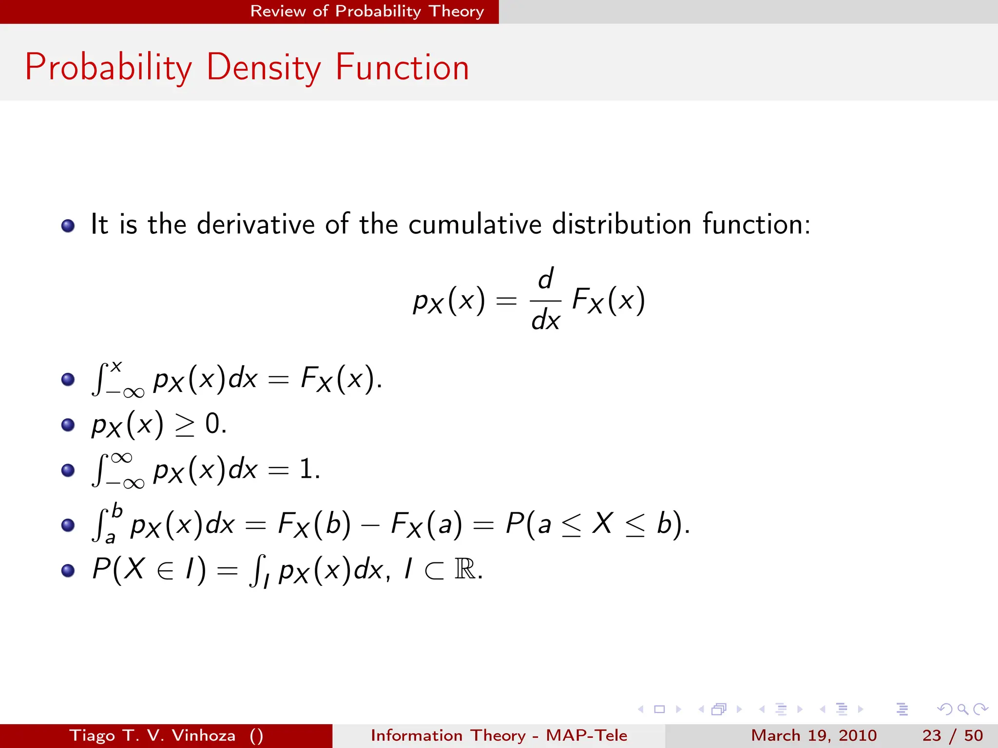
Cumulative Distribution Function
FX : R → [0, 1]
X → FX (x) = P(X ≤ x) = P(ω|X(ω) ≤ x)
FX (∞) = 1
FX (−∞) = 0
If x1 < x2, FX (x2) ≥ FX (x1).
FX (x+) = limϵ→0 FX (x + ϵ) = FX (x). (continuous on the right side).
FX (x) − FX (x−) = P(X = x).
Tiago T. V. Vinhoza () Information Theory - MAP-Tele March 19, 2010 20 / 50](https://image.slidesharecdn.com/principleofinformationtheoryppt-240203141116-479b963e/75/Principle-of-Information-Theory-PkPT-pdf-20-2048.jpg)
![. . . . . .
Review of Probability Theory
Discrete Random Variables
Let us now focus only on discrete random variables.
Let X be a random variable with sample space X
The probability mass function (probability distribution function) of X
is a mapping pX (x) : X → [0, 1] satisfying:
∑
X∈X
pX (x) = 1
The number pX (x) := P(X = x)
Tiago T. V. Vinhoza () Information Theory - MAP-Tele March 19, 2010 24 / 50](https://image.slidesharecdn.com/principleofinformationtheoryppt-240203141116-479b963e/75/Principle-of-Information-Theory-PkPT-pdf-24-2048.jpg)
![. . . . . .
Review of Probability Theory
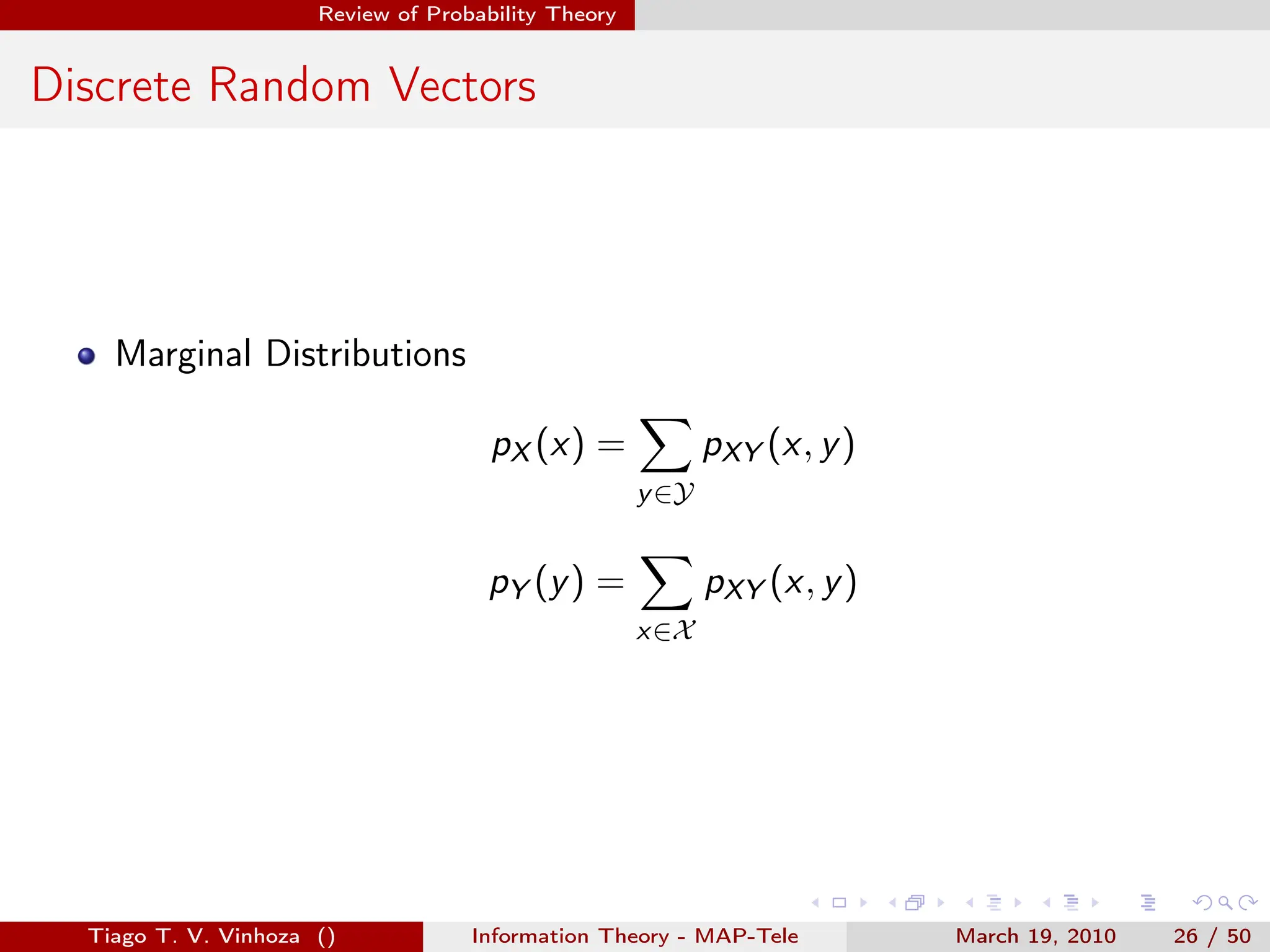
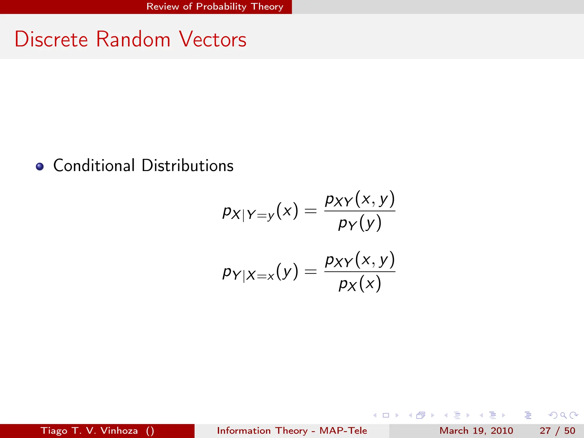
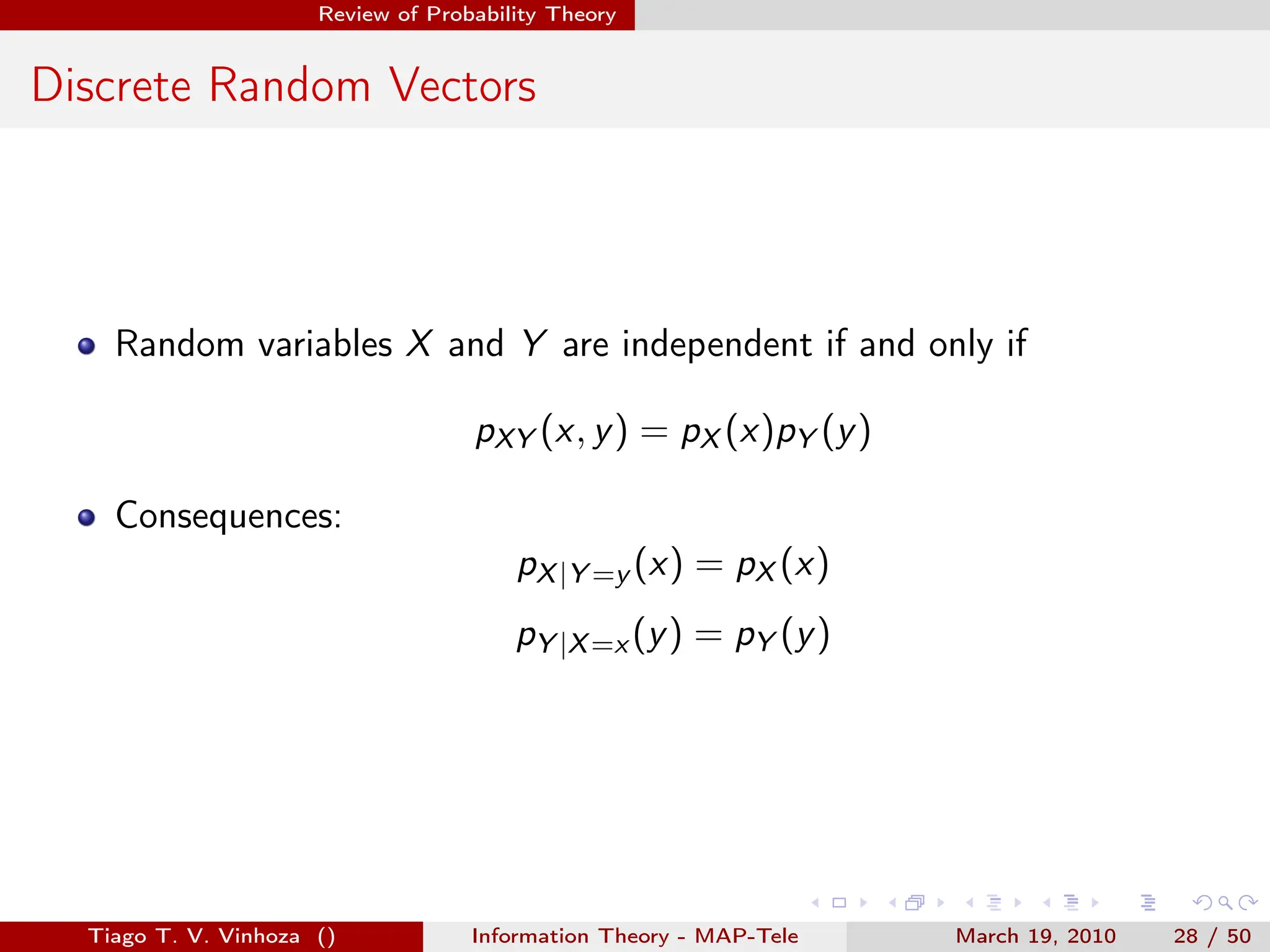
Discrete Random Vectors
Let Z = [X, Y ] be a random vector with sample space Z = X × Y
The joint probability mass function (probability distribution function)
of Z is a mapping pZ (z) : Z → [0, 1] satisfying:
∑
Z∈Z
pZ (z) =
∑
x,y×Y
pXY (x, y) = 1
The number pZ (z) := pXY (x, y) = P(Z = z) = P(X = x, Y = y).
Tiago T. V. Vinhoza () Information Theory - MAP-Tele March 19, 2010 25 / 50](https://image.slidesharecdn.com/principleofinformationtheoryppt-240203141116-479b963e/75/Principle-of-Information-Theory-PkPT-pdf-25-2048.jpg)
![. . . . . .
Review of Probability Theory
Moments of a Discrete Random Variable
The n−th order moment of a discrete random variable X is defined as:
E[Xn
] =
∑
x∈X
xn
pX (x)
if n = 1, we have the mean of X, mX = E[X].
The m−th order central moment of a discrete random variable X is
defined as:
E[(X − mX )m
] =
∑
x∈X
(x − mX )m
pX (x)
if m = 2, we have the variance of X, σ2
X .
Tiago T. V. Vinhoza () Information Theory - MAP-Tele March 19, 2010 29 / 50](https://image.slidesharecdn.com/principleofinformationtheoryppt-240203141116-479b963e/75/Principle-of-Information-Theory-PkPT-pdf-29-2048.jpg)
![. . . . . .
Review of Probability Theory
Moments of a Discrete Random Vector
The joint moment n−th order with relation to X and k−th order with
relation to Y :
mnk = E[Xn
Y k
] =
∑
x∈X
∑
y∈Y
xn
yk
pXY (x, y)
The joint central n−th order with relation to X and k−th order with
relation to Y :
µnk = E[(X−mX )n
(Y −mY )k
] ==
∑
x∈X
∑
y∈Y
(x−mX )n
(y−mY )k
pXY (x, y)
Tiago T. V. Vinhoza () Information Theory - MAP-Tele March 19, 2010 30 / 50](https://image.slidesharecdn.com/principleofinformationtheoryppt-240203141116-479b963e/75/Principle-of-Information-Theory-PkPT-pdf-30-2048.jpg)
![. . . . . .
Review of Probability Theory
Correlation and Covariance
The correlation of two random variables X and Y is the expected value
of their product (joint moment of order 1 in X and order 1 in Y ):
Corr(X, Y ) = m11 = E[XY ]
The covariance of two random variables X and Y is the joint central
moment of order 1 in X and order 1 in Y:
Cov(X, Y ) = µ11 = E[(X − mX )(Y − mY )]
Cov(X, Y ) = Corr(X, Y ) − mX mY
Correlation Coefficient:
ρXY =
Cov(X, Y )
σX σY
→ −1 ≤ ρXY ≤ 1
Tiago T. V. Vinhoza () Information Theory - MAP-Tele March 19, 2010 31 / 50](https://image.slidesharecdn.com/principleofinformationtheoryppt-240203141116-479b963e/75/Principle-of-Information-Theory-PkPT-pdf-31-2048.jpg)
![. . . . . .
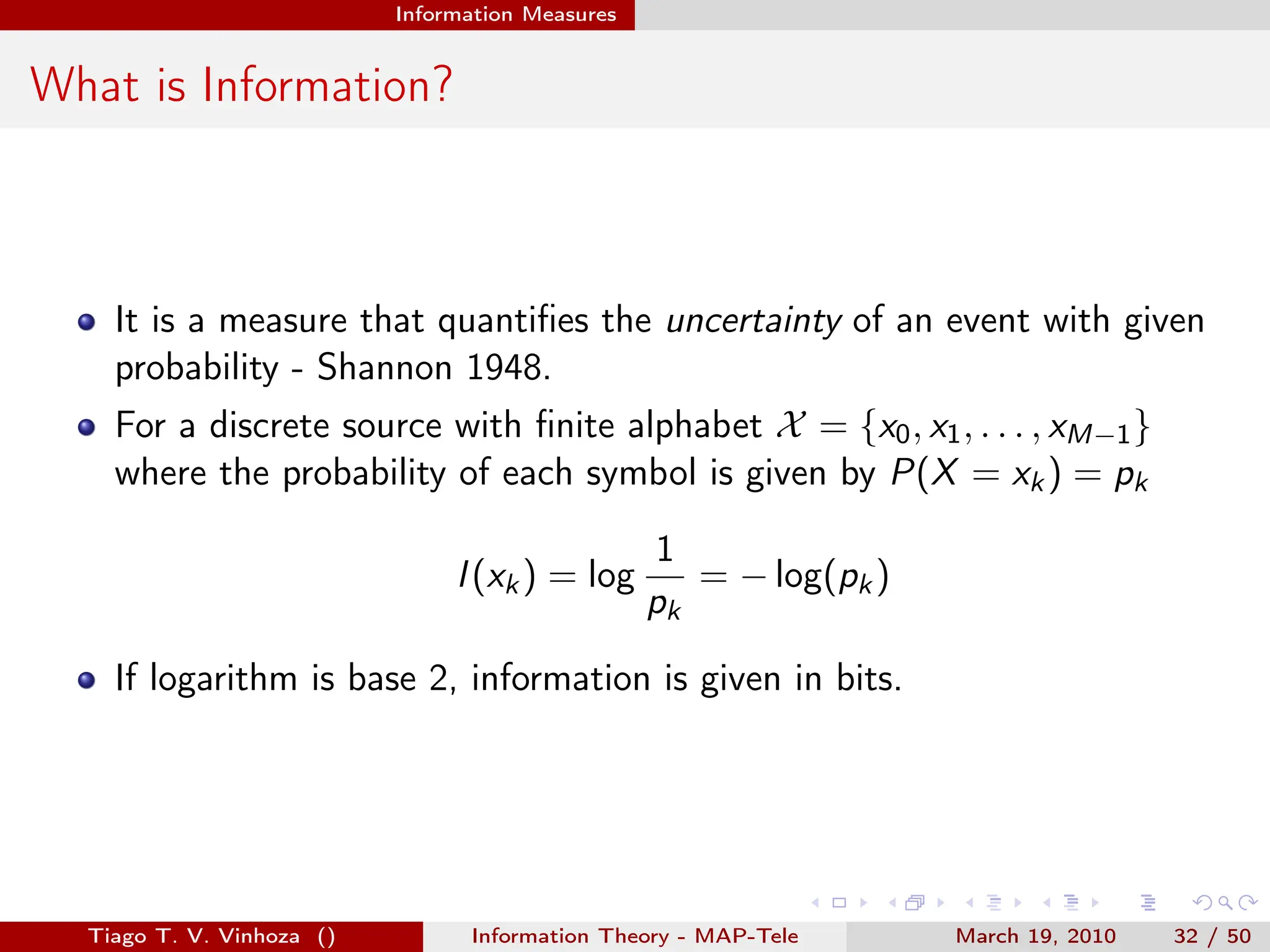
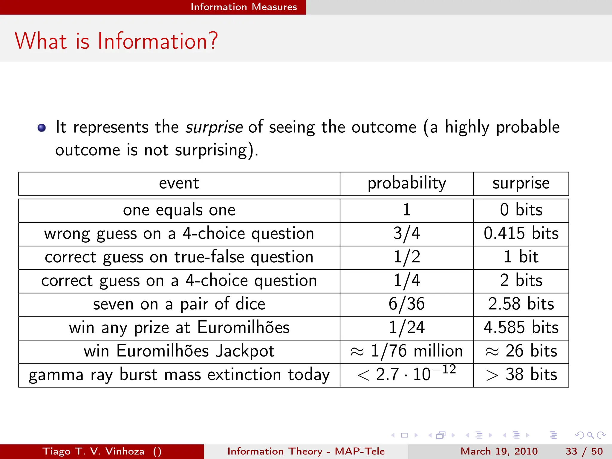
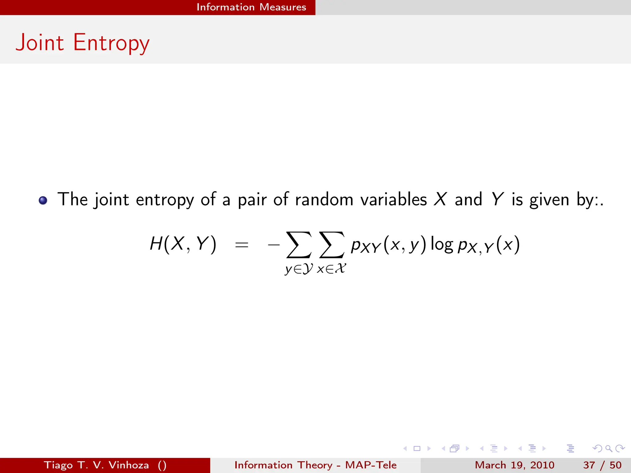
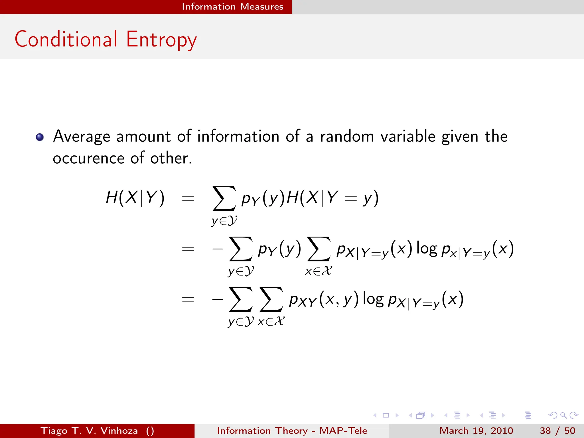
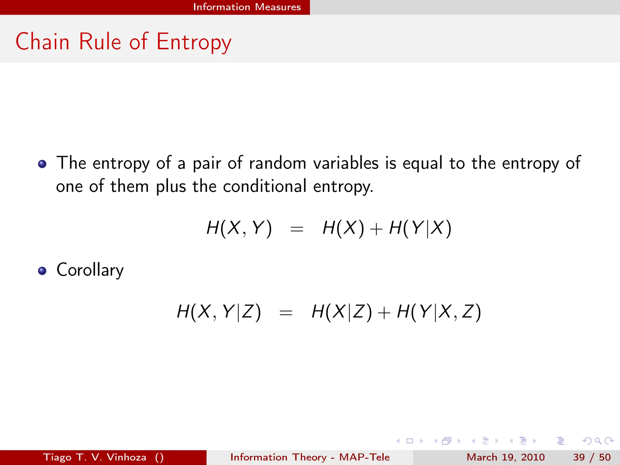
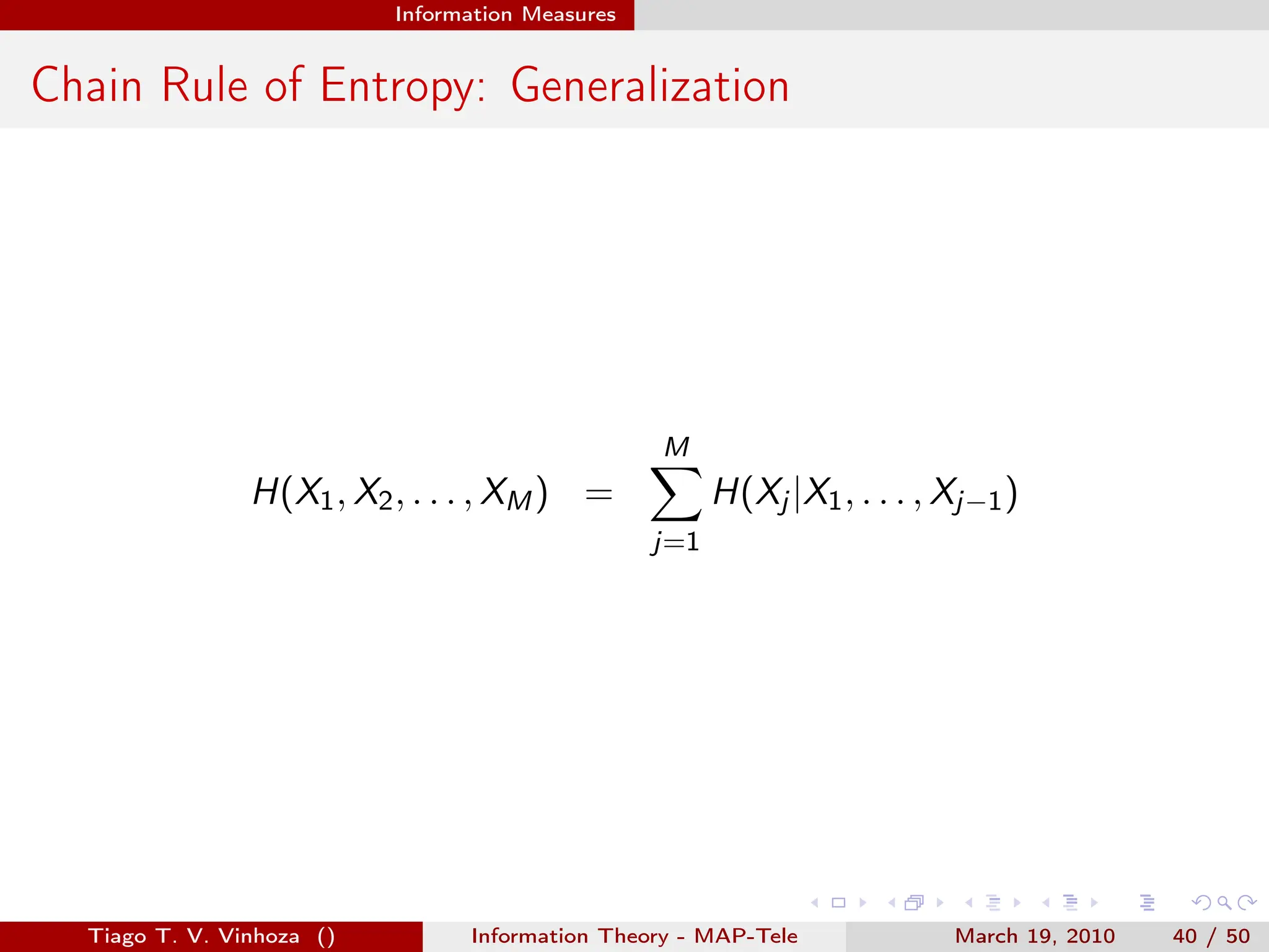
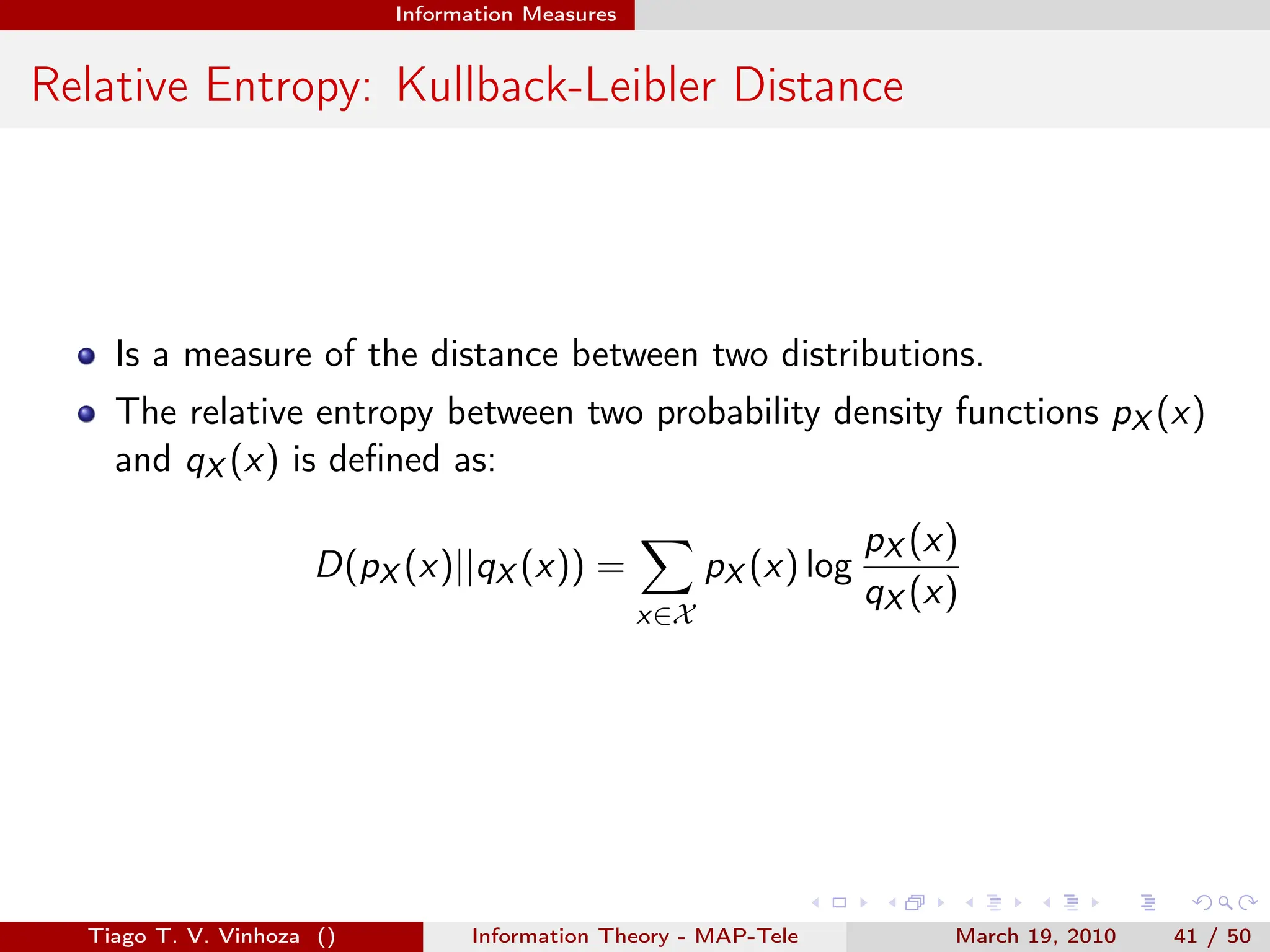
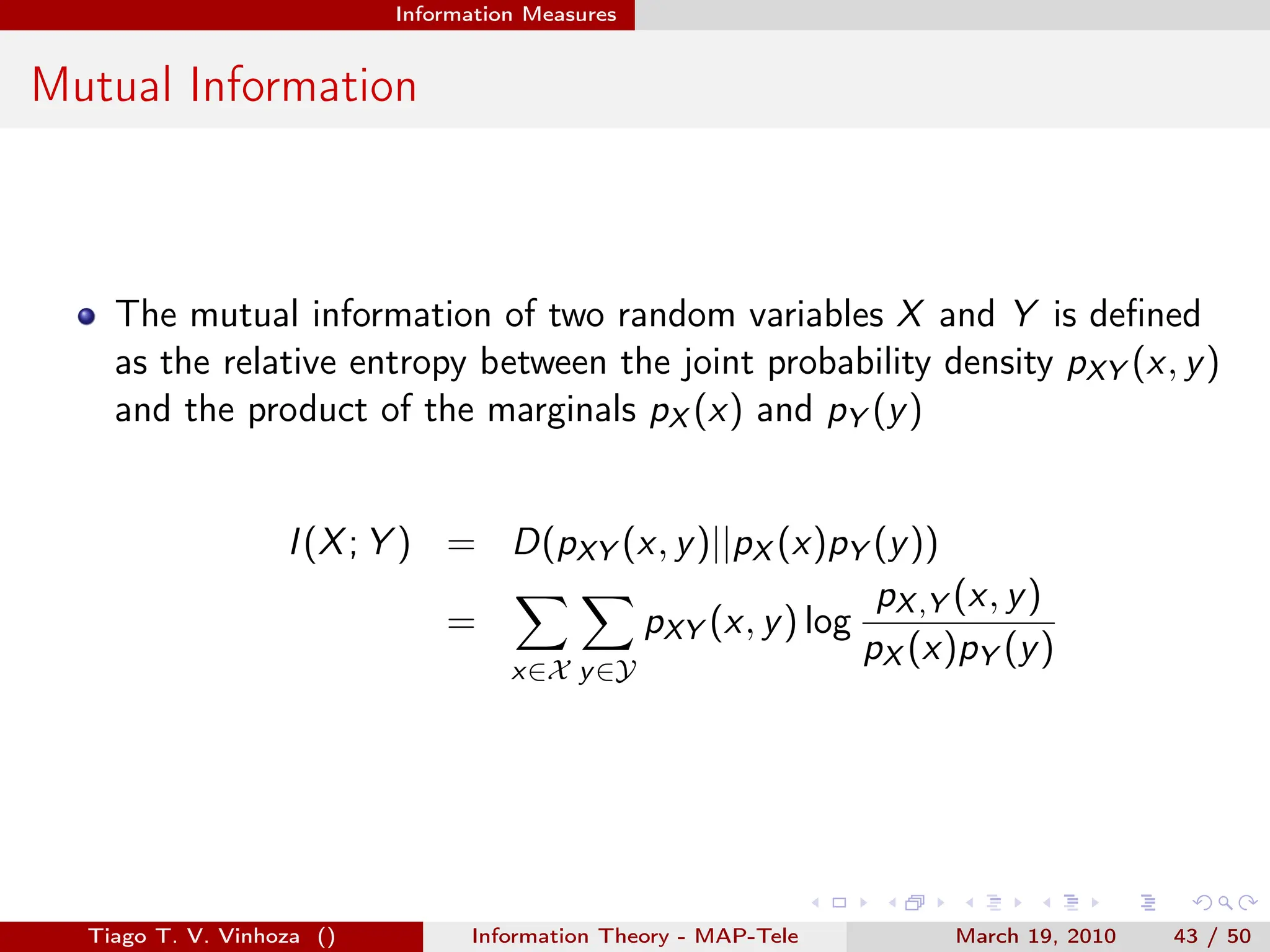
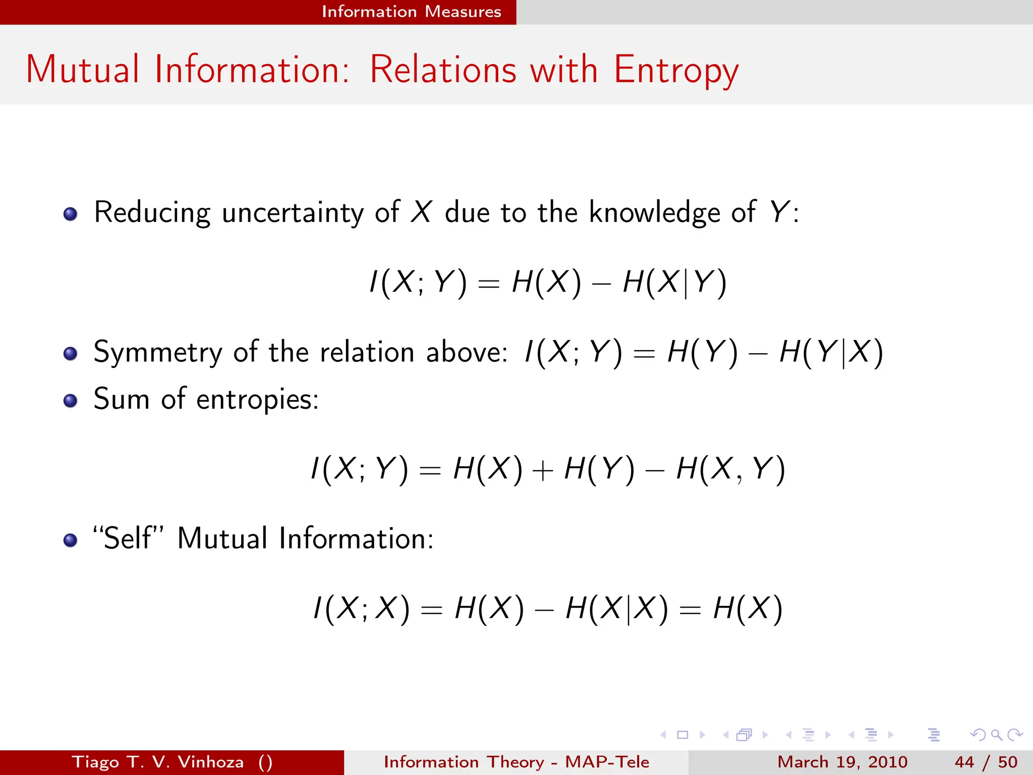
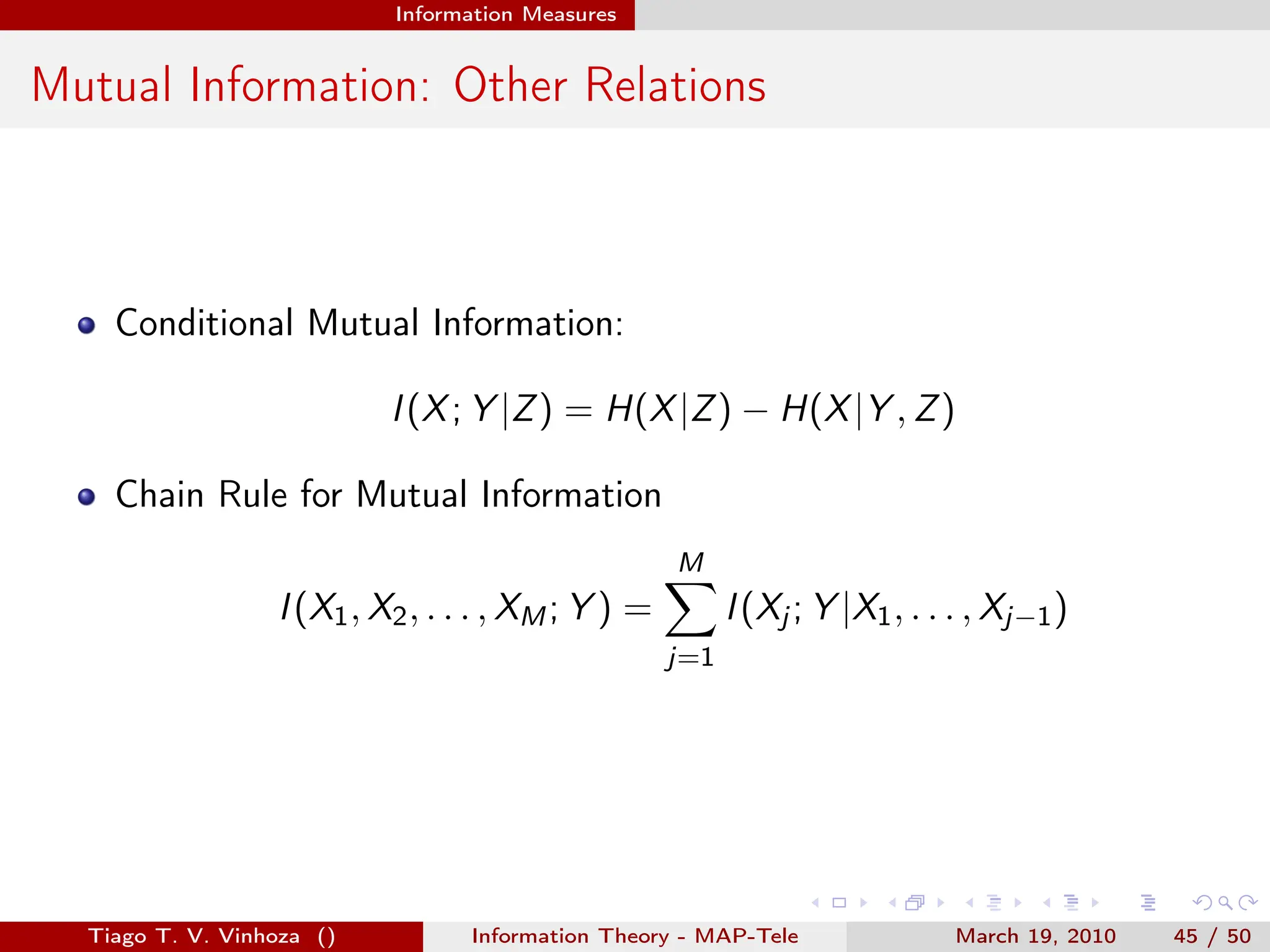
Information Measures
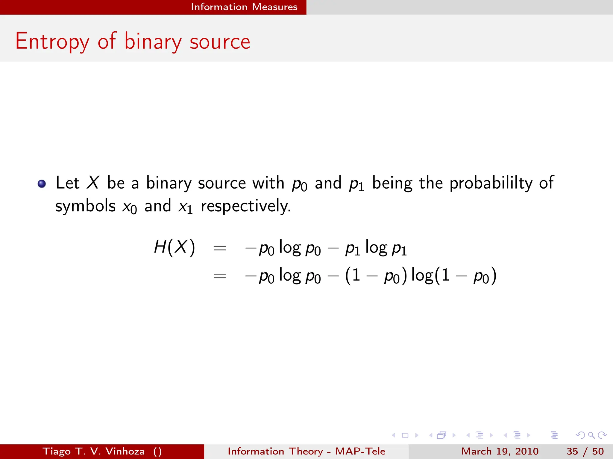
Entropy
Expected value of information from a source.
H(X) = E[I(xk)] =
∑
x∈X
px (x)I(xk)
= −
∑
x∈X
px (x) log px (x)
Tiago T. V. Vinhoza () Information Theory - MAP-Tele March 19, 2010 34 / 50](https://image.slidesharecdn.com/principleofinformationtheoryppt-240203141116-479b963e/75/Principle-of-Information-Theory-PkPT-pdf-34-2048.jpg)

![. . . . . .
Information Measures
Convex and Concave Functions
A function f (·) is convex over ain interval (a, b) if for every
x1, x2 ∈ [a, b] and 0 ≤ λ ≤ 1, if :
f (λx1 + (1 − λ)x2) ≤ λf (x1) + (1 − λ)f (x2)
A function f (·) is convex over an interval (a, b) if its second derivative
is non-negative over that interval (a, b).
A function f (·) is concave if −f (·) is convex.
Examples of convex functions: x2, |x|, ex , x log x, x ≥ 0.
Examples of concave functions: log x and
√
x, for x ≥ 0.
Tiago T. V. Vinhoza () Information Theory - MAP-Tele March 19, 2010 46 / 50](https://image.slidesharecdn.com/principleofinformationtheoryppt-240203141116-479b963e/75/Principle-of-Information-Theory-PkPT-pdf-46-2048.jpg)
![. . . . . .
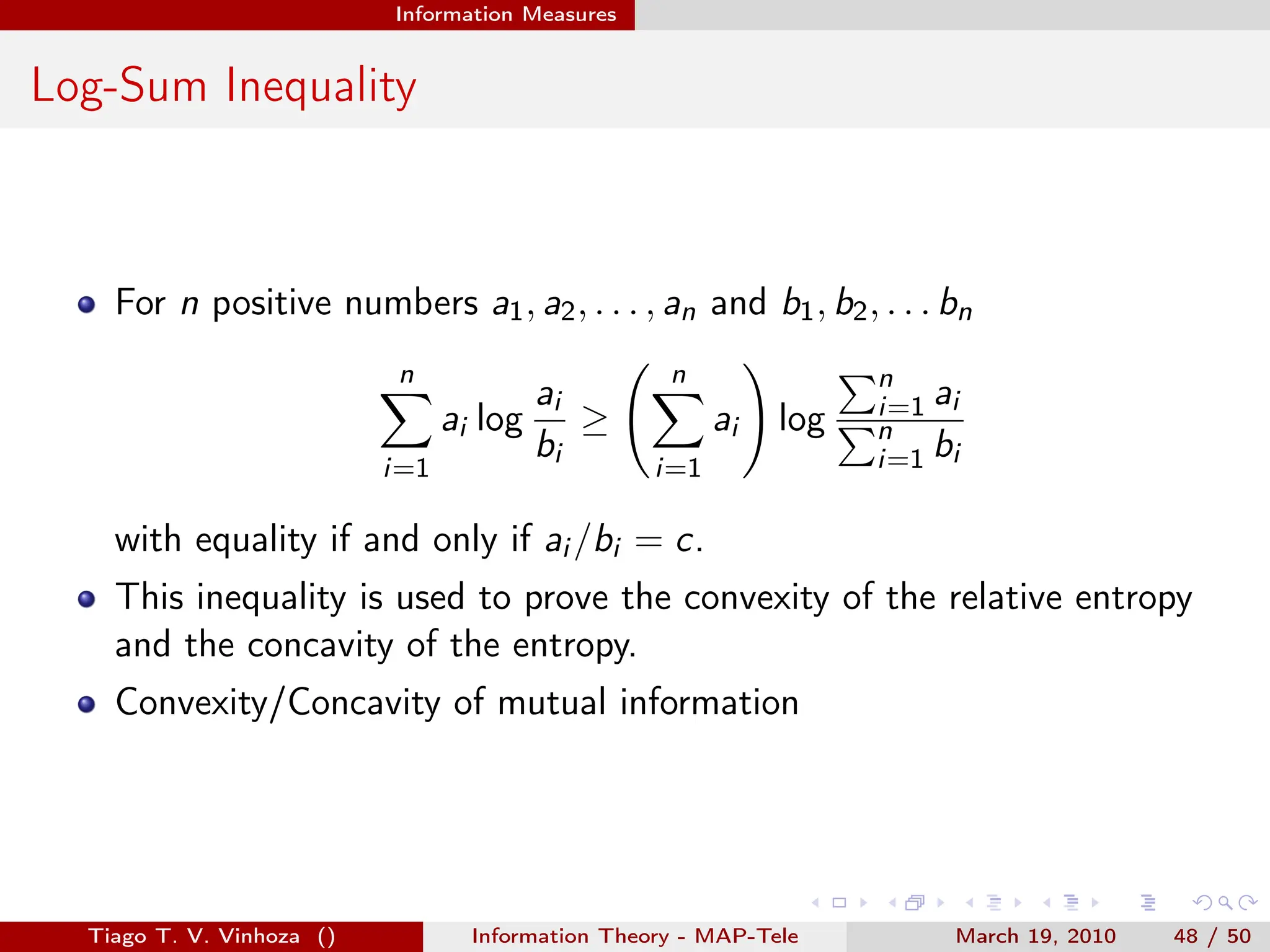
Information Measures
Jensen’s Inequality
If f (·) is a convex function and X is a random variable
E[f (X)] ≥ f (E[X])
Used to show that relative entropy and mutual information are greater
than zero.
Used also to show that H(X) ≤ log |X|.
Tiago T. V. Vinhoza () Information Theory - MAP-Tele March 19, 2010 47 / 50](https://image.slidesharecdn.com/principleofinformationtheoryppt-240203141116-479b963e/75/Principle-of-Information-Theory-PkPT-pdf-47-2048.jpg)