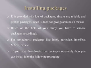
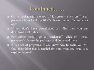
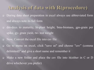
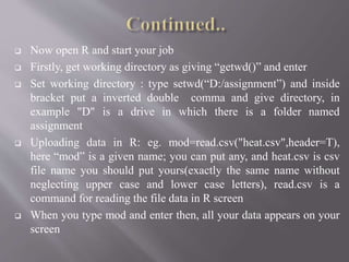
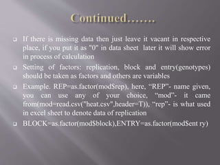
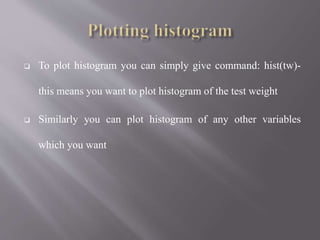
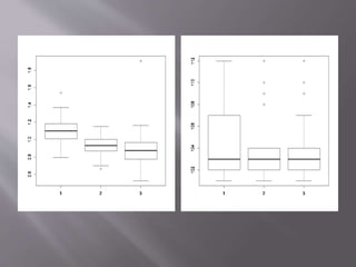
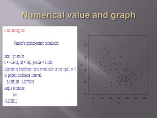
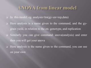
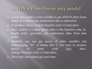
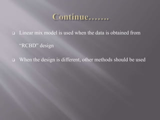
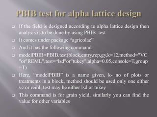
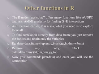
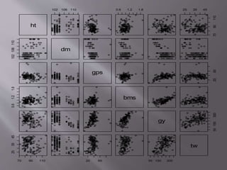
Prepared by: Krishna Dhakal
Academic level: M.Sc.Ag
Department : Genetics and Plant Breeding
Date of final work: March 2, 2016
Agriculture and Forestry University,
Chitwan, Nepal
krishnadhakal19@gmail.com
 It is an elegant, object-oriented programming language
R is an integrated suite of software facilities for data
manipulation, simulation, calculation and graphical display
 It handles and analyzes data very effectively and it contains
a suite of operators for calculations on arrays and matrices
 R is available in Windows and Macintosh versions, as well
as in various flavors of Unix and Linux
 It is currently maintained by the R Core development team – a
hard-working, international group of volunteer developers
 The R project web page is http://www.r-project.org
 For downloading the software directly
 Go to http://cran.us.r-project.org/
 The R project was started by Robert Gentleman and Ross Ihaka
(that’s where the name “R” is derived) from the Statistics
Department in the University of Auckland in 1995
 It has a limited graphical interface (S-Plus has a good one).
This means, it can be harder to learn at the outset
 The command language is a programming language so
students must learn to appreciate syntax issues etc.
 First of all download the latest version of R(zip file)
 Install in your PC
 And the icon of R will appear on your desktop
 Double click on it………….
 When R is started, the program’s “Gui” (graphical user
interface) window appears
 Under the opening message in the R Console is the > (“greater
than”) prompt
 At the > prompt, you tell R what you want it to do
 You give R a command and R does the work and gives the
answer
 If your command is too long to fit on a line or if you submit
an incomplete command, a “+” is used for the continuation
prompt
 To quit R, type q() or use the Exit option in the File menu
 While typing instructions in R, you can save yourself a lot of
typing when you learn to use the arrow keys effectively
 Each command you submit is stored in the History and the up
arrow (↑) will navigate backwards along this history and the
down arrow (↓) forwards
 The left (←) and right arrow (→) keys move backwards and
forwards along the command line
 These keys combined with the mouse for copying,
cutting/pasting can make it very easy to edit and execute
previous commands
 All variables or “objects” created in R are stored in what’s
called the workspace
 To see what variables are in the workspace, you can use the
function ls() to list them (this function doesn’t need any
argument between the parentheses)
 To remove objects from the workspace (you’ll want to do this
occasionally when your workspace gets too cluttered), use the
rm() function
 In Windows, you can clear the entire workspace via the
“Remove all objects” option under the “Misc” menu
 When exiting R, the software asks if you would like to save
your workspace image
 If you click yes, all objects (both new ones created in the
current session and others from earlier sessions) will be
available during your next session
 If you click no, all new objects will be lost and the
workspace will be restored to the last time the image was
saved
 Get in the habit of saving your work – it will probably help
you in the future
 R is provided with lots of packages, always use reliable and
proven packages, since R does not give guarantee on misuse
 Based on the field of your study you have to choose
packages accordingly
 For agriculturist packages like lme4, agricolae, lmerTest,
MASS, car etc.
 if you have downloaded the packages separately then you
can install it by the following procedure
 Go to packages(at the top of R screen)- click on “install
packages from local zip files”- choose the zip file and click
open
 If you don’t have downloaded zip files then you can
download it all online
 For online install- go to “packages”- click on “install
packages”- choose the packages and download them
 R is a sea of programs, if you know how to swim you will
find everything that is needed for you, what you need is to
explore yourself
 During data sheet preparation in excel always use abbreviated form
and always note its full form
 dm-days to maturity, ht-plant height, bms-biomass, gps-grain per
spike, gy- grain yield, tw- test weight
 Now, Convert the excel file into csv file
 Go to menu on excel, click "save as" and choose "csv” (comma
delimited)" and give a short name and remember it
 Make a new folder and place the csv file into it(either in C or D
drive whichever you prefer)
 Now open R and start your job
 Firstly, get working directory as giving “getwd()” and enter
 Set working directory : type setwd(“D:/assignment”) and inside
bracket put a inverted double comma and give directory, in
example "D" is a drive in which there is a folder named
assignment
 Uploading data in R: eg. mod=read.csv("heat.csv",header=T),
here “mod” is a given name; you can put any, and heat.csv is csv
file name you should put yours(exactly the same name without
neglecting upper case and lower case letters), read.csv is a
command for reading the file data in R screen
 When you type mod and enter then, all your data appears on your
screen
 If there is missing data then just leave it vacant in respective
place, if you put it as "0" in data sheet later it will show error
in process of calculation
 Setting of factors: replication, block and entry(genotypes)
should be taken as factors and others are variables
 Example. REP=as.factor(mod$rep), here, “REP”- name given,
you can use any of your choice, “mod”- it came
from(mod=read.csv("heat.csv",header=T)), “rep”- is what used
in excel sheet to denote data of replication
 BLOCK=as.factor(mod$block),ENTRY=as.factor(mod$ent ry)
 yield, height, biomass, grain per spike, test weight etc. are
variables, in these cases what we do is: HT=(mod$ht),
DM=(mod$dm), GPS=(mod$gps), BMS=(mod$bms),
GY=(mod$gy), TW=(mod$tw)
 Making of data frame: example,
Data=data.frame(REP,BLOCK,ENTRY,HT,DM,GPS,BMS,
GY,TW)
 Always use the exact names that you have given to the
respective factors and variables
 To get summary of your data, perform “summary(data)” and
press “enter”
 Data summary will give you the mean, median, and quartiles
values
 Qqplot is required to find the distribution of data of a particular
variable
 It helps us to find the extreme outliers
 For qqPlot , package “car” is required to install
 After installation of “car”, give command: require(car) then enter
 QqPlot also requires package “lme4” and “lmerTest”
 Now, mod=lmer(gy~entry+(1|rep),data)
 Then qqPlot(resid(mod)) then enter
 You will see the picture on your screen
-2 -1 0 1 2
-10-5051015
norm quantiles
resid(mod.ht)
-2 -1 0 1 2
-20-10010203040
norm quantiles
resid(mod.gps)
 The process is same as in qqPlot
 The only difference is you give command like
:plot(resid(mod.ht)) for getting extreme outliers in height
 Similarly, you can get outliers in other data just by
interchanging the command name
 In screen you will see the extreme outliers with their
respective entry number
0.00 0.05 0.10 0.15 0.20 0.25 0.30 0.35
-4-2024
Leverage
Standardizedresiduals
lm(dm~entry+rep)
Cook'sdistance
ResidualsvsLeverage
78
77
42
 To plot histogram you can simply give command: hist(tw)-
this means you want to plot histogram of the test weight
 Similarly you can plot histogram of any other variables
which you want
 To produce box plot you can simply perform:
boxplot(gy~rep)
 Here the box plot will show the result of grain yield with
respect to the replication
 Box plot generally have 5 components the tail regions gives
two extreme values the middle line inside the box gives
median or Q2 value, top part of box shows Q1, bottom part
shows Q3
 To find out the correlation between the yield and other
variables: cor.test(gy,tw) or any other which you want
 Correlation test gives you the value with either positive or
negative correlation
50 100 150 200 250 300 350
708090100110
gy
ht
 It is used to see the normality of the variables
 Shapiro.test(tw), shapiro.test(gy) etc.
 In this model: eg. analysis=lm(gy~en+rep,data)
 Here analysis is a name given to the command, and the gy-
grain yield, in relation to the en- genotype, and replication
 Similarly you can give command: anova(analysis) and enter
then you will get your anova
 Here analysis is the name given to the command, you can use
on your own
 Linear mix model is more reliable to get ANOVA then linear
model as it reduces the randomness due to replication
 To produce anova: mod.ht=lmer(ht~entry+(1|rep),data)
 Here, mod.ht is a name given, lmer is the function code, ht-
height, entry- genotype, rep- replication, data- from data
frame
 Similarly you can get anova of other variables just
interchanging “ht”. It means that if you want to produce
anova of grain yield (gy) then,:
mod.gy=lmer(gy~entry+(1|rep),data)
 Then type: anova(mod.gy) and enter
 Linear mix model is used when the data is obtained from
“RCBD” design
 When the design is different, other methods should be used
 If the field is designed according to alpha lattice design then
analysis is to be done by using PBIB test
 It comes under package “agricolae”
 And it has the following command
 modelPBIB=PBIB.test(block,entry,rep,gy,k=12,method="VC
"or"REML",test=“lsd"or"tukey",alpha=0.05,console=T,group
=T)
 Here, “modelPBIB” is a name given, k- no of plots or
treatments in a block, method should be used only one either
vc or reml, test may be either lsd or tukey
 This command is for grain yield, similarly you can find the
value for other variables
 The R under “agricolae” offers many functions like AUDPC
analysis, AMMI analysis- for finding G×E interactions
 As I mention earlier, R is a sea, what you need is to explore
these all
 To find correlation directly from data frame you just remove
the factors and retain only the variables
 Eg. data=data.frame (rep,entry,block,gy,ht,dm,tw,bms)
 Remove rep, entry, block :
data=data.frame(ht,dm,bms,gy,tw)
 Now give command: plot(data) and enter you will see the
corrrelation
ht
102 106 110 0.6 1.2 1.8 25 35 45
7090110
102106110
dm
gps
2060
0.61.21.8
bms
gy
50150300
70 90 110
253545
20 60 50 150 300
tw
After climbing a great hill,
one only finds that there are
many more hills to climb.
Nelson Mandela
Presentation on use of r statistics

Presentation on use of r statistics

  • 1.
    Prepared by: KrishnaDhakal Academic level: M.Sc.Ag Department : Genetics and Plant Breeding Date of final work: March 2, 2016 Agriculture and Forestry University, Chitwan, Nepal krishnadhakal19@gmail.com
  • 2.
     It isan elegant, object-oriented programming language R is an integrated suite of software facilities for data manipulation, simulation, calculation and graphical display  It handles and analyzes data very effectively and it contains a suite of operators for calculations on arrays and matrices  R is available in Windows and Macintosh versions, as well as in various flavors of Unix and Linux
  • 3.
     It iscurrently maintained by the R Core development team – a hard-working, international group of volunteer developers  The R project web page is http://www.r-project.org  For downloading the software directly  Go to http://cran.us.r-project.org/  The R project was started by Robert Gentleman and Ross Ihaka (that’s where the name “R” is derived) from the Statistics Department in the University of Auckland in 1995
  • 4.
     It hasa limited graphical interface (S-Plus has a good one). This means, it can be harder to learn at the outset  The command language is a programming language so students must learn to appreciate syntax issues etc.
  • 5.
     First ofall download the latest version of R(zip file)  Install in your PC  And the icon of R will appear on your desktop  Double click on it………….
  • 7.
     When Ris started, the program’s “Gui” (graphical user interface) window appears  Under the opening message in the R Console is the > (“greater than”) prompt  At the > prompt, you tell R what you want it to do
  • 8.
     You giveR a command and R does the work and gives the answer  If your command is too long to fit on a line or if you submit an incomplete command, a “+” is used for the continuation prompt  To quit R, type q() or use the Exit option in the File menu
  • 9.
     While typinginstructions in R, you can save yourself a lot of typing when you learn to use the arrow keys effectively  Each command you submit is stored in the History and the up arrow (↑) will navigate backwards along this history and the down arrow (↓) forwards  The left (←) and right arrow (→) keys move backwards and forwards along the command line  These keys combined with the mouse for copying, cutting/pasting can make it very easy to edit and execute previous commands
  • 10.
     All variablesor “objects” created in R are stored in what’s called the workspace  To see what variables are in the workspace, you can use the function ls() to list them (this function doesn’t need any argument between the parentheses)  To remove objects from the workspace (you’ll want to do this occasionally when your workspace gets too cluttered), use the rm() function  In Windows, you can clear the entire workspace via the “Remove all objects” option under the “Misc” menu
  • 11.
     When exitingR, the software asks if you would like to save your workspace image  If you click yes, all objects (both new ones created in the current session and others from earlier sessions) will be available during your next session  If you click no, all new objects will be lost and the workspace will be restored to the last time the image was saved  Get in the habit of saving your work – it will probably help you in the future
  • 12.
     R isprovided with lots of packages, always use reliable and proven packages, since R does not give guarantee on misuse  Based on the field of your study you have to choose packages accordingly  For agriculturist packages like lme4, agricolae, lmerTest, MASS, car etc.  if you have downloaded the packages separately then you can install it by the following procedure
  • 13.
     Go topackages(at the top of R screen)- click on “install packages from local zip files”- choose the zip file and click open  If you don’t have downloaded zip files then you can download it all online  For online install- go to “packages”- click on “install packages”- choose the packages and download them  R is a sea of programs, if you know how to swim you will find everything that is needed for you, what you need is to explore yourself
  • 14.
     During datasheet preparation in excel always use abbreviated form and always note its full form  dm-days to maturity, ht-plant height, bms-biomass, gps-grain per spike, gy- grain yield, tw- test weight  Now, Convert the excel file into csv file  Go to menu on excel, click "save as" and choose "csv” (comma delimited)" and give a short name and remember it  Make a new folder and place the csv file into it(either in C or D drive whichever you prefer)
  • 15.
     Now openR and start your job  Firstly, get working directory as giving “getwd()” and enter  Set working directory : type setwd(“D:/assignment”) and inside bracket put a inverted double comma and give directory, in example "D" is a drive in which there is a folder named assignment  Uploading data in R: eg. mod=read.csv("heat.csv",header=T), here “mod” is a given name; you can put any, and heat.csv is csv file name you should put yours(exactly the same name without neglecting upper case and lower case letters), read.csv is a command for reading the file data in R screen  When you type mod and enter then, all your data appears on your screen
  • 18.
     If thereis missing data then just leave it vacant in respective place, if you put it as "0" in data sheet later it will show error in process of calculation  Setting of factors: replication, block and entry(genotypes) should be taken as factors and others are variables  Example. REP=as.factor(mod$rep), here, “REP”- name given, you can use any of your choice, “mod”- it came from(mod=read.csv("heat.csv",header=T)), “rep”- is what used in excel sheet to denote data of replication  BLOCK=as.factor(mod$block),ENTRY=as.factor(mod$ent ry)
  • 20.
     yield, height,biomass, grain per spike, test weight etc. are variables, in these cases what we do is: HT=(mod$ht), DM=(mod$dm), GPS=(mod$gps), BMS=(mod$bms), GY=(mod$gy), TW=(mod$tw)  Making of data frame: example, Data=data.frame(REP,BLOCK,ENTRY,HT,DM,GPS,BMS, GY,TW)
  • 21.
     Always usethe exact names that you have given to the respective factors and variables  To get summary of your data, perform “summary(data)” and press “enter”  Data summary will give you the mean, median, and quartiles values
  • 22.
     Qqplot isrequired to find the distribution of data of a particular variable  It helps us to find the extreme outliers  For qqPlot , package “car” is required to install  After installation of “car”, give command: require(car) then enter  QqPlot also requires package “lme4” and “lmerTest”  Now, mod=lmer(gy~entry+(1|rep),data)  Then qqPlot(resid(mod)) then enter  You will see the picture on your screen
  • 23.
    -2 -1 01 2 -10-5051015 norm quantiles resid(mod.ht) -2 -1 0 1 2 -20-10010203040 norm quantiles resid(mod.gps)
  • 24.
     The processis same as in qqPlot  The only difference is you give command like :plot(resid(mod.ht)) for getting extreme outliers in height  Similarly, you can get outliers in other data just by interchanging the command name  In screen you will see the extreme outliers with their respective entry number
  • 25.
    0.00 0.05 0.100.15 0.20 0.25 0.30 0.35 -4-2024 Leverage Standardizedresiduals lm(dm~entry+rep) Cook'sdistance ResidualsvsLeverage 78 77 42
  • 26.
     To plothistogram you can simply give command: hist(tw)- this means you want to plot histogram of the test weight  Similarly you can plot histogram of any other variables which you want
  • 28.
     To producebox plot you can simply perform: boxplot(gy~rep)  Here the box plot will show the result of grain yield with respect to the replication  Box plot generally have 5 components the tail regions gives two extreme values the middle line inside the box gives median or Q2 value, top part of box shows Q1, bottom part shows Q3
  • 30.
     To findout the correlation between the yield and other variables: cor.test(gy,tw) or any other which you want  Correlation test gives you the value with either positive or negative correlation
  • 31.
    50 100 150200 250 300 350 708090100110 gy ht
  • 32.
     It isused to see the normality of the variables  Shapiro.test(tw), shapiro.test(gy) etc.
  • 33.
     In thismodel: eg. analysis=lm(gy~en+rep,data)  Here analysis is a name given to the command, and the gy- grain yield, in relation to the en- genotype, and replication  Similarly you can give command: anova(analysis) and enter then you will get your anova  Here analysis is the name given to the command, you can use on your own
  • 34.
     Linear mixmodel is more reliable to get ANOVA then linear model as it reduces the randomness due to replication  To produce anova: mod.ht=lmer(ht~entry+(1|rep),data)  Here, mod.ht is a name given, lmer is the function code, ht- height, entry- genotype, rep- replication, data- from data frame  Similarly you can get anova of other variables just interchanging “ht”. It means that if you want to produce anova of grain yield (gy) then,: mod.gy=lmer(gy~entry+(1|rep),data)  Then type: anova(mod.gy) and enter
  • 35.
     Linear mixmodel is used when the data is obtained from “RCBD” design  When the design is different, other methods should be used
  • 36.
     If thefield is designed according to alpha lattice design then analysis is to be done by using PBIB test  It comes under package “agricolae”  And it has the following command  modelPBIB=PBIB.test(block,entry,rep,gy,k=12,method="VC "or"REML",test=“lsd"or"tukey",alpha=0.05,console=T,group =T)  Here, “modelPBIB” is a name given, k- no of plots or treatments in a block, method should be used only one either vc or reml, test may be either lsd or tukey  This command is for grain yield, similarly you can find the value for other variables
  • 38.
     The Runder “agricolae” offers many functions like AUDPC analysis, AMMI analysis- for finding G×E interactions  As I mention earlier, R is a sea, what you need is to explore these all  To find correlation directly from data frame you just remove the factors and retain only the variables  Eg. data=data.frame (rep,entry,block,gy,ht,dm,tw,bms)  Remove rep, entry, block : data=data.frame(ht,dm,bms,gy,tw)  Now give command: plot(data) and enter you will see the corrrelation
  • 39.
    ht 102 106 1100.6 1.2 1.8 25 35 45 7090110 102106110 dm gps 2060 0.61.21.8 bms gy 50150300 70 90 110 253545 20 60 50 150 300 tw
  • 40.
    After climbing agreat hill, one only finds that there are many more hills to climb. Nelson Mandela