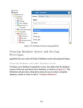
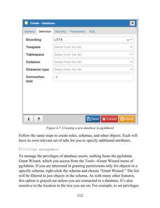
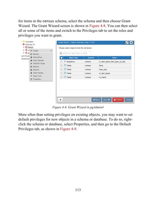
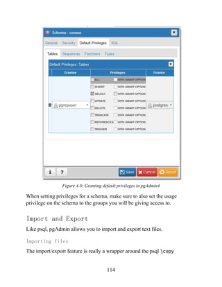
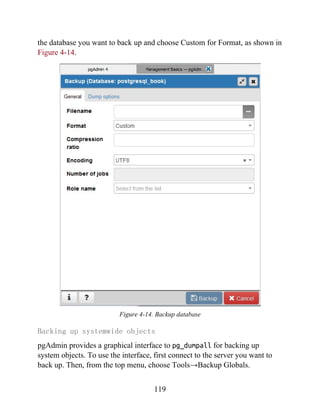
This document provides an overview and introduction to the third edition of the book "PostgreSQL: Up and Running" by Regina O. Obe and Leo S. Hsu. The summary includes a brief description of the book's contents, intended audience, and additional PostgreSQL resources for readers.

![See http://oreilly.com/catalog/errata.csp?isbn=9781491963418 for release
details.
The O’Reilly logo is a registered trademark of O’Reilly Media, Inc.
PostgreSQL: Up and Running, the cover image, and related trade dress are
trademarks of O’Reilly Media, Inc.
While the publisher and the authors have used good faith efforts to ensure
that the information and instructions contained in this work are accurate, the
publisher and the authors disclaim all responsibility for errors or omissions,
including without limitation responsibility for damages resulting from the use
of or reliance on this work. Use of the information and instructions contained
in this work is at your own risk. If any code samples or other technology this
work contains or describes is subject to open source licenses or the
intellectual property rights of others, it is your responsibility to ensure that
your use thereof complies with such licenses and/or rights.
978-1-491-96341-8
[LSI]
4](https://image.slidesharecdn.com/postgresqlupandrunningapracticalguidetotheadvancedopensourcedatabasepdfdrive-221213051845-fb16fe5b/85/PostgreSQL_-Up-and-Running_-A-Practical-Guide-to-the-Advanced-Open-Source-Database-PDFDrive-pdf-4-320.jpg)
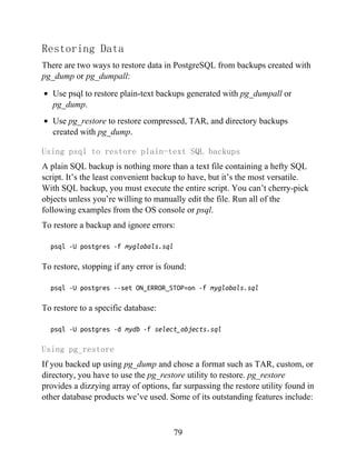
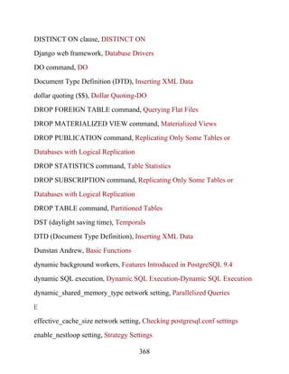
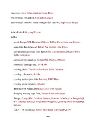
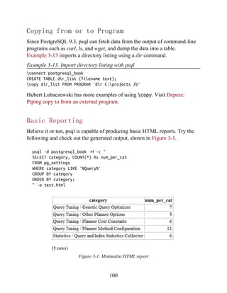
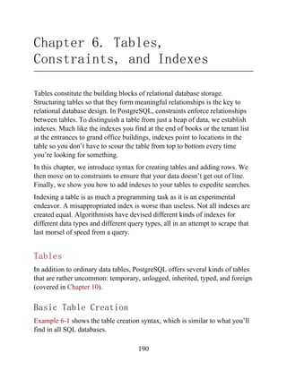
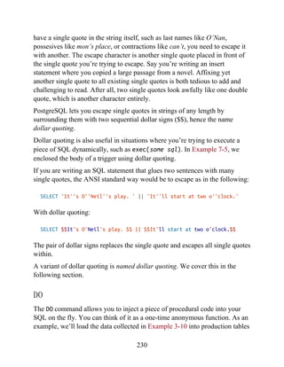
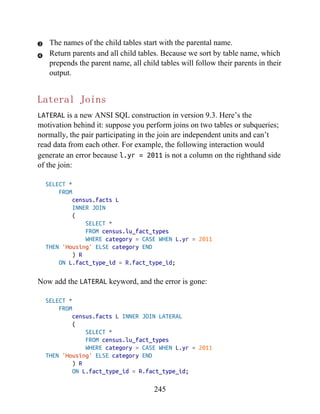
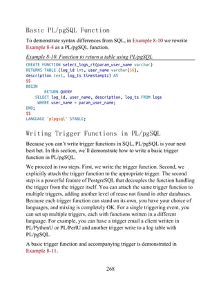
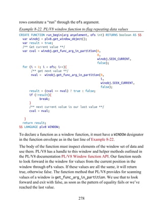
![copy sometable FROM somefile.txt NULL As '';
WARNING
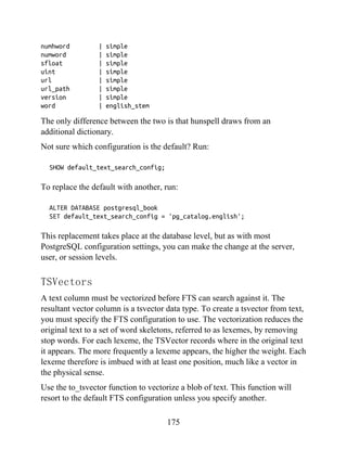
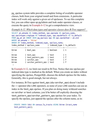
Don’t confuse the copy command in psql with the COPY statement provided by
the SQL language. Because psql is a client utility, all paths are interpreted
relative to the connected client. The SQL copy is server-based and runs under
the context of the postgres service OS account. The input file for an SQL copy
must reside in a path accessible by the postgres service account.
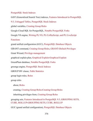
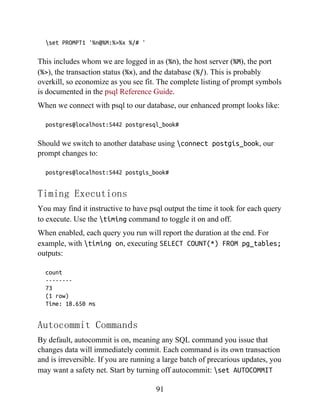
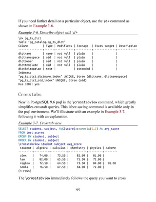
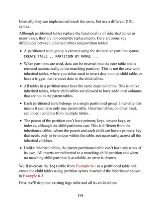
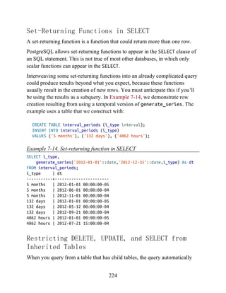
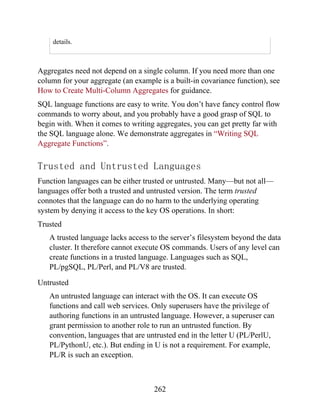
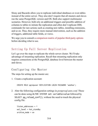
psql Export
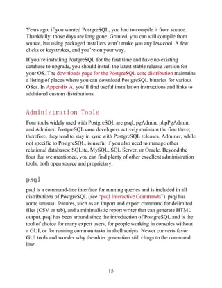
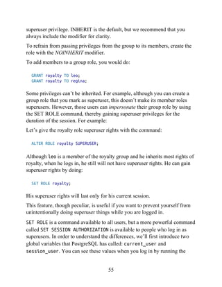
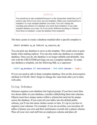
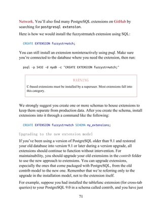
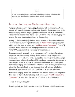
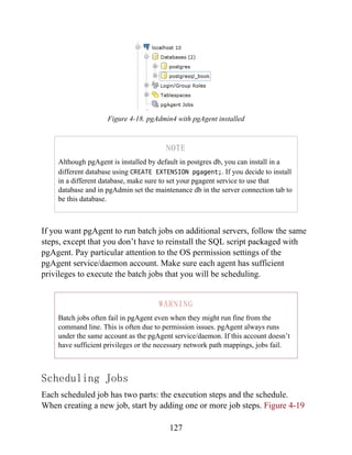
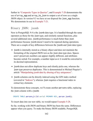
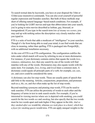
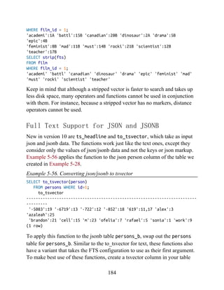
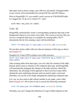
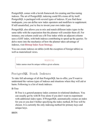
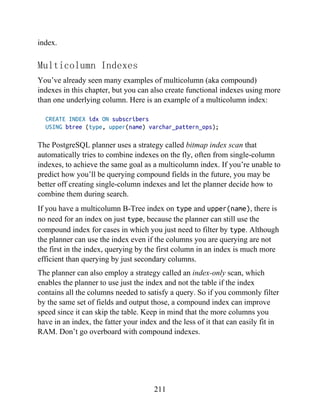
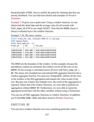
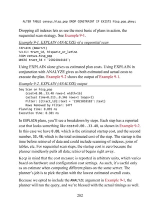
Exporting data is even easier than importing. You can even export selected
rows from a table. Use the psql copy command to export. Example 3-11
demonstrates how to export the data we just loaded back to a tab-delimited
file.
Example 3-11. Exporting data with psql
connect postgresql_book
copy (SELECT * FROM staging.factfinder_import WHERE s01 ~ E'^[0-9]+' )
TO '/test.tab'
WITH DELIMITER E't' CSV HEADER
The default behavior of exporting data without qualifications is to export to a
tab-delimited file. However, the tab-delimited format does not export header
columns. You can use the HEADER option only with the comma-delimited
format (see Example 3-12).
Example 3-12. Exporting data with psql
connect postgresql_book
copy staging.factfinder_import TO '/test.csv'
WITH CSV HEADER QUOTE '"' FORCE QUOTE *
FORCE QUOTE * double quotes all columns. For clarity, we specified the
quoting character even though psql defaults to double quotes.
99](https://image.slidesharecdn.com/postgresqlupandrunningapracticalguidetotheadvancedopensourcedatabasepdfdrive-221213051845-fb16fe5b/85/PostgreSQL_-Up-and-Running_-A-Practical-Guide-to-the-Advanced-Open-Source-Database-PDFDrive-pdf-99-320.jpg)
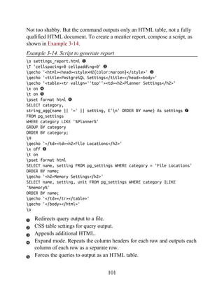
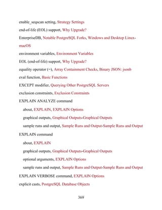
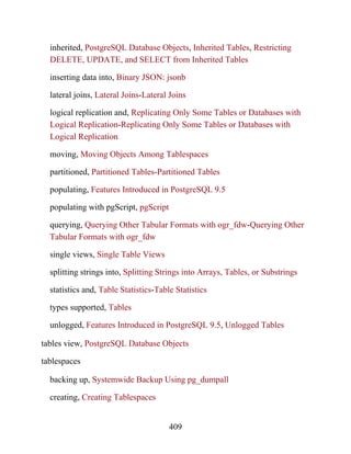
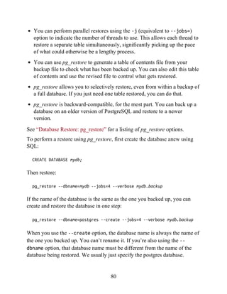
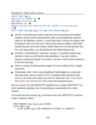
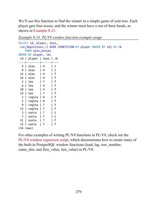
![DECLARE @I, @labels, @tdef;
SET @I = 0;
Labels will hold records.
SET @labels =
SELECT
quote_ident(
replace(
replace(lower(COALESCE(fact_subcats[4],
fact_subcats[3])), ' ', '_')
,':',''
)
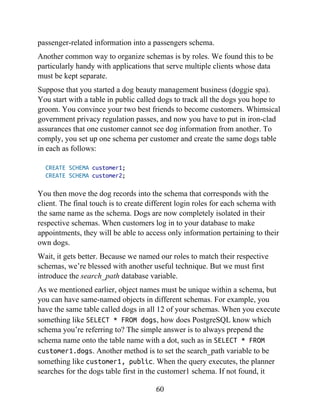
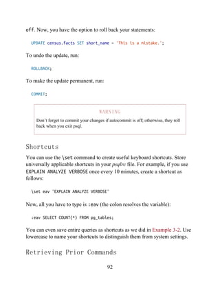
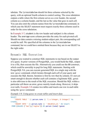
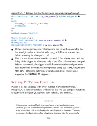
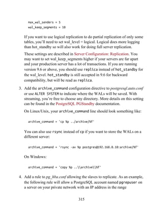
contrast, pgScript commits each SQL insert or update statement as it runs
through the script. This makes pgScript particularly handy for memory-
hungry processes that you don’t need completed as single transactions. After
each transaction commits, memory becomes available for the next one. You
can see an example where we use pgScript for batch geocoding at Using
pgScript for Geocoding.
The pgScript language is lazily typed and supports conditionals, loops, data
generators, basic print statements, and record variables. The general syntax is
similar to that of Transact SQL, the stored procedure language of Microsoft
SQL Server. Variables, prepended with @, can hold scalars or arrays,
including the results of SQL commands. Commands such as DECLARE and
SET, and control constructs such as IF-ELSE and WHILE loops, are part of the
pgScript language.
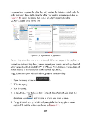
Launch pgScript by opening a regular SQL query window. After typing in
your script, execute it by clicking the pgScript icon ( ).
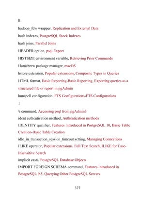
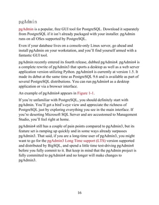
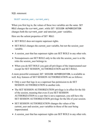
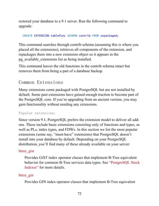
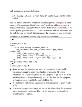
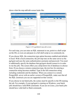
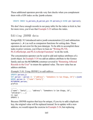
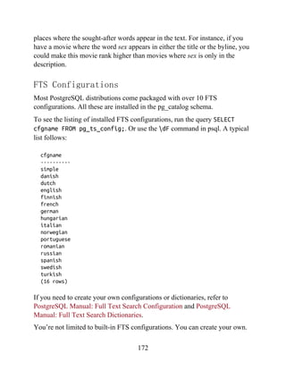
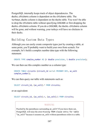
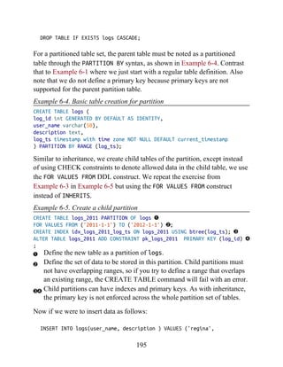
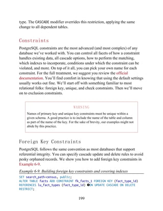
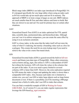
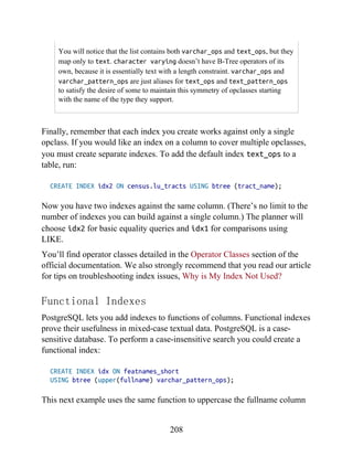
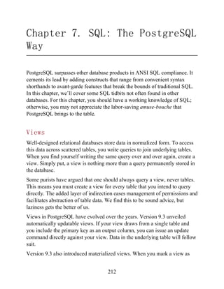
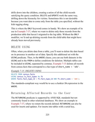
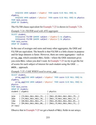
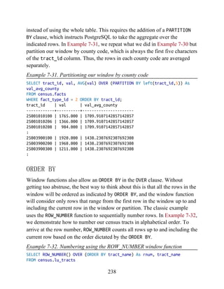
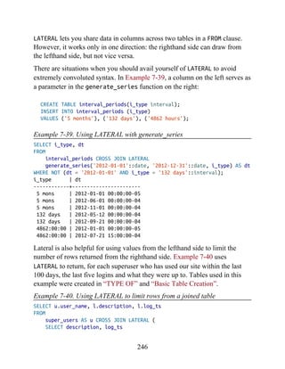
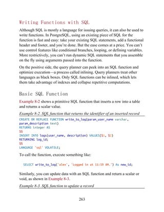
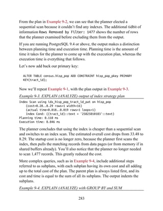
We’ll now show you some examples of pgScripts. Example 4-1 demonstrates
how to use pgScript record variables and loops to build a crosstab table, using
the lu_fact_types table we create in Example 7-22. The pgScript creates an
empty table called census.hisp_pop with numeric columns:
hispanic_or_latino, white_alone,
black_or_african_american_alone, and so on.
Example 4-1. Create a table using record variables in pgScript
122](https://image.slidesharecdn.com/postgresqlupandrunningapracticalguidetotheadvancedopensourcedatabasepdfdrive-221213051845-fb16fe5b/85/PostgreSQL_-Up-and-Running_-A-Practical-Guide-to-the-Advanced-Open-Source-Database-PDFDrive-pdf-122-320.jpg)
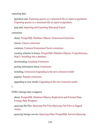
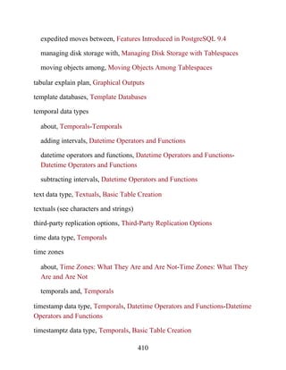
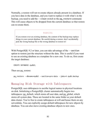
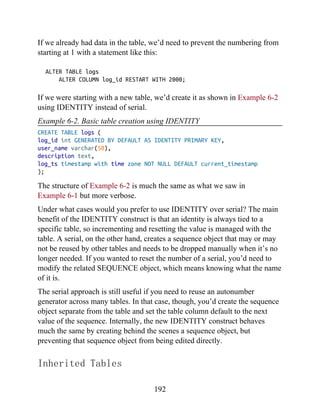
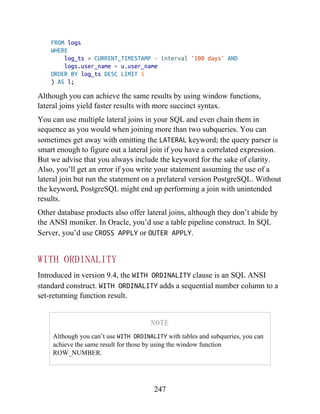
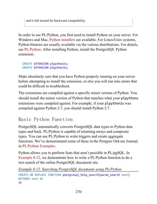
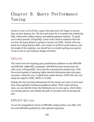
![) As col_name,
fact_type_id
FROM census.lu_fact_types
WHERE category = 'Population' AND fact_subcats[3] ILIKE 'Hispanic or
Latino%'
ORDER BY short_name;
SET @tdef = 'census.hisp_pop(tract_id varchar(11) PRIMARY KEY ';
Loop through records using LINES function.
WHILE @I < LINES(@labels)
BEGIN
SET @tdef = @tdef + ', ' + @labels[@I][0] + ' numeric(12,3) ';
SET @I = @I + 1;
END
SET @tdef = @tdef + ')';
Print out table def.
PRINT @tdef;
create the table.
CREATE TABLE @tdef;
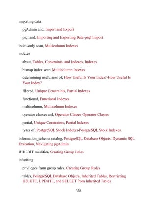
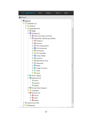
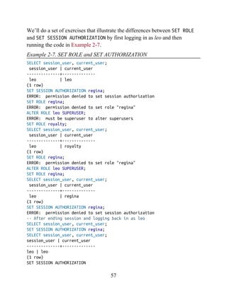
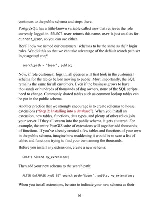
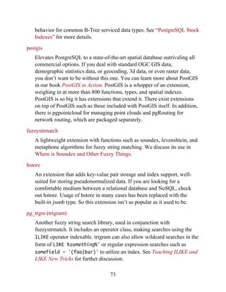
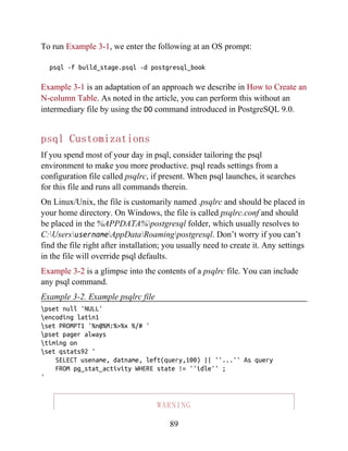
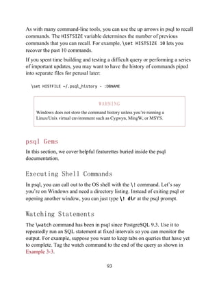
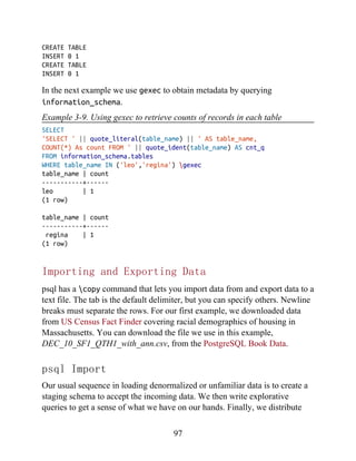
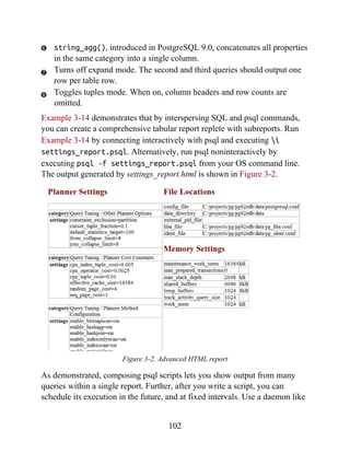
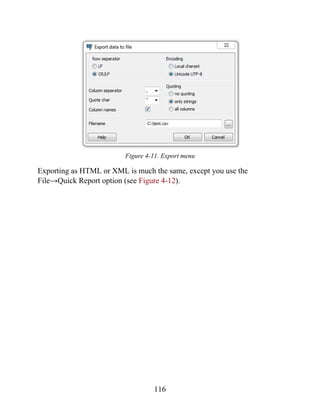
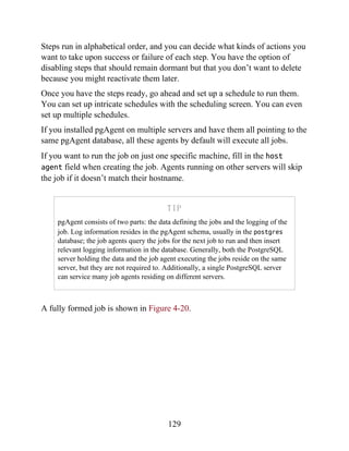
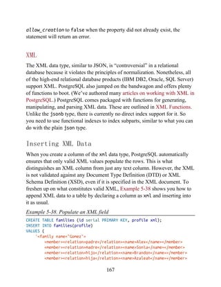
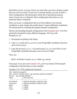
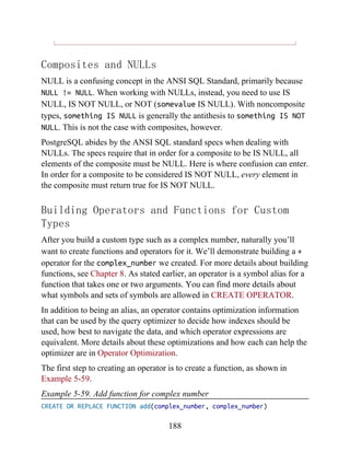
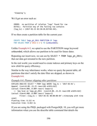
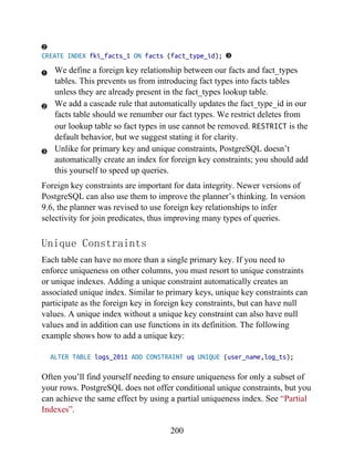
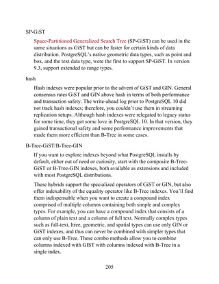
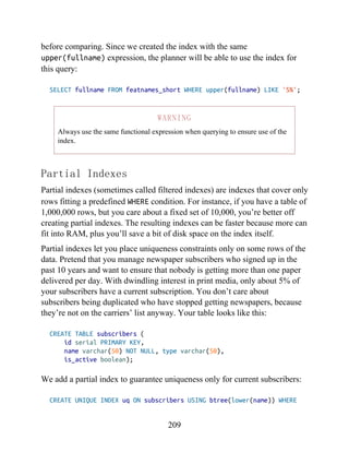
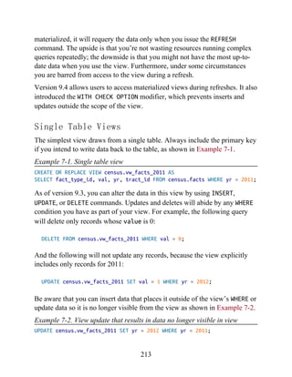
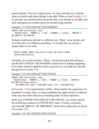
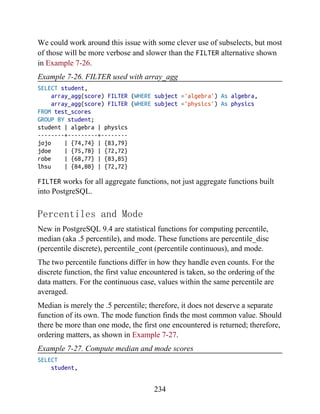
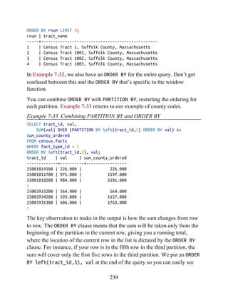
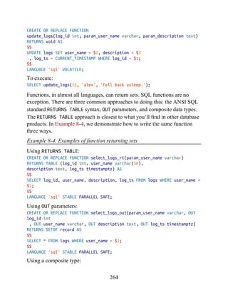
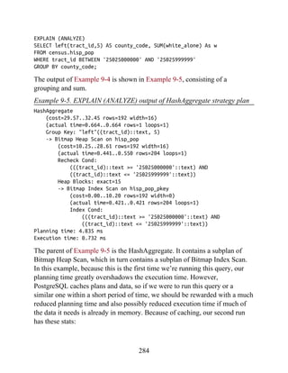
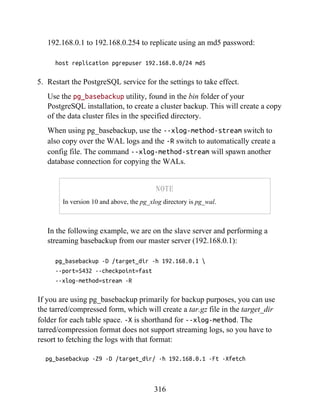
Although pgScript does not have an execute command that allows you to run
dynamically generated SQL, we accomplished the same thing in Example 4-1
by assigning an SQL string to a variable. Example 4-2 pushes the envelope a
bit further by populating the census.hisp_pop table we just created.
Example 4-2. Populating tables with pgScript loop
DECLARE @I, @labels, @tload, @tcols, @fact_types;
SET @I = 0;
SET @labels =
SELECT
quote_ident(
replace(
replace(
lower(COALESCE(fact_subcats[4], fact_subcats[3])), '
', '_'),':'
,''
)
) As col_name,
123](https://image.slidesharecdn.com/postgresqlupandrunningapracticalguidetotheadvancedopensourcedatabasepdfdrive-221213051845-fb16fe5b/85/PostgreSQL_-Up-and-Running_-A-Practical-Guide-to-the-Advanced-Open-Source-Database-PDFDrive-pdf-123-320.jpg)
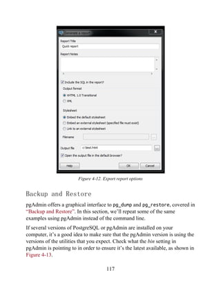
![fact_type_id
FROM census.lu_fact_types
WHERE category = 'Population' AND fact_subcats[3] ILIKE 'Hispanic or
Latino%'
ORDER BY short_name;
SET @tload = 'tract_id';
SET @tcols = 'tract_id';
SET @fact_types = '-1';
WHILE @I < LINES(@labels)
BEGIN
SET @tcols = @tcols + ', ' + @labels[@I][0] ;
SET @tload = @tload +
', MAX(CASE WHEN fact_type_id = ' +
CAST(@labels[@I][1] AS STRING) +
' THEN val ELSE NULL END)';
SET @fact_types = @fact_types + ', ' + CAST(@labels[@I][1] As
STRING);
SET @I = @I + 1;
END
INSERT INTO census.hisp_pop(@tcols)
SELECT @tload FROM census.facts
WHERE fact_type_id IN(@fact_types) AND yr=2010
GROUP BY tract_id;
The lesson to take away from Example 4-2 is that you can dynamically
append SQL fragments into a variable.
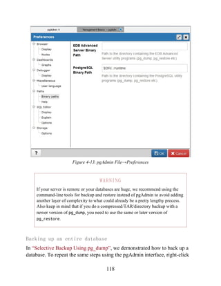
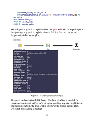
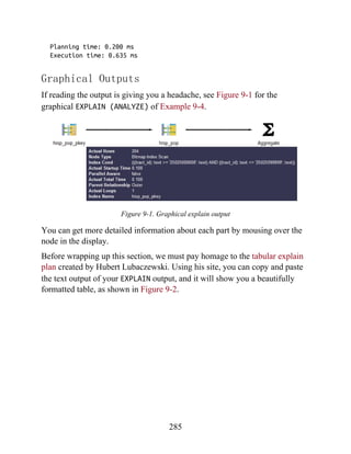
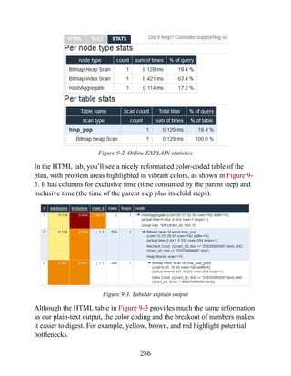
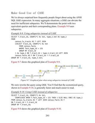
Graphical Explain
One of the great gems in pgAdmin is its at-a-glance graphical explain of the
query plan. You can access the graphical explain plan by opening up an SQL
query window, writing a query, and clicking the explain icon ( ).
Suppose we run the query:
SELECT left(tract_id, 5) As county_code, SUM(hispanic_or_latino) As
tot,
124](https://image.slidesharecdn.com/postgresqlupandrunningapracticalguidetotheadvancedopensourcedatabasepdfdrive-221213051845-fb16fe5b/85/PostgreSQL_-Up-and-Running_-A-Practical-Guide-to-the-Advanced-Open-Source-Database-PDFDrive-pdf-124-320.jpg)
![SELECT unnest(string_to_array('abc.123.z45', '.')) As x;
x
---
abc
123
z45
Regular Expressions and Pattern Matching
PostgreSQL’s regular expression support is downright fantastic. You can
return matches as tables or arrays and choreograph replaces and updates.
Back-referencing and other fairly advanced search patterns are also
supported. In this section, we’ll provide a small sampling. For more
information, see Pattern Matching and String Functions.
Example 5-7 shows you how to format phone numbers stored simply as
contiguous digits.
Example 5-7. Reformat a phone number using back-referencing
SELECT regexp_replace(
'6197306254',
'([0-9]{3})([0-9]{3})([0-9]{4})',
E'(1) 2-3'
) As x;
x
--------------
(619) 730-6254
The 1, 2, etc., refer to elements in our pattern expression. We use a
SELECT split_part('abc.123.z45','.',2) As x;
x
---
123
The string_to_array function is useful for creating an array of elements
from a delimited string. By combining string_to_array with the unnest
function, you can expand the returned array into a set of rows, as shown in
Example 5-6.
Example 5-6. Converting a delimited string to an array to rows
137](https://image.slidesharecdn.com/postgresqlupandrunningapracticalguidetotheadvancedopensourcedatabasepdfdrive-221213051845-fb16fe5b/85/PostgreSQL_-Up-and-Running_-A-Practical-Guide-to-the-Advanced-Open-Source-Database-PDFDrive-pdf-137-320.jpg)
![SELECT unnest(regexp_matches(
'Cell (619) 852-5083. Work (619)123-4567 , Casa 619-730-6254. Bésame
mucho.',
E'[(]{0,1}[0-9]{3}[)-.]{0,1}[s]{0,1}[0-9]{3}[-.]{0,1}[0-9]{4}', 'g')
) As x;
x
--------------
(619) 852-5083
(619)123-4567
619-730-6254
(3 rows)
The matching rules for Example 5-8 are:
[(]{0,1}: starts with zero or one open parenthesis.
[0-9]{3}: followed by three digits.
[)-.]{0,1}: followed by zero or one closed parenthesis, hyphen, or
period.
[s]+: followed by zero or more spaces.
[0-9]{4}: followed by four digits.
regexp_matches returns a string array consisting of matches of a regular
expression. The last input to our function is the flags parameter. We set
this to g, which stands for global and returns all matches of a regular
expression as separate elements. If you leave out this flags parameter,
then your array will only contain the first match. The flags parameter can
consist of more than one flag. For example, if you have letters in your
regular expression and text and you want to make the check case
backslash () to escape the parentheses. The E' construct is PostgreSQL
syntax for denoting that the string to follow should be taken literally.
Suppose some field contains text with embedded phone numbers; Example 5-
8 shows how to extract the phone numbers and turn them into rows all in one
step.
Example 5-8. Return phone numbers in piece of text as separate rows
138](https://image.slidesharecdn.com/postgresqlupandrunningapracticalguidetotheadvancedopensourcedatabasepdfdrive-221213051845-fb16fe5b/85/PostgreSQL_-Up-and-Running_-A-Practical-Guide-to-the-Advanced-Open-Source-Database-PDFDrive-pdf-138-320.jpg)
![insensitive and global, you would use two flags, gi. In addition to the
global flag, other allowed flags are listed in POSIX EMBEDDED
OPTIONS.
unnest explodes an array into a row set.
TIP
There are many ways to compose the same regular expression. For instance,
d is shorthand for [0-9]. But given the few characters you’d save, we prefer
the more descriptive longhand.
If you only care about the first match, you can utilize the substring
function, which will return the first matching value as shown in Example 5-9.
Example 5-9. Return first phone number in piece of text
SELECT substring(
'Cell (619) 852-5083. Work (619)123-4567 , Casa 619-730-6254. Bésame
mucho.'
from E'[(]{0,1}[0-9]{3}[)-.]{0,1}[s]{0,1}[0-9]{3}[-.]{0,1}[0-9]{4}')
As x;
x
----------------
(619) 852-5083
(1 row)
In addition to the wealth of regular expression functions, you can use regular
expressions with the SIMILAR TO (~) operators. The following example
returns all description fields with embedded phone numbers:
SELECT description
FROM mytable
WHERE description ~
E'[(]{0,1}[0-9]{3}[)-.]{0,1}[s]{0,1}[0-9]{3}[-.]{0,1}[0-9]{4}';
Temporals
139](https://image.slidesharecdn.com/postgresqlupandrunningapracticalguidetotheadvancedopensourcedatabasepdfdrive-221213051845-fb16fe5b/85/PostgreSQL_-Up-and-Running_-A-Practical-Guide-to-the-Advanced-Open-Source-Database-PDFDrive-pdf-139-320.jpg)
![generate_series(
'2012-03-11 12:30 AM',
'2012-03-11 3:00 AM',
interval '15 minutes'
) As dt;
dt | hr | mn
-----------------------+----+----------
2012-03-11 00:30:00-05 | 0 | 12:30 AM
2012-03-11 00:45:00-05 | 0 | 12:45 AM
2012-03-11 01:00:00-05 | 1 | 01:00 AM
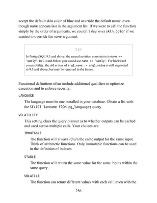
2012-03-11 01:15:00-05 | 1 | 01:15 AM
2012-03-11 01:30:00-05 | 1 | 01:30 AM
2012-03-11 01:45:00-05 | 1 | 01:45 AM
2012-03-11 03:00:00-04 | 3 | 03:00 AM
By default, generate_series assumes timestamptz if you don’t explicitly
cast values to timestamp.
Arrays
Arrays play an important role in PostgreSQL. They are particularly useful in
building aggregate functions, forming IN and ANY clauses, and holding
intermediary values for morphing to other data types. In PostgreSQL, every
data type has a companion array type. If you define your own data type,
PostgreSQL creates a corresponding array type in the background for you.
For example, integer has an integer array type integer[], character has a
character array type character[], and so forth. We’ll show you some useful
functions to construct arrays short of typing them in manually. We will then
point out some handy functions for array manipulations. You can get the
complete listing of array functions and operators in the Official Manual:
Array Functions and Operators.
Array Constructors
The most rudimentary way to create an array is to type the elements:
SELECT ARRAY[2001, 2002, 2003] As yrs;
147](https://image.slidesharecdn.com/postgresqlupandrunningapracticalguidetotheadvancedopensourcedatabasepdfdrive-221213051845-fb16fe5b/85/PostgreSQL_-Up-and-Running_-A-Practical-Guide-to-the-Advanced-Open-Source-Database-PDFDrive-pdf-147-320.jpg)
![If the elements of your array can be extracted from a query, you can use the
more sophisticated constructor function, array():
SELECT array(
SELECT DISTINCT date_part('year', log_ts)
FROM logs
ORDER BY date_part('year', log_ts)
);
Although the array function has to be used with a query returning a single
column, you can specify a composite type as the output, thereby achieving
multicolumn results. We demonstrate this in “Custom and Composite Data
Types”.
You can cast a string representation of an array to an array with syntax of the
form:
SELECT '{Alex,Sonia}'::text[] As name, '{46,43}'::smallint[] As age;
name | age
-------------+--------
{Alex,Sonia} | {46,43}
You can convert delimited strings to an array with the string_to_array
function, as demonstrated in Example 5-15.
Example 5-15. Converting a delimited string to an array
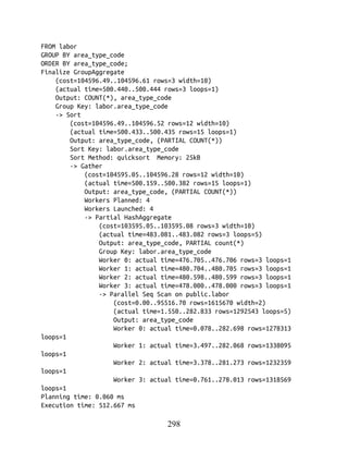
SELECT string_to_array('CA.MA.TX', '.') As estados;
estados
----------
{CA,MA,TX}
(1 row)
array_agg is an aggregate function that can take a set of any data type and
convert it to an array, as demonstrated in Example 5-16.
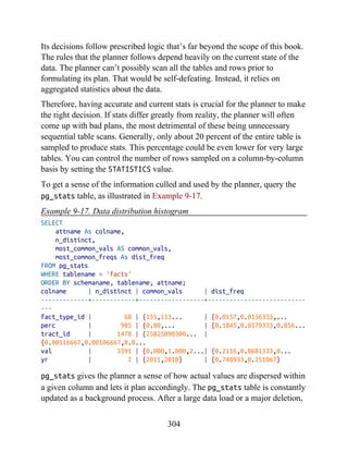
Example 5-16. Using array_agg
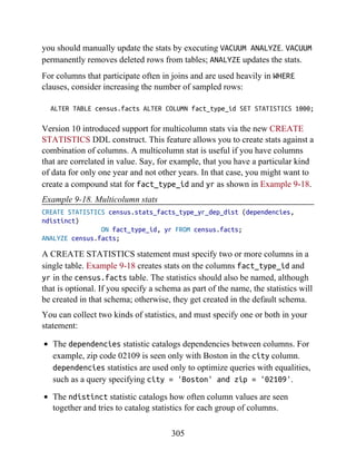
SELECT array_agg(log_ts ORDER BY log_ts) As x
FROM logs
148](https://image.slidesharecdn.com/postgresqlupandrunningapracticalguidetotheadvancedopensourcedatabasepdfdrive-221213051845-fb16fe5b/85/PostgreSQL_-Up-and-Running_-A-Practical-Guide-to-the-Advanced-Open-Source-Database-PDFDrive-pdf-148-320.jpg)
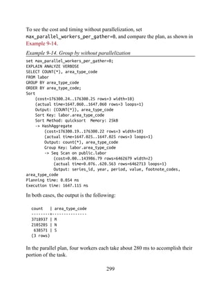
![SELECT array_agg(f.t)
FROM ( VALUES ('{Alex,Sonia}'::text[]),
('{46,43}'::text[] ) ) As f(t);
array_agg
----------------------
{{Alex,Sonia},{46,43}}
(1 row)
In order to aggregate arrays, they must be of the same data type and the same
dimension. To force that in Example 5-17, we cast the ages to text. We also
have the same number of items in the arrays being aggregated: two people
and two ages. Arrays with the same number of elements are called balanced
arrays.
Unnesting Arrays to Rows
A common function used with arrays is unnest, which allows you to expand
the elements of an array into a set of rows, as demonstrated in Example 5-18.
Example 5-18. Expanding arrays with unnest
SELECT unnest('{XOX,OXO,XOX}'::char(3)[]) As tic_tac_toe;
tic_tac_toe
---
XOX
OXO
WHERE log_ts BETWEEN '2011-01-01'::timestamptz AND '2011-01-
15'::timestamptz;
x
------------------------------------------
{'2011-01-01', '2011-01-13', '2011-01-14'}
PostgreSQL 9.5 introduced array_agg function support for arrays. In prior
versions if you wanted to aggregate rows of arrays with array_agg, you’d get
an error. array_agg support for arrays makes it much easier to build
multidimensional arrays from one-dimensional arrays, as shown in
Example 5-17.
Example 5-17. Creating multidimensional arrays from one-dimensional
arrays
149](https://image.slidesharecdn.com/postgresqlupandrunningapracticalguidetotheadvancedopensourcedatabasepdfdrive-221213051845-fb16fe5b/85/PostgreSQL_-Up-and-Running_-A-Practical-Guide-to-the-Advanced-Open-Source-Database-PDFDrive-pdf-149-320.jpg)
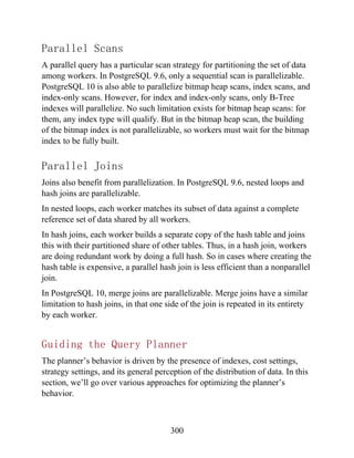
![SELECT
unnest('{three,blind,mice}'::text[]) As t,
unnest('{1,2,3}'::smallint[]) As i;
t |i
------+-
three |1
blind |2
mice |3
If you remove an element of one array so that you don’t have an equal
number of elements in both, you get the result shown in Example 5-20.
Example 5-20. Unnesting unbalanced arrays
SELECT
unnest( '{blind,mouse}'::varchar[]) AS v,
unnest('{1,2,3}'::smallint[]) AS i;
v |i
------+-
blind |1
mouse |2
blind |3
mouse |1
blind |2
mouse |3
Version 9.4 introduced a multiargument unnest function that puts in null
placeholders where the arrays are not balanced. The main drawback with the
new unnest is that it can appear only in the FROM clause. Example 5-21
revisits our unbalanced arrays using the version 9.4 construct.
Example 5-21. Unnesting unbalanced arrays with multiargument unnest
SELECT * FROM unnest('{blind,mouse}'::text[], '{1,2,3}'::int[]) AS
XOX
Although you can add multiple unnests to a single SELECT, if the number of
resultant rows from each array is not balanced, you may get some head-
scratching results.
A balanced unnest, as shown in Example 5-19, yields three rows.
Example 5-19. Unnesting balanced arrays
150](https://image.slidesharecdn.com/postgresqlupandrunningapracticalguidetotheadvancedopensourcedatabasepdfdrive-221213051845-fb16fe5b/85/PostgreSQL_-Up-and-Running_-A-Practical-Guide-to-the-Advanced-Open-Source-Database-PDFDrive-pdf-150-320.jpg)
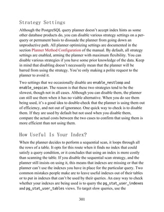
![SELECT fact_subcats[1:2] || fact_subcats[3:4] FROM
census.lu_fact_types;
You can also add additional elements to an existing array as follows:
SELECT '{1,2,3}'::integer[] || 4 || 5;
The result is {1,2,3,4,5}.
Referencing Elements in an Array
Elements in arrays are most commonly referenced using the index of the
element. PostgreSQL array indexes start at 1. If you try to access an element
above the upper bound, you won’t get an error—only NULL will be returned.
The next example grabs the first and last element of our array column:
SELECT
fact_subcats[1] AS primero,
fact_subcats[array_upper(fact_subcats, 1)] As segundo
FROM census.lu_fact_types;
f(t,i);
t | i
-------+---
blind | 1
mouse | 2
<NULL> | 3
Array Slicing and Splicing
PostgreSQL also supports array slicing using the start:end syntax. It
returns another array that is a subarray of the original. For example, to return
new arrays that just contain elements 2 through 4 of each original array, type:
SELECT fact_subcats[2:4] FROM census.lu_fact_types;
To glue two arrays together end to end, use the concatenation operator ||:
151](https://image.slidesharecdn.com/postgresqlupandrunningapracticalguidetotheadvancedopensourcedatabasepdfdrive-221213051845-fb16fe5b/85/PostgreSQL_-Up-and-Running_-A-Practical-Guide-to-the-Advanced-Open-Source-Database-PDFDrive-pdf-151-320.jpg)
![SELECT fact_subcats
FROM census.lu_fact_types
WHERE fact_subcats && '{OCCUPANCY STATUS,For rent}'::varchar[];
fact_subcats
-----------------------------------------------------------
{S01,"OCCUPANCY STATUS","Total housing units"...}
{S02,"OCCUPANCY STATUS","Total housing units"...}
{S03,"OCCUPANCY STATUS","Total housing units"...}
{S10,"VACANCY STATUS","Vacant housing units","For rent"...}
(4 rows)
The equality operator (=) returns true only if elements in all the arrays are
equal and in the same order. If you don’t care about order of elements, and
just need to know whether all the elements in one array appear as a subset of
the other array, use the containment operators (@> , <@). Example 5-23
demonstrates the difference between the contains (@>) and contained by (@<)
operators.
We used the array_upper function to get the upper bound of the array. The
second required parameter of the function indicates the dimension. In our
case, our array is one-dimensional, but PostgreSQL does support
multidimensional arrays.
Array Containment Checks
PostgreSQL has several operators for working with array data. We already
saw the concatenation operator (||) for combining multiple arrays into one or
adding an element to an array in “Array Slicing and Splicing”. Arrays also
support the following comparison operators: =, <>, <, >, @>, <@, and &&. These
operators require both sides of the operator to be arrays of the same array data
type. If you have a GiST or GIN index on your array column, the comparison
operators can utilize them.
The overlap operator (&&) returns true if two arrays have any elements in
common. Example 5-22 will list all records in our table where the
fact_subcats contains elements OCCUPANCY STATUS or For rent.
Example 5-22. Array overlaps operator
152](https://image.slidesharecdn.com/postgresqlupandrunningapracticalguidetotheadvancedopensourcedatabasepdfdrive-221213051845-fb16fe5b/85/PostgreSQL_-Up-and-Running_-A-Practical-Guide-to-the-Advanced-Open-Source-Database-PDFDrive-pdf-152-320.jpg)
![Example 5-23. Array containment operators
SELECT '{1,2,3}'::int[] @> '{3,2}'::int[] AS contains;
contains
--------
t
(1 row)
SELECT '{1,2,3}'::int[] <@ '{3,2}'::int[] AS contained_by;
contained_by
------------
f
(1 row)
Range Types
Range data types represent data with a beginning and an end. PostgreSQL
also rolled out many operators and functions to identify overlapping ranges,
check to see whether a value falls inside the range, and combine adjacent
smaller ranges into larger ranges. Prior to range types, we had to kludge our
own functions. These often were clumsy and slow, and didn’t always produce
the expected results. We’ve been so happy with ranges that we’ve converted
all of our temporal tables to use them where possible. We hope you share our
joy.
Range types replace the need to use two separate fields to represent ranges.
Suppose we want all integers between −2 and 2, but not including 2. The
range representation would be [-2,2). The square bracket indicates a range
that is closed on that end, whereas a parenthesis indicates a range that is open
on that end. Thus, [-2,2) includes exactly four integers: −2, −1, 0, 1.
Similarly:
The range (-2,2] includes four integers: -1, 0, 1, 2.
The range (-2,2) includes three integers: -1, 0, 1.
The range [-2,2] includes five integers: -2, -1, 0, 1, 2.
Discrete Versus Continuous Ranges
153](https://image.slidesharecdn.com/postgresqlupandrunningapracticalguidetotheadvancedopensourcedatabasepdfdrive-221213051845-fb16fe5b/85/PostgreSQL_-Up-and-Running_-A-Practical-Guide-to-the-Advanced-Open-Source-Database-PDFDrive-pdf-153-320.jpg)
![A range of integers. Integer ranges are discrete and subject to
canonicalization.
numrange
A continuous range of decimals, floating-point numbers, or double-
precision numbers.
daterange
A discrete date range of calendar dates without time zone awareness.
tsrange, tstzrange
A continuous date and time (timestamp) range allowing for fractional
seconds. tstrange is not time zone−aware; tstzrange is time zone
PostgreSQL makes a distinction between discrete and continuous ranges. A
range of integers or dates is discrete because you can enumerate each value
within the range. Think of dots on a number line. A range of numerics or
timestamps is continuous, because an infinite number of values lies between
the end points.
A discrete range has multiple representations. Our earlier example of [-2,2)
can be represented in the following ways and still include the same number of
values in the range: [-2,1], (-3,1], (-3,2), [-2,2). Of these four
representations, the one with [) is considered the canonical form. There’s
nothing magical about closed-open ranges except that if everyone agrees to
using that representation for discrete ranges, we can easily compare among
many ranges without having to worry first about converting open to close or
vice versa. PostgreSQL canonicalizes all discrete ranges, for both storage and
display. So if you enter a date range as (2014-1-5,2014-2-1], PostgreSQL
rewrites it as [2014-01-06,2014-02-02).
Built-in Range Types
PostgreSQL comes with six built-in range types for numbers and datetimes:
int4range, int8range
154](https://image.slidesharecdn.com/postgresqlupandrunningapracticalguidetotheadvancedopensourcedatabasepdfdrive-221213051845-fb16fe5b/85/PostgreSQL_-Up-and-Running_-A-Practical-Guide-to-the-Advanced-Open-Source-Database-PDFDrive-pdf-154-320.jpg)
![SELECT '[2013-01-05,2013-08-13]'::daterange;
SELECT '(2013-01-05,2013-08-13]'::daterange;
SELECT '(0,)'::int8range;
SELECT '(2013-01-05 10:00,2013-08-13 14:00]'::tsrange;
[2013-01-05,2013-08-14)
[2013-01-06,2013-08-14)
[1,)
("2013-01-05 10:00:00","2013-08-13 14:00:00"]
A date range between 2013-01-05 and 2013-08-13 inclusive. Note the
canonicalization on the upper bound.
A date range greater than 2013-01-05 and less than or equal to 2013-08-
13. Notice the canonicalization.
All integers greater than 0. Note the canonicalization.
A timestamp greater than 2013-01-05 10:00 AM and less than or equal to
2013-08-13 2 PM.
−aware.
For number-like ranges, if either the start point or the end point is left blank,
PostgreSQL replaces it with a null. For practicality, you can interpret the null
to represent either -infinity on the left or infinity on the right. In
actuality, you’re bound by the smallest and largest values for the particular
data type. So a int4range of (,) would be [-2147483648,2147483647).
For temporal ranges, -infinity and infinity are valid upper and lower
bounds.
In addition to the built-in range types, you can create your own range types.
When you do, you can set the range to be either discrete or continuous.
Defining Ranges
A range, regardless of type, is always comprised of two elements of the same
type with the bounding condition denoted by brackets or parentheses, as
shown in Example 5-24.
Example 5-24. Defining ranges with casts
155](https://image.slidesharecdn.com/postgresqlupandrunningapracticalguidetotheadvancedopensourcedatabasepdfdrive-221213051845-fb16fe5b/85/PostgreSQL_-Up-and-Running_-A-Practical-Guide-to-the-Advanced-Open-Source-Database-PDFDrive-pdf-155-320.jpg)
![TIP
Datetimes in PostgreSQL can take on the values of -infinity and infinity.
For uniformity and in keeping with convention, we suggest that you always use
[ for the former and ) for the latter as in [-infinity, infinity).
Ranges can also be defined using range constructor functions, which go by
the same name as the range and can take two or three arguments. Here’s an
example:
SELECT daterange('2013-01-05','infinity','[]');
The third argument denotes the bound. If omitted, the open-close [)
convention is used by default. We suggest that you always include the third
element for clarity.
Defining Tables with Ranges
Temporal ranges are popular. Suppose you have an employment table that
stores employment history. Instead of creating separate columns for start and
end dates, you can design a table as shown in Example 5-25. In the example,
we added an index to the period column to speed up queries using our range
column.
Example 5-25. Table with date range
CREATE TABLE employment (id serial PRIMARY KEY, employee varchar(20),
period daterange);
CREATE INDEX ix_employment_period ON employment USING gist (period);
INSERT INTO employment (employee,period)
VALUES
('Alex','[2012-04-24, infinity)'::daterange),
('Sonia','[2011-04-24, 2012-06-01)'::daterange),
('Leo','[2012-06-20, 2013-04-20)'::daterange),
('Regina','[2012-06-20, 2013-04-20)'::daterange);
Add a GiST index on the range field.
156](https://image.slidesharecdn.com/postgresqlupandrunningapracticalguidetotheadvancedopensourcedatabasepdfdrive-221213051845-fb16fe5b/85/PostgreSQL_-Up-and-Running_-A-Practical-Guide-to-the-Advanced-Open-Source-Database-PDFDrive-pdf-156-320.jpg)
![{
"father":"Rafael",
"mother":"Ofelia"
},
"phones":
[
{
"type":"work",
"number":"619-722-6719"
},
{
"type":"cell",
"number":"619-852-5083"
}
]
},
"children":
[
{
"name":"Brandon",
"gender":"M"
},
{
"name":"Azaleah",
"girl":true,
"phones": []
}
]
}'
);
Querying JSON
The easiest way to traverse the hierarchy of a JSON object is by using pointer
symbols. Example 5-29 shows some common usage.
Example 5-29. Querying the JSON field
SELECT person->'name' FROM persons;
SELECT person->'spouse'->'parents'->'father' FROM persons;
You can also write the query using a path array as in the following example:
159](https://image.slidesharecdn.com/postgresqlupandrunningapracticalguidetotheadvancedopensourcedatabasepdfdrive-221213051845-fb16fe5b/85/PostgreSQL_-Up-and-Running_-A-Practical-Guide-to-the-Advanced-Open-Source-Database-PDFDrive-pdf-159-320.jpg)
![SELECT person#>array['spouse','parents','father'] FROM persons;
Notice that you must use the #> pointer symbol if what comes after is a path
array.
To penetrate JSON arrays, specify the array index. JSON arrays is zero-
indexed, unlike PostgreSQL arrays, whose indexes start at 1.
SELECT person->'children'->0->'name' FROM persons;
And the path array equivalent:
SELECT person#>array['children','0','name'] FROM persons;
All queries in the prior examples return the value as JSON primitives
(numbers, strings, booleans). To return the text representation, add another
greater-than sign as in the following examples:
SELECT person->'spouse'->'parents'->>'father' FROM persons;
SELECT person#>>array['children','0','name'] FROM persons;
If you are chaining the -> operator, only the very last one can be a ->>
operator.
The json_array_elements function takes a JSON array and returns each
element of the array as a separate row as in Example 5-30.
Example 5-30. json_array_elements to expand JSON array
SELECT json_array_elements(person->'children')->>'name' As name FROM
persons;
name
-------
Brandon
Azaleah
(2 rows)
NOTE
160](https://image.slidesharecdn.com/postgresqlupandrunningapracticalguidetotheadvancedopensourcedatabasepdfdrive-221213051845-fb16fe5b/85/PostgreSQL_-Up-and-Running_-A-Practical-Guide-to-the-Advanced-Open-Source-Database-PDFDrive-pdf-160-320.jpg)
![converts it to a canonical text representation, as shown in Example 5-32.
Example 5-32. jsonb versus json output
SELECT person As b FROM persons_b WHERE id = 1;
SELECT person As j FROM persons WHERE id = 1;
b
-------------------------------------------------------------------------
--------
{"name": "Sonia",
"spouse": {"name": "Alex", "phones": [{"type": "work", "number": "619-
722-6719"},
{"type": "cell", "number": "619-852-5083"}],
"parents": {"father": "Rafael", "mother": "Ofelia"}},
"children": [{"name": "Brandon", "gender": "M"},
{"girl": true, "name": "Azaleah", "phones": []}]}
(1 row)
j
---------------------------------------------
{
"name":"Sonia",
"spouse":
{
"name":"Alex",
"parents":
{
"father":"Rafael",
"mother":"Ofelia"
},
"phones":
[
{
"type":"work",
"number":"619-722-6719"+
},
{
"type":"cell",
"number":"619-852-5083"+
}
]
},
"children":
[
163](https://image.slidesharecdn.com/postgresqlupandrunningapracticalguidetotheadvancedopensourcedatabasepdfdrive-221213051845-fb16fe5b/85/PostgreSQL_-Up-and-Running_-A-Practical-Guide-to-the-Advanced-Open-Source-Database-PDFDrive-pdf-163-320.jpg)
![{
"name":"Brandon",
"gender":"M"
},
{
"name":"Azaleah",
"girl":true,
"phones": []
}
]
}
(1 row)
jsonb reformats input and removes whitespace. Also, the order of
attributes is not maintained from the insert.
json maintains input whitespace and the order of attributes.
jsonb has similarly named functions as json, plus some additional ones. So,
for example, the json family of functions such as json_extract_path_text
and json_each are matched in jsonb by jsonb_extract_path_text,
jsonb_each, etc. However, the equivalent operators are the same, so you will
find that the examples in “Querying JSON” work largely the same without
change for the jsonb type—just replace the table name and
json_array_elements with jsonb_array_elements.
In addition to the operators supported by json, jsonb has additional
comparator operators for equality (=), contains (@>), contained (<@), key
exists (?), any of array of keys exists (?|), and all of array of keys exists (?&).
So, for example, to list all people that have a child named Brandon, use the
contains operator as demonstrated in Example 5-33.
Example 5-33. jsonb contains operator
SELECT person->>'name' As name
FROM persons_b
WHERE person @> '{"children":[{"name":"Brandon"}]}';
name
-----
Sonia
164](https://image.slidesharecdn.com/postgresqlupandrunningapracticalguidetotheadvancedopensourcedatabasepdfdrive-221213051845-fb16fe5b/85/PostgreSQL_-Up-and-Running_-A-Practical-Guide-to-the-Advanced-Open-Source-Database-PDFDrive-pdf-164-320.jpg)
![UPDATE persons_b
SET person = person - 'address'
WHERE person @> '{"name":"Sonia"}';
The simple - operator works for first-level elements, but what if you wanted
to remove an attribute from a particular member? This is when you’d use the
#- operator. #- takes an array of text values that denotes the path of the
element you want to remove. In Example 5-36 we remove the girl
designator of Azaleah.
Example 5-36. Using JSONB #- to remove nested element
UPDATE persons_b
SET person = person #- '{children,1,girl}'::text[]
WHERE person @> '{"name":"Sonia"}'
RETURNING person->'children'->1;
{"name": "Azaleah", "phones": []}
When removing elements from an array, you need to denote the index.
Because JavaScript indexes start at 0, to remove an element from the second
child, we use 1 instead of 2. If we wanted to remove Azaleah entirely, we
would have used '{children,1}'::text[].
To add a gender attribute, or replace one that was previously set, we can use
the jsonb_set function as shown in Example 5-37.
Example 5-37. Using the jsonb_set function to change a nested value
UPDATE persons_b
SET person = jsonb_set(person,'{children,1,gender}'::text[],'"F"'::jsonb,
true)
WHERE person @> '{"name":"Sonia"}';
jsonb_set takes three arguments of form jsonb_set(jsonb_to_update,
text_array_path, new_jsonb_value,allow_creation). If you set
Somewhere in San Diego, CA with something else.
If we decided we no longer wanted an address, we could use the - as shown
in Example 5-35.
Example 5-35. Using JSONB - to remove an element
166](https://image.slidesharecdn.com/postgresqlupandrunningapracticalguidetotheadvancedopensourcedatabasepdfdrive-221213051845-fb16fe5b/85/PostgreSQL_-Up-and-Running_-A-Practical-Guide-to-the-Advanced-Open-Source-Database-PDFDrive-pdf-166-320.jpg)
![</family>');
Each XML value could have a different XML structure. To enforce
uniformity, you can add a check constraint, covered in “Check Constraints”,
to the XML column. Example 5-39 ensures that all family has at least one
relation element. The '/family/member/relation' is XPath syntax, a
basic way to refer to elements and other parts of XML.
Example 5-39. Ensure that all records have at least one member relation
ALTER TABLE families ADD CONSTRAINT chk_has_relation
CHECK (xpath_exists('/family/member/relation', profile));
If we then try to insert something like:
INSERT INTO families (profile) VALUES ('<family name="HsuObe">
</family>');
we will get this error: ERROR: new row for relation "families"
violates check constraint "chk_has_relation".
For more involved checks that require checking against DTD or XSD, you’ll
need to resort to writing functions and using those in the check constraint,
because PostgreSQL doesn’t have built-in functions to handle those kinds of
checks.
Querying XML Data
To query XML, the xpath function is really useful. The first argument is an
XPath query, and the second is an xml object. The output is an array of XML
elements that satisfies the XPath query. Example 5-40 combines xpath with
unnest to return all the family members. unnest unravels the array into a
row set. We then cast the XML fragment to text.
Example 5-40. Query XML field
SELECT ordinality AS id, family,
(xpath('/member/relation/text()', f))[1]::text As relation,
(xpath('/member/name/text()', f))[1]::text As mem_name
FROM (
168](https://image.slidesharecdn.com/postgresqlupandrunningapracticalguidetotheadvancedopensourcedatabasepdfdrive-221213051845-fb16fe5b/85/PostgreSQL_-Up-and-Running_-A-Practical-Guide-to-the-Advanced-Open-Source-Database-PDFDrive-pdf-168-320.jpg)
![SELECT
(xpath('/family/@name', profile))[1]::text As family,
f.ordinality, f.f
FROM families, unnest(xpath('/family/member', profile)) WITH
ORDINALITY AS f
) x;
id | family | relation | mem_name
----+--------+----------+----------
1 | Gomez | padre | Alex
2 | Gomez | madre | Sonia
3 | Gomez | hijo | Brandon
4 | Gomez | hija | Azaleah
(4 rows)
Get the text element in the relation and name tags of each member
element. We need to use array subscripting because xpath always returns
an array, even if only one element is returned.
Get the name attribute from family root. For this we use
@attribute_name.
Break the result of the SELECT into the subelements <member>,
<relation>, </relation>, <name>, </name>, and </member> tags. The
slash is a way of getting at subtag elements. For example,
xpath('/family/member', 'profile') will return an array of all
members in each family that is defined in a profile. The @ sign is used to
select attributes of an element. So, for example, family/@name returns
the name attribute of a family. By default, xpath always returns an
element, including the tag part. The text() forces a return of just the text
body of an element.
New in version 10 is the ANSI-SQL standard XMLTABLE construct.
XMLTABLE converts text of XML into individual rows and columns based
on some defined transformation. We’ll repeat Example 5-40 using
XMLTABLE.
Example 5-41. Query XML using XMLTABLE
SELECT xt.*
FROM families,
XMLTABLE ('/family/member' PASSING profile
169](https://image.slidesharecdn.com/postgresqlupandrunningapracticalguidetotheadvancedopensourcedatabasepdfdrive-221213051845-fb16fe5b/85/PostgreSQL_-Up-and-Running_-A-Practical-Guide-to-the-Advanced-Open-Source-Database-PDFDrive-pdf-169-320.jpg)
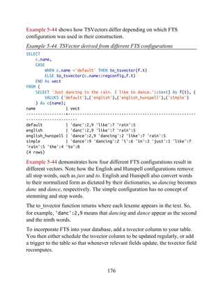
![Example 5-54. Ranking search results using custom weights
SELECT
left(title,40) As title,
ts_rank('{0,0,0,1}'::numeric[],fts,ts)::numeric(10,3) AS r,
ts_rank_cd('{0,0,0,1}'::numeric[],fts,ts)::numeric(10,3) As rcd
FROM film, to_tsquery('english', 'love & (wait | indian | mad )') AS ts
WHERE fts @@ ts AND title > ''
ORDER BY r DESC;
title | r | rcd
--------------+-------+------
INDIAN LOVE | 0.991 | 1.000
LAWRENCE LOVE | 0.000 | 0.000
(2 rows)
Notice how in Example 5-54 the second entry has a ranking of zero because
the title does not contain all the words to satisfy the tsquery.
NOTE
If performance is a concern, you should explicitly declare the FTS
configuration in queries instead of allowing the default behavior. As noted in
Some FTS Tricks by Oleg Bartunov, you can achieve twice the speed by using
to_tsquery('english','social & (science | scientist)') in lieu of
to_tsquery('social & (science | scientist)').
Full Text Stripping
By default, vectorization adds markers (location of the lexemes within the
vector) and optionally weights (A, B, C, D). If your searches care only
whether a particular term can be found, regardless of where it is in the text,
how frequently it occurs, or its prominence, you can declutter your vectors
using the strip function. This saves disk space and gains some speed.
Example 5-55 compares what an unstripped versus stripped vector looks like.
Example 5-55. Unstripped versus stripped vector
SELECT fts
FROM film
183](https://image.slidesharecdn.com/postgresqlupandrunningapracticalguidetotheadvancedopensourcedatabasepdfdrive-221213051845-fb16fe5b/85/PostgreSQL_-Up-and-Running_-A-Practical-Guide-to-the-Advanced-Open-Source-Database-PDFDrive-pdf-183-320.jpg)
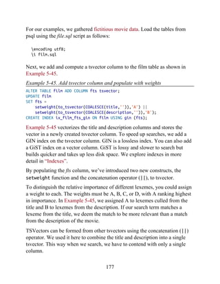
![SELECT ts_headline(person->'spouse'->'parents', 'rafael'::tsquery)
FROM persons_b WHERE id=1;
{"father": "<b>Rafael</b>", "mother": "Ofelia"}
(1 row)
Note the bold HTML tags around the matching value.
Custom and Composite Data Types
This section demonstrates how to define and use a custom type. The
composite (aka record, row) object type is often used to build an object that
is then cast to a custom type, or as a return type for functions needing to
return multiple columns.
All Tables Are Custom Data Types
PostgreSQL automatically creates custom types for all tables. For all intents
and purposes, you can use custom types just as you would any other built-in
type. So we could conceivably create a table that has a column type that is
another table’s custom type, and we can go even further and make an array of
that type. We demonstrate this “turducken” in Example 5-58.
Example 5-58. Turducken
CREATE TABLE chickens (id integer PRIMARY KEY);
CREATE TABLE ducks (id integer PRIMARY KEY, chickens chickens[]);
CREATE TABLE turkeys (id integer PRIMARY KEY, ducks ducks[]);
INSERT INTO ducks VALUES (1, ARRAY[ROW(1)::chickens, ROW(1)::chickens]);
INSERT INTO turkeys VALUES (1, array(SELECT d FROM ducks d));
We create an instance of a chicken without adding it to the chicken table
and populate the field using either a trigger or update as needed.
Also available now for json and jsonb is the ts_headline function, which
tags as HTML all matching text in the json document. Example 5-57 flags all
references to Rafael in the document.
Example 5-57. Tag matching words
185](https://image.slidesharecdn.com/postgresqlupandrunningapracticalguidetotheadvancedopensourcedatabasepdfdrive-221213051845-fb16fe5b/85/PostgreSQL_-Up-and-Running_-A-Practical-Guide-to-the-Advanced-Open-Source-Database-PDFDrive-pdf-185-320.jpg)
![SELECT * FROM turkeys;
output
--------------------------
id | ducks
---+----------------------
1 | {"(1,"{(1),(1)}")"}
We can also replace subelements of our turducken. This next example
replaces our second chicken in our first turkey with a different chicken:
UPDATE turkeys SET ducks[1].chickens[2] = ROW(3)::chickens
WHERE id = 1 RETURNING *;
output
--------------------------
id | ducks
---+----------------------
1 | {"(1,"{(1),(3)}")"}
We used the RETURNING clause as discussed in “Returning Affected Records
to the User” to output the changed record.
Any complex row or column, regardless of how complex, can be converted to
a json or jsonb column like so:
SELECT id, to_jsonb(ducks) AS ducks_jsonb
FROM turkeys;
id | ducks_jsonb
---+------------------------------------------------
1 | [{"id": 1, "chickens": [{"id": 1}, {"id": 3}]}]
(1 row)
itself; hence we’re able to repeat id with impunity. We take our array of two
chickens, stuff them into one duck, and add it to the ducks table. We take the
duck we added and stuff it into the turkeys table.
Finally, let’s see what we have in our turkey:
186](https://image.slidesharecdn.com/postgresqlupandrunningapracticalguidetotheadvancedopensourcedatabasepdfdrive-221213051845-fb16fe5b/85/PostgreSQL_-Up-and-Running_-A-Practical-Guide-to-the-Advanced-Open-Source-Database-PDFDrive-pdf-186-320.jpg)
![the usual equality operator for the room number.
Example 6-10. Prevent overlapping bookings for the same room
CREATE TABLE schedules(id serial primary key, room int, time_slot
tstzrange);
ALTER TABLE schedules ADD CONSTRAINT ex_schedules
EXCLUDE USING gist (room WITH =, time_slot WITH &&);
Just as with uniqueness constraints, PostgreSQL automatically creates a
corresponding index of the type specified in the constraint declaration.
Arrays are another popular type where EXCLUSION constraints come in
handy. Let’s suppose you have a set of rooms that you need to assign to a
group of people. We’ll call these room “blocks.” For expediency, you decide
to store one record per party, but you want to ensure that two parties are
never given the same room. So you set up a table as follows:
CREATE TABLE room_blocks(block_id integer primary key, rooms int[]);
To ensure that no two blocks have a room in common, you can set up an
exclusion constraint preventing blocks from overlapping (two blocks having
the same room). Exclusion constraints unfortunately work only with GiST
indexes, and because GIST indexes don’t exist for arrays out of the box, you
need to install an additional extension before you can do this, as shown in
Example 6-11.
Example 6-11. Prevent overlapping array blocks
CREATE EXTENSION IF NOT EXISTS intarray;
ALTER TABLE room_blocks
ADD CONSTRAINT ex_room_blocks_rooms
EXCLUDE USING gist(rooms WITH &&);
The intarray extension provides GiST index support for integer arrays (int4,
int8). After intarray is installed, you can then use GiST with arrays and create
exclusion constraints on integer arrays.
Indexes
202](https://image.slidesharecdn.com/postgresqlupandrunningapracticalguidetotheadvancedopensourcedatabasepdfdrive-221213051845-fb16fe5b/85/PostgreSQL_-Up-and-Running_-A-Practical-Guide-to-the-Advanced-Open-Source-Database-PDFDrive-pdf-202-320.jpg)
![SELECT tract_name FROM census.lu_tracts WHERE tract_name ILIKE
'%duke%';
tract_name
------------------------------------------------
Census Tract 2001, Dukes County, Massachusetts
Census Tract 2002, Dukes County, Massachusetts
Census Tract 2003, Dukes County, Massachusetts
Census Tract 2004, Dukes County, Massachusetts
Census Tract 9900, Dukes County, Massachusetts
ANY Array Search
PostgreSQL has a construct called ANY that can be used in conjunction with
arrays, combined with a comparator operator or comparator keyword. If any
element of the array matches a row, that row is returned.
Here is an example:
SELECT tract_name
FROM census.lu_tracts
WHERE tract_name ILIKE
ANY(ARRAY['%99%duke%','%06%Barnstable%']::text[]);
tract_name
-----------------------------------------------------
Census Tract 102.06, Barnstable County, Massachusetts
Census Tract 103.06, Barnstable County, Massachusetts
Census Tract 106, Barnstable County, Massachusetts
Census Tract 9900, Dukes County, Massachusetts
(4 rows)
The example just shown is a shorthand way of using multiple ILIKE OR
clauses. You can use ANY with other comparators such as LIKE, =, and ~ (the
regex like operator).
ANY can be used with any data types and comparison operators (operators that
return a Boolean), including ones you built yourself or installed via
extensions.
223](https://image.slidesharecdn.com/postgresqlupandrunningapracticalguidetotheadvancedopensourcedatabasepdfdrive-221213051845-fb16fe5b/85/PostgreSQL_-Up-and-Running_-A-Practical-Guide-to-the-Advanced-Open-Source-Database-PDFDrive-pdf-223-320.jpg)
![UPDATE census.lu_fact_types AS f
SET short_name = replace(replace(lower(f.fact_subcats[4]),'
','_'),':','')
WHERE f.fact_subcats[3] = 'Hispanic or Latino:' AND f.fact_subcats[4] >
''
RETURNING fact_type_id, short_name;
fact_type_id | short_name
-------------+-------------------------------------------------
96 | white_alone
97 | black_or_african_american_alone
98 | american_indian_and_alaska_native_alone
99 | asian_alone
100 | native_hawaiian_and_other_pacific_islander_alone
101 | some_other_race_alone
102 | two_or_more_races
UPSERTs: INSERT ON CONFLICT UPDATE
New in version 9.5 is the INSERT ON CONFLICT construct, which is often
referred to as an UPSERT. This feature is useful if you don’t know a record
already exists in a table and rather than having the insert fail, you want it to
either update the existing record or do nothing.
This feature requires a unique key, primary key, unique index, or exclusion
constraint in place, that when violated, you’d want different behavior like
updating the existing record or not doing anything. To demonstrate, imagine
we have a table of colors to create:
CREATE TABLE colors(color varchar(50) PRIMARY KEY, hex varchar(6));
INSERT INTO colors(color, hex)
VALUES('blue', '0000FF'), ('red', 'FF0000');
We then get a new batch of colors to add to our table, but some may be
RETURNING is invaluable because it returns the key value of the new rows—
something you wouldn’t know prior to the query execution. Although
RETURNING is often accompanied by * for all fields, you can limit the fields as
we do in Example 7-16.
Example 7-16. Returning changed records of an UPDATE with RETURNING
226](https://image.slidesharecdn.com/postgresqlupandrunningapracticalguidetotheadvancedopensourcedatabasepdfdrive-221213051845-fb16fe5b/85/PostgreSQL_-Up-and-Running_-A-Practical-Guide-to-the-Advanced-Open-Source-Database-PDFDrive-pdf-226-320.jpg)
![SELECT array_to_json(array_agg(f)) As cat
FROM (
SELECT MAX(fact_type_id) As max_type, category
FROM census.lu_fact_types
GROUP BY category
) As f;
This will give you an output of:
cats
----------------------------------------------------
[{"max_type":102,"category":"Population"},
{"max_type":153,"category":"Housing"}]
Defines a subquery with name f. f can then be used to reference each row
in the subquery.
Aggregate each row of subquerying using array_agg and then convert the
array to json with array_to_json.
In version 9.3, the json_agg function replaces the chain of array_to_json
and array_agg, offering both convenience and speed. In Example 7-21, we
repeat Example 7-20 using json_agg, and both examples will have the same
output.
Example 7-21. Query to JSON using json_agg
SELECT json_agg(f) As cats
FROM (
SELECT MAX(fact_type_id) As max_type, category
FROM census.lu_fact_types
GROUP BY category
) As f;
Dollar Quoting
In standard ANSI SQL, single quotes (') surround string literals. Should you
array_agg and array_to_json to output a query as a single JSON object as
shown in Example 7-20. In PostgreSQL 9.4, you can use json_agg. See
Example 7-21.
Example 7-20. Query to JSON output
229](https://image.slidesharecdn.com/postgresqlupandrunningapracticalguidetotheadvancedopensourcedatabasepdfdrive-221213051845-fb16fe5b/85/PostgreSQL_-Up-and-Running_-A-Practical-Guide-to-the-Advanced-Open-Source-Database-PDFDrive-pdf-229-320.jpg)
![set search_path=census;
DROP TABLE IF EXISTS lu_fact_types CASCADE;
CREATE TABLE lu_fact_types (
fact_type_id serial,
category varchar(100),
fact_subcats varchar(255)[],
short_name varchar(50),
CONSTRAINT pk_lu_fact_types PRIMARY KEY (fact_type_id)
);
Then we’ll use DO to populate it as shown in Example 7-22. CASCADE will
force the drop of any related objects such as foreign key constraints and
views, so be cautious when using CASCADE.
Example 7-22 generates a series of INSERT INTO SELECT statements. The
SQL also performs an unpivot operation to convert columnar data into rows.
WARNING
Example 7-22 is only a partial listing of the code needed to build
lu_fact_types. For the full code, refer to the building_census_tables.sql file
that is part of the book code and data download.
Example 7-22. Using DO to generate dynamic SQL
DO language plpgsql
$$
DECLARE var_sql text;
BEGIN
var_sql := string_agg(
$sql$
INSERT INTO lu_fact_types(category, fact_subcats, short_name)
SELECT
'Housing',
from our staging table. We’ll use PL/pgSQL for our procedural snippet, but
you’re free to use other languages.
First, we’ll create the table:
231](https://image.slidesharecdn.com/postgresqlupandrunningapracticalguidetotheadvancedopensourcedatabasepdfdrive-221213051845-fb16fe5b/85/PostgreSQL_-Up-and-Running_-A-Practical-Guide-to-the-Advanced-Open-Source-Database-PDFDrive-pdf-231-320.jpg)
![array_agg(s$sql$ || lpad(i::text,2,'0')
|| ') As fact_subcats,'
|| quote_literal('s' || lpad(i::text,2,'0')) || ' As
short_name
FROM staging.factfinder_import
WHERE s' || lpad(I::text,2,'0') || $sql$ ~ '^[a-zA-Z]+' $sql$,
';'
)
FROM generate_series(1,51) As I;
EXECUTE var_sql;
END
$$;
Use of dollar quoting, so we don’t need to escape ' in Housing. Since the
DO command is also wrapped in dollars, we need to use a named $
delimiter inside. We chose $sql$.
Use string_agg to form a set of SQL statements as a single string of the
form INSERT INTO lu_fact_type(...) SELECT ... WHERE s01 ~
'[a-zA-Z]+';
Execute the SQL.
In Example 7-22, we are using the dollar-quoting syntax covered in “Dollar
Quoting” for the body of the DO function and some fragments of the SQL
statements inside the function. Since we use dollar quoting to define the
whole body of the DO as well as internally, we need to use named dollar
quoting for at least one part. The same dollar-quoting nested approach can be
used for functon definitions as well.
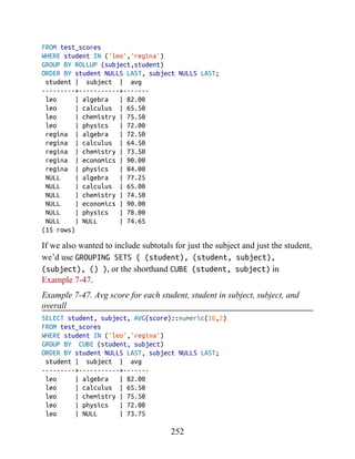
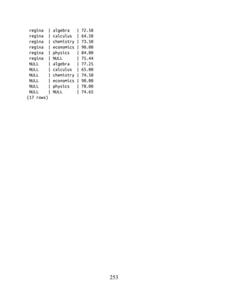
FILTER Clause for Aggregates
New in version 9.4 is the FILTER clause for aggregates, recently standardized
in ANSI SQL. This replaces the standard CASE WHEN clause for reducing the
number of rows included in an aggregation. For example, suppose you used
CASE WHEN to break out average test scores by student, as shown in
Example 7-23.
Example 7-23. CASE WHEN used in AVG
SELECT student,
232](https://image.slidesharecdn.com/postgresqlupandrunningapracticalguidetotheadvancedopensourcedatabasepdfdrive-221213051845-fb16fe5b/85/PostgreSQL_-Up-and-Running_-A-Practical-Guide-to-the-Advanced-Open-Source-Database-PDFDrive-pdf-232-320.jpg)
![percentile_cont(0.5) WITHIN GROUP (ORDER BY score) As cont_median,
percentile_disc(0.5) WITHIN GROUP (ORDER BY score) AS disc_median,
mode() WITHIN GROUP (ORDER BY score) AS mode,
COUNT(*) As num_scores
FROM test_scores
GROUP BY student
ORDER BY student;
student | cont_median | disc_median | mode | num_scores
--------+-------------+-------------+------+------------
alex | 78 | 77 | 74 | 8
leo | 72 | 72 | 72 | 8
regina | 76 | 76 | 68 | 9
sonia | 73.5 | 72 | 72 | 8
(4 rows)
Example 7-27 computes both the discrete and the continuous median score,
which could differ when students have an even number of scores.
The inputs of these functions differ from other aggregate functions. The
column being aggregated is the column in the ORDER BY clauses of the
WITHIN GROUP modifiers. The column is not direct input to the function, as
we’re used to seeing.
The percentile functions have another variant that accepts an array of
percentiles, letting you retrieve multiple percentiles all in one call.
Example 7-28 computes the median, the 60 percentile, and the highest score.
Example 7-28. Compute multiple percentiles
SELECT
student,
percentile_cont('{0.5,0.60,1}'::float[])
WITHIN GROUP (ORDER BY score) AS cont_median,
percentile_disc('{0.5,0.60,1}'::float[])
WITHIN GROUP (ORDER BY score) AS disc_median,
COUNT(*) As num_scores
FROM test_scores
GROUP BY student
ORDER BY student;
student | cont_median | disc_median | num_scores
--------+----------------+-------------+------------
alex | {78,79.2,84} | {77,79,84} | 8
235](https://image.slidesharecdn.com/postgresqlupandrunningapracticalguidetotheadvancedopensourcedatabasepdfdrive-221213051845-fb16fe5b/85/PostgreSQL_-Up-and-Running_-A-Practical-Guide-to-the-Advanced-Open-Source-Database-PDFDrive-pdf-235-320.jpg)

![SELECT * FROM select_logs_xxx('alex');
Writing SQL Aggregate Functions
Yes! In PostgreSQL you are able to author your own aggregate functions to
expand beyond the usual aggregates MIN, MA, COUNT, AVG, etc. We
demonstrate by creating an aggregate function to compute the geometric
mean. A geometric mean is the nth root of a product of n positive numbers
((x1*x2*x3...xn) ). It has various uses in finance, economics, and
statistics. A geometric mean substitutes for the more common arithmetic
mean when the numbers range across vastly different scales. A more suitable
computational formula uses logarithms to transform a multiplicative process
to an additive one (EXP(SUM(LN(x))/n)). We’ll be using this method in our
example.
To build our geometric mean aggregate, we need two subfunctions: a state
transition function to sum the logs (see Example 8-5) and a final function to
exponentiate the logs. We’ll also specify an initial condition of zero when we
assemble everything together.
Example 8-5. Geometric mean aggregate: state function
CREATE OR REPLACE FUNCTION geom_mean_state(prev numeric[2], next numeric)
RETURNS numeric[2] AS
$$
SELECT
CASE
WHEN $2 IS NULL OR $2 = 0 THEN $1
ELSE ARRAY[COALESCE($1[1],0) + ln($2), $1[2] + 1]
END;
$$
(1/n)
CREATE OR REPLACE FUNCTION select_logs_so(param_user_name varchar)
RETURNS SETOF logs AS
$$
SELECT * FROM logs WHERE user_name = $1;
$$
LANGUAGE 'sql' STABLE PARALLEL SAFE;
Call all these functions using:
265](https://image.slidesharecdn.com/postgresqlupandrunningapracticalguidetotheadvancedopensourcedatabasepdfdrive-221213051845-fb16fe5b/85/PostgreSQL_-Up-and-Running_-A-Practical-Guide-to-the-Advanced-Open-Source-Database-PDFDrive-pdf-265-320.jpg)
![CREATE OR REPLACE FUNCTION geom_mean_final(numeric[2])
RETURNS numeric AS
$$
SELECT CASE WHEN $1[2] > 0 THEN exp($1[1]/$1[2]) ELSE 0 END;
$$
LANGUAGE sql IMMUTABLE PARALLEL SAFE;
Now we stitch all the subfunctions together in our aggregate definition, as
shown in Example 8-7. (Note that our aggregate has an initial condition that
is the same data type as the one returned by our state function.)
Example 8-7. Geometric mean aggregate: assembling the pieces
CREATE AGGREGATE geom_mean(numeric) (
SFUNC=geom_mean_state,
STYPE=numeric[],
FINALFUNC=geom_mean_final,
PARALLEL = safe,
INITCOND='{0,0}'
);
Let’s take our new function for a test drive. In Example 8-8, we compute a
heuristic rating for racial diversity and list the top five most racially diverse
counties in Massachusetts.
Example 8-8. Top five most racially diverse counties using geometric mean
SELECT left(tract_id,5) As county, geom_mean(val) As div_county
FROM census.vw_facts
WHERE category = 'Population' AND short_name != 'white_alone'
LANGUAGE sql IMMUTABLE PARALLEL SAFE;
Our state transition function takes two inputs: the previous state passed in as
an array with two elements, and the next added in the summation. If the
next argument evaluates to NULL or zero, the state function returns the prior
state. Otherwise, it returns a new array in which the first element is the sum
of the logs and the second element is the running count.
We also need a final function, shown in Example 8-6, that divides the sum
from the state transition by the count.
Example 8-6. Geometric mean aggregate: final function
266](https://image.slidesharecdn.com/postgresqlupandrunningapracticalguidetotheadvancedopensourcedatabasepdfdrive-221213051845-fb16fe5b/85/PostgreSQL_-Up-and-Running_-A-Practical-Guide-to-the-Advanced-Open-Source-Database-PDFDrive-pdf-266-320.jpg)
![Imports the libraries we’ll be using.
Performs a search after concatenating the search term.
Reads the response and saves the retrieved HTML to a variable called
raw_html.
Saves the part of the raw_html that starts with <!-- docbot goes here
--> and ends just before the beginning of <!-- pgContentWrap --> into
a new variable called result.
Removes leading and trailing HTML symbols and whitespace.
Returns result.
Calling Python functions is no different from calling functions written in
other languages. In Example 8-13, we use the function we created in
Example 8-12 to output the result with three search terms.
Example 8-13. Using Python functions in a query
SELECT search_term, left(postgresql_help_search(search_term),125) AS
result
FROM (VALUES ('regexp_match'),('pg_trgm'),('tsvector')) As
x(search_term);
Recall that PL/Python is an untrusted language, without a trusted counterpart.
This means only superusers can write functions using PL/Python, and the
function can interact with the filesystem of the OS. Example 8-14 takes
advantage of the untrusted nature of PL/Python to retrieve file listings from a
directory. Keep in mind that from the perspective of the OS, a PL/Python
import urllib, re
response = urllib.urlopen(
'http://www.postgresql.org/search/?u=%2Fdocs%2Fcurrent%2F&q=' +
param_search
)
raw_html = response.read()
result =
raw_html[raw_html.find("<!-- docbot goes here -->") :
raw_html.find("<!-- pgContentWrap -->") - 1]
result = re.sub('<[^<]+?>', '', result).strip()
return result
$$
LANGUAGE plpython2u SECURITY DEFINER STABLE;
271](https://image.slidesharecdn.com/postgresqlupandrunningapracticalguidetotheadvancedopensourcedatabasepdfdrive-221213051845-fb16fe5b/85/PostgreSQL_-Up-and-Running_-A-Practical-Guide-to-the-Advanced-Open-Source-Database-PDFDrive-pdf-271-320.jpg)
![re = /S+@S+.S+/
return re.test email
$$
LANGUAGE plcoffee IMMUTABLE STRICT PARALLEL SAFE;
CoffeeScript doesn’t look all that different from JavaScript, except for the
lack of parentheses, curly braces, and semicolons. The LiveScript version
looks exactly like the CoffeeScript except with a LANGUAGE plls specifier.
Writing Aggregate Functions with PL/V8
In Examples 8-19 and 8-20, we reformulate the state transition and final
function of the geometric mean aggregate function (see “Writing SQL
Aggregate Functions”) using PL/V8.
Example 8-19. PL/V8 geometric mean aggregate: state transition function
CREATE OR REPLACE FUNCTION geom_mean_state(prev numeric[2], next numeric)
RETURNS numeric[2] AS
$$
return (next == null || next == 0) ? prev :
[(prev[0] == null)? 0: prev[0] + Math.log(next), prev[1] + 1];
$$
LANGUAGE plv8 IMMUTABLE PARALLEL SAFE;
Example 8-20. PL/V8 geometric mean aggregate: final function
CREATE OR REPLACE FUNCTION geom_mean_final(in_num numeric[2])
RETURNS numeric AS
$$
return in_num[1] > 0 ? Math.exp(in_num[0]/in_num[1]) : 0;
$$
LANGUAGE plv8 IMMUTABLE PARALLEL SAFE;
The final CREATE AGGREGATE puts all the pieces together and looks more or
less the same in all languages. Our PL/V8 variant is shown in Example 8-21.
Example 8-21. PL/V8 geometric mean aggregate: putting all the pieces
together
CREATE AGGREGATE geom_mean(numeric) (
SFUNC=geom_mean_state,
STYPE=numeric[],
276](https://image.slidesharecdn.com/postgresqlupandrunningapracticalguidetotheadvancedopensourcedatabasepdfdrive-221213051845-fb16fe5b/85/PostgreSQL_-Up-and-Running_-A-Practical-Guide-to-the-Advanced-Open-Source-Database-PDFDrive-pdf-276-320.jpg)

![CREATE INDEX idx_lu_fact_types ON census.lu_fact_types USING gin
(fact_subcats);
To test our index, we’ll execute a query to find all rows with subcats
containing “White alone” or “Asian alone.” We explicitly enabled sequential
scan even though it’s the default setting, just to be sure. The accompanying
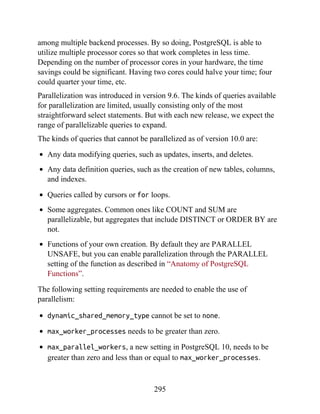
EXPLAIN output is shown in Example 9-15.
Example 9-15. Allow planner to choose sequential scan
set enable_seqscan = true;
EXPLAIN (ANALYZE)
SELECT *
FROM census.lu_fact_types
WHERE fact_subcats && '{White alone, Black alone}'::varchar[];
Seq Scan on lu_fact_types
(cost=0.00..2.85 rows=2 width=200)
actual time=0.066..0.076 rows=2 loops=1)
Filter: (fact_subcats
&& '{"White alone","Black alone"}'::character varying[])
Rows Removed by Filter: 66
Planning time: 0.182 ms
Execution time: 0.108 ms
Observe that when enable_seqscan is enabled, our index is not being used
and the planner has chosen to do a sequential scan. This could be because our
table is so small or because the index we have is no good for this query. If we
repeat the query but turn off sequential scan beforehand, as shown in
Example 9-16, we can see that we have succeeded in forcing the planner to
use the index.
Example 9-16. Disable sequential scan, coerce index use
set enable_seqscan = false;
pg_stat_statements extension described in “Gathering Statistics on
Statements”.
Let’s start off with a query against the table we created in Example 7-22.
We’ll add a GIN index on the array column. GIN indexes are among the few
indexes you can use to index arrays:
302](https://image.slidesharecdn.com/postgresqlupandrunningapracticalguidetotheadvancedopensourcedatabasepdfdrive-221213051845-fb16fe5b/85/PostgreSQL_-Up-and-Running_-A-Practical-Guide-to-the-Advanced-Open-Source-Database-PDFDrive-pdf-302-320.jpg)
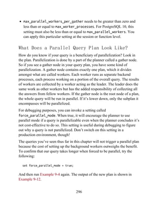
![(cost=12.02..14.04 rows=2 width=200)
(actual time=0.058..0.058 rows=2 loops=1)
Recheck Cond: (fact_subcats
&& '{"White alone","Black alone"}'::character varying[])
Heap Blocks: exact=1
-> Bitmap Index Scan on idx_lu_fact_types
(cost=0.00..12.02 rows=2 width=0)
(actual time=0.048..0.048 rows=2 loops=1)
Index Cond: (fact_subcats
&& '{"White alone","Black alone"}'::character varying[])
Planning time: 0.230 ms
Execution time: 0.119 ms
From this plan, we learn that our index can be used but ends up making the
query take longer because the cost is more than doing a sequential scan.
Therefore, under normal circumstances, the planner will opt for the sequential
scan. As we add more data to our table, we’ll probably find that the planner
changes strategies to an index scan.
In contrast to the previous example, suppose we were to write a query of the
form:
SELECT * FROM census.lu_fact_types WHERE 'White alone' =
ANY(fact_subcats);
We would discover that, regardless of how we set enable_seqscan, the
planner will always perform a sequential scan because the index we have in
place can’t service this query. So it is important to consider which indexes
will be useful and to write queries to take advantage of them. And
experiment, experiment, experiment!
Table Statistics
Despite what you might think or hope, the query planner is not a magician.
EXPLAIN (ANALYZE)
SELECT *
FROM census.lu_fact_types
WHERE fact_subcats && '{White alone, Black alone}'::varchar[];
Bitmap Heap Scan on lu_fact_types
303](https://image.slidesharecdn.com/postgresqlupandrunningapracticalguidetotheadvancedopensourcedatabasepdfdrive-221213051845-fb16fe5b/85/PostgreSQL_-Up-and-Running_-A-Practical-Guide-to-the-Advanced-Open-Source-Database-PDFDrive-pdf-303-320.jpg)
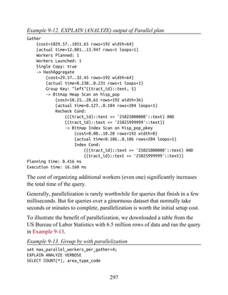
![SELECT T.fact_subcats[2], COUNT(*) As num_fact
FROM
census.facts As F
INNER JOIN
census.lu_fact_types AS T ON F.fact_type_id = T.fact_type_id
GROUP BY T.fact_subcats[2];
The second time you run the query, you should notice at least a 10%
performance speed increase and should see the following cached in the
buffer:
relname | dirty_buffers | num_buffers
--------------+---------------+------------
facts | 0 | 736
lu_fact_types | 0 | 4
The more onboard memory you have dedicated to the cache, the more room
you’ll have to cache data. You can set the amount of dedicated memory by
changing the shared_buffers setting in postgresql.conf. Don’t go
overboard; raising shared_buffers too much will bloat your cache, leading
to more time wasted scanning the cache.
Nowadays, there’s no shortage of onboard memory. You can take advantage
of this by precaching commonly used tables using an extension called
pg_prewarm. pg_prewarm lets you prime your PostgreSQL by loading data
from commonly used tables into memory so that the first user to hit the
database can experience the same performance boost offered by caching as
later users. A good article that describes this feature is Prewarming Relational
Data.
308](https://image.slidesharecdn.com/postgresqlupandrunningapracticalguidetotheadvancedopensourcedatabasepdfdrive-221213051845-fb16fe5b/85/PostgreSQL_-Up-and-Running_-A-Practical-Guide-to-the-Advanced-Open-Source-Database-PDFDrive-pdf-308-320.jpg)
![Bruce Momjian|EnterpriseDB
Example 10-1. Make a foreign table from a delimited file
CREATE FOREIGN TABLE staging.devs (developer VARCHAR(150), company
VARCHAR(150))
SERVER my_server
OPTIONS (
format 'csv',
header 'true',
filename '/postgresql_book/ch10/devs.psv',
delimiter '|',
null ''
);
In our example, even though we’re registering a pipe-delimited file, we still
use the csv option. A CSV file, as far as FDW is concerned, represents a file
delimited by any specified character.
When the setup is finished, you can finally query your pipe-delimited file
directly:
SELECT * FROM staging.devs WHERE developer LIKE 'T%';
Once you no longer need the foreign table, drop it using:
DROP FOREIGN TABLE staging.devs;
Querying Flat Files as Jagged Arrays
Often, flat files have a different number of columns on each line and could
include multiple header and footer rows. Our favorite FDW for handling
these files is file_textarray_fdw. This wrapper can handle any kind of
delimited flat file, even if the number of elements vary from row to row, by
treating each row as a text array (text[]).
Unfortunately, file_textarray_fdw is not part of the core PostgreSQL, so
you’ll need to compile it yourself. First, install PostgreSQL with PostgreSQL
development headers. Then download the file_textarray_fdw source code
323](https://image.slidesharecdn.com/postgresqlupandrunningapracticalguidetotheadvancedopensourcedatabasepdfdrive-221213051845-fb16fe5b/85/PostgreSQL_-Up-and-Running_-A-Practical-Guide-to-the-Advanced-Open-Source-Database-PDFDrive-pdf-323-320.jpg)
![CREATE FOREIGN TABLE staging.factfinder_array (x text[])
SERVER file_taserver
OPTIONS (
format 'csv',
filename '/postgresql_book/ch10/DEC_10_SF1_QTH1_with_ann.csv',
header 'false',
delimiter ',',
quote '"',
encoding 'latin1',
null ''
);
Our example CSV begins with eight header rows and has more columns than
we care to count. When the setup is finished, you can finally query our
delimited file directly. The following query will give us the names of the
header rows where the first column of the header is GEO.id:
from the Adunstan GitHub site. There is a different branch for each version
of PostgreSQL, so make sure to pick the right one. Once you’ve compiled the
code, install it as an extension, as you would any other FDW.
If you are on Linux/Unix, it’s an easy compile if you have the postgresql-
dev package installed. We did the work of compiling for Windows; you can
download our binaries from one of the following links: one for Windows
32/64 9.4 FDWs, and another for Windows 32/64 9.5 and 32/64 9.6 FDWs.
The first step to perform after you have installed an FDW is to create an
extension in your database:
CREATE EXTENSION file_textarray_fdw;
Then create a foreign server as you would with any FDW:
CREATE SERVER file_taserver FOREIGN DATA WRAPPER file_textarray_fdw;
Next, register the tables. You can place foreign tables in any schema you
want. In Example 10-2, we use our staging schema again.
Example 10-2. Make a file text array foreign table from a delimited file
324](https://image.slidesharecdn.com/postgresqlupandrunningapracticalguidetotheadvancedopensourcedatabasepdfdrive-221213051845-fb16fe5b/85/PostgreSQL_-Up-and-Running_-A-Practical-Guide-to-the-Advanced-Open-Source-Database-PDFDrive-pdf-324-320.jpg)
![SELECT unnest(x) FROM staging.factfinder_array WHERE x[1] = 'GEO.id'
This next query will give us the first two columns of our data:
SELECT x[1] As geo_id, x[2] As tract_id
FROM staging.factfinder_array WHERE x[1] ~ '[0-9]+';
Querying Other PostgreSQL Servers
The PostgreSQL FDW, postgres_fdw, is packaged with most distributions
of PostgreSQL since PostgreSQL 9.3. This FDW allows you to read as well
as push updates to other PostgreSQL servers, even different versions.
Start by installing the FDW for the PostgreSQL server in a new database:
CREATE EXTENSION postgres_fdw;
Next, create a foreign server:
CREATE SERVER book_server
FOREIGN DATA WRAPPER postgres_fdw
OPTIONS (host 'localhost', port '5432', dbname 'postgresql_book');
If you need to change or add connection options to the foreign server after
creation, you can use the ALTER SERVER command. For example, if you
needed to change the server you are pointing to, you could enter:
ALTER SERVER book_server OPTIONS (SET host 'prod');
WARNING
Changes to connection settings such as the host, port, and database do not take
effect until a new session is created. This is because the connection is opened
on first use and is kept open.
Next, create a user, mapping its public role to a role on the foreign server:
325](https://image.slidesharecdn.com/postgresqlupandrunningapracticalguidetotheadvancedopensourcedatabasepdfdrive-221213051845-fb16fe5b/85/PostgreSQL_-Up-and-Running_-A-Practical-Guide-to-the-Advanced-Open-Source-Database-PDFDrive-pdf-325-320.jpg)
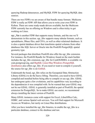
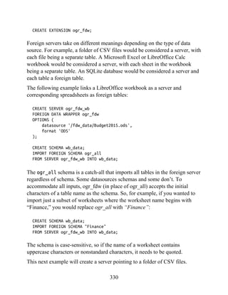
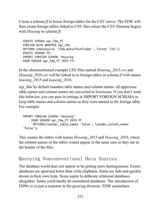
![CREATE FOREIGN TABLE www_fdw_google_search (
q text,
GsearchResultClass text,
unescapedUrl text,
url text,
visibleUrl text,
cacheUrl text,
title text,
content text
) SERVER www_fdw_server_google_search;
The user mapping doesn’t assign any rights. You still need to grant rights
before being able to query the foreign table:
GRANT SELECT ON TABLE www_fdw_google_search TO public;
Now comes the fun part. We search with the term New in PostgreSQL 9.4
and mix in a bit of regular expression goodness to strip off HTML tags:
SELECT regexp_replace(title,E'(?x)(< [^>]*? >)','','g') As title
FROM www_fdw_google_search
WHERE q = 'New in PostgreSQL 10'
LIMIT 2;
Voilà! We have our response:
title
---------------------
PostgreSQL 10 Roadmap
PostgreSQL: Roadmap
(2 rows)
333](https://image.slidesharecdn.com/postgresqlupandrunningapracticalguidetotheadvancedopensourcedatabasepdfdrive-221213051845-fb16fe5b/85/PostgreSQL_-Up-and-Running_-A-Practical-Guide-to-the-Advanced-Open-Source-Database-PDFDrive-pdf-333-320.jpg)
![This appendix summarizes indispensable command-line tools packaged with
PostgreSQL server. We discussed them at length in the book. Here we list
their help messages. We hope to save you a bit of time with their inclusion
and perhaps make this book a not-so-strange bedfellow.
Database Backup Using pg_dump
Use pg_dump to back up all or part of a database. Backup file formats
available are TAR, compressed (PostgreSQL custom format), plain text, and
plain-text SQL. Plain-text backup can copy psql-specific commands;
therefore, restore by running the file within psql. A plain-text SQL backup is
merely a file with standard SQL CREATE and INSERT commands. To restore,
you can run the file using psql or pgAdmin. Example B-1 shows the pg_dump
help output. For full coverage of pg_dump usage, see “Selective Backup
Using pg_dump”.
Example B-1. pg_dump help
pg_dump --help
pg_dump dumps a database as a text file or to other formats.
Usage:
pg_dump [OPTION]... [DBNAME]
General options:
-f, --file=FILENAME output file or directory name
-F, --format=c|d|t|p output file format (custom, directory, tar,
plain
text)
-j, --jobs=NUM use this many parallel jobs to dump
-v, --verbose verbose mode
-Z, --compress=0-9 compression level for compressed formats
Appendix B. PostgreSQL
Packaged Command-Line Tools
340](https://image.slidesharecdn.com/postgresqlupandrunningapracticalguidetotheadvancedopensourcedatabasepdfdrive-221213051845-fb16fe5b/85/PostgreSQL_-Up-and-Running_-A-Practical-Guide-to-the-Advanced-Open-Source-Database-PDFDrive-pdf-340-320.jpg)
![-f, --file=FILENAME output file name
-v, --verbose verbose mode
-V, --version output version information, then exit
--lock-wait-timeout=TIMEOUT fail after waiting TIMEOUT for a table lock
-?, --help show this help, then exit
Options controlling the output content:
-a, --data-only dump only the data, not the schema
-c, --clean clean (drop) databases before recreating
-g, --globals-only dump only global objects, no databases
-o, --oids include OIDs in dump
-O, --no-owner skip restoration of object ownership
-r, --roles-only dump only roles, no databases or tablespaces
-s, --schema-only dump only the schema, no data
-S, --superuser=NAME superuser user name to use in the dump
-t, --tablespaces-only dump only tablespaces, no databases or roles
-x, --no-privileges do not dump privileges (grant/revoke)
--binary-upgrade for use by upgrade utilities only
--column-inserts dump data as INSERT commands with column
names
--disable-dollar-quoting disable dollar quoting, use SQL standard
quoting
--disable-triggers disable triggers during data-only restore
--inserts dump data as INSERT commands, rather than
COPY
--no-publications do not dump publications
--no-security-labels do not dump security label assignments
--no-subscriptions do not dump subscriptions
--no-sync do not wait for changes to be written safely
to disk
--no-tablespaces do not dump tablespace assignments
--no-unlogged-table-data do not dump unlogged table data
--no-role-passwords do not dump passwords for roles
--quote-all-identifiers quote all identifiers, even if not keywords
--use-set-session-authorization
use SET SESSION AUTHORIZATION commands instead o
ALTER OWNER commands to set ownership
Connection options:
Usage:
pg_dumpall [OPTION]...
General options:
343](https://image.slidesharecdn.com/postgresqlupandrunningapracticalguidetotheadvancedopensourcedatabasepdfdrive-221213051845-fb16fe5b/85/PostgreSQL_-Up-and-Running_-A-Practical-Guide-to-the-Advanced-Open-Source-Database-PDFDrive-pdf-343-320.jpg)
![-d, --dbname=CONNSTR connect using connection string
-h, --host=HOSTNAME database server host or socket directory
-l, --database=DBNAME alternative default database
-p, --port=PORT database server port number
-U, --username=NAME connect as specified database user
-w, --no-password never prompt for password
-W, --password force password prompt (should happen
automatically)
--role=ROLENAME do SET ROLE before dump
If -f/--file is not used, then the SQL script will be written to the
standard
output.
New in PostgreSQL 10.
Database Restore: pg_restore
Use pg_restore to restore backup files in tar, custom, or directory formats
created using pg_dump. Example B-3 shows the pg_restore help output. See
“Restoring Data” for more examples.
Example B-3. pg_restore help
pg_restore --help
pg_restore restores a PostgreSQL database from an archive created by
pg_dump.
Usage:
pg_restore [OPTION]... [FILE]
General options:
-d, --dbname=NAME connect to database name
-f, --file=FILENAME output file name
-F, --format=c|d|t backup file format (should be automatic)
-l, --list print summarized TOC of the archive
-v, --verbose verbose mode
-V, --version output version information, then exit
-?, --help show this help, then exit
Options controlling the restore:
-a, --data-only restore only the data, no schema
-c, --clean clean (drop) database objects before
344](https://image.slidesharecdn.com/postgresqlupandrunningapracticalguidetotheadvancedopensourcedatabasepdfdrive-221213051845-fb16fe5b/85/PostgreSQL_-Up-and-Running_-A-Practical-Guide-to-the-Advanced-Open-Source-Database-PDFDrive-pdf-344-320.jpg)
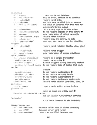
![-w, --no-password never prompt for password
-W, --password force password prompt (should happen
automatically)
--role=ROLENAME do SET ROLE before restore
New features introduced in PostgreSQL 10.
New features introduced in PostgreSQL 9.6. Prior to 9.6, the -t option
matched only tables. In 9.6 it was changed to also match foreign tables,
views, materialized views, and sequences.
New features introduced in PostgreSQL 9.5.
psql Interactive Commands
Example B-4 lists commands available in psql when you launch an
interactive session. For examples of usage, see “Environment Variables” and
“Interactive versus Noninteractive psql”.
Example B-4. Getting a list of interactive psql commands
?
General
copyright show PostgreSQL usage and distribution terms
errverbose show most recent error message at maximum
verbosity
g [FILE] or ; execute query (and send results to file or
|pipe)
gexec execute query, then execute each value in its
result
gset [PREFIX] execute query and store results in psql
variables
h [NAME] help on syntax of SQL commands, * for all
commands
gx [FILE] as g, but forces expanded output mode
q quit psql
crosstabview [COLUMNS] execute query and display results in crosstab
watch [SEC] execute query every SEC seconds
Help
? [commands] show help on backslash commands
? options show help on psql command-line options
? variables show help on special variables
h [NAME] help on syntax of SQL commands, * for all
346](https://image.slidesharecdn.com/postgresqlupandrunningapracticalguidetotheadvancedopensourcedatabasepdfdrive-221213051845-fb16fe5b/85/PostgreSQL_-Up-and-Running_-A-Practical-Guide-to-the-Advanced-Open-Source-Database-PDFDrive-pdf-346-320.jpg)
![ef [FUNCNAME [LINE]] edit function definition with external editor
ev [VIEWNAME [LINE]] edit view definition with external editor
p show the contents of the query buffer
r reset (clear) the query buffer
w FILE write query buffer to file
Input/Output
copy ... perform SQL COPY with data stream to the client
host
echo [STRING] write string to standard output
i FILE execute commands from file
ir FILE as i, but relative to location of current script
o [FILE] send all query results to file or |pipe
qecho [STRING] write string to query output stream (see o)
Conditional
if EXPR begin conditional block
elif EXPR alternative within current conditional block
else final alternative within current conditional
block
endif end conditional block
Informational
(options: S = show system objects, + = additional detail)
d[S+] list tables, views, and sequences
d[S+] NAME describe table, view, sequence, or index
da[S] [PATTERN] list aggregates
dA[+] [PATTERN] list access methods
db[+] [PATTERN] list tablespaces
dc[S] [PATTERN] list conversions
dC [PATTERN] list casts
dd[S] [PATTERN] show comments on objects
ddp [PATTERN] list default privileges
dD[S] [PATTERN] list domains
det[+] [PATTERN] list foreign tables
des[+] [PATTERN] list foreign servers
deu[+] [PATTERN] list user mappings
dew[+] [PATTERN] list foreign-data wrappers
df[antw][S+] [PATRN] list [only agg/normal/trigger/window] functions
dF[+] [PATTERN] list text search configurations
dFd[+] [PATTERN] list text search dictionaries
dFp[+] [PATTERN] list text search parsers
commands
Query Buffer
e [FILE] [LINE] edit the query buffer (or file) with external
editor
347](https://image.slidesharecdn.com/postgresqlupandrunningapracticalguidetotheadvancedopensourcedatabasepdfdrive-221213051845-fb16fe5b/85/PostgreSQL_-Up-and-Running_-A-Practical-Guide-to-the-Advanced-Open-Source-Database-PDFDrive-pdf-347-320.jpg)
![dFt[+] [PATTERN] list text search templates
dg[S+] [PATTERN] list roles
di[S+] [PATTERN] list indexes
dl list large objects, same as lo_list
dL[S+] [PATTERN] list procedural languages
dm[S+] [PATTERN] list materialized views
dn[S+] [PATTERN] list schemas
do[S] [PATTERN] list operators
dO[S+] [PATTERN] list collations
dp [PATTERN] list table, view, and sequence access privileges
drds [PATRN1 [PATRN2]] list per-database role settings
dRp[+] [PATTERN] list replication publications
dRs[+] [PATTERN] list replication subscriptions
ds[S+] [PATTERN] list sequences
dt[S+] [PATTERN] list tables
dT[S+] [PATTERN] list data types
du[S+] [PATTERN] list roles
dv[S+] [PATTERN] list views
dE[S+] [PATTERN] list foreign tables
dx[+] [PATTERN] list extensions
dy [PATTERN] list event triggers
l[+] list databases
sf[+] FUNCNAME show a function's definition
sv[+] VIEWNAME show a view's definition
z [PATTERN] same as dp
Formatting
a toggle between unaligned and aligned output mode
C [STRING] set table title, or unset if none
f [STRING] show or set field separator for unaligned query
output
H toggle HTML output mode (currently off)
pset NAME [VALUE] set table output option
(NAME :=
{format|border|expanded|fieldsep|fieldsep_zero
| footer|null|
numericlocale|recordsep|tuples_only|title|tableattr|pager
|unicode_border_linestyle|unicode_column_linestyle
|unicode_header_linestyle
})
t [on|off] show only rows (currently off)
T [STRING] set HTML <table> tag attributes, or unset if
none
348](https://image.slidesharecdn.com/postgresqlupandrunningapracticalguidetotheadvancedopensourcedatabasepdfdrive-221213051845-fb16fe5b/85/PostgreSQL_-Up-and-Running_-A-Practical-Guide-to-the-Advanced-Open-Source-Database-PDFDrive-pdf-348-320.jpg)
![x [on|off] toggle expanded output (currently off)
Connection
c[onnect] {[DBNAME|- USER|- HOST|- PORT|-] | conninfo}
connect to new database (currently "postgres")
encoding [ENCODING] show or set client encoding
password [USERNAME] securely change the password for a user
conninfo display information about current connection
Operating System
cd [DIR] change the current working directory
setenv NAME [VALUE] set or unset environment variable
timing [on|off] toggle timing of commands (currently off)
! [COMMAND] execute command in shell or start interactive
shell
New features introduced in PostgreSQL 10. All conditional options are
new.
New features introduced in PostgreSQL 9.6.
New feature introduced in PostgreSQL 9.5.
psql Noninteractive Commands
Example B-5 shows the noninteractive commands help screen. Examples of
their usage are covered in “Interactive versus Noninteractive psql”.
Example B-5. psql basic help screen
psql --help
psql is the PostgreSQL interactive terminal.
Usage:
psql [OPTION]... [DBNAME [USERNAME]]
General options:
-c, --command=COMMAND run only single command (SQL or internal) and
exit
-d, --dbname=DBNAME database name to connect to
-f, --file=FILENAME execute commands from file, then exit
-l, --list list available databases, then exit
-v, --set=, --variable=NAME=VALUE
set psql variable NAME to VALUE
(e.g., -v ON_ERROR_STOP=1)
-X, --no-psqlrc do not read startup file (~/.psqlrc)
349](https://image.slidesharecdn.com/postgresqlupandrunningapracticalguidetotheadvancedopensourcedatabasepdfdrive-221213051845-fb16fe5b/85/PostgreSQL_-Up-and-Running_-A-Practical-Guide-to-the-Advanced-Open-Source-Database-PDFDrive-pdf-349-320.jpg)
![-1 ("one"), --single-transaction
execute command file as a single transaction
-?, --help[=options] show this help, then exit
--help=commands list backslash commands, then exit
--help=variables list special variables, then exit
--version output version information, then exit
Input and output options:
-a, --echo-all echo all input from script
-b, --echo-errors echo failed commands
-e, --echo-queries echo commands sent to server
-E, --echo-hidden display queries that internal commands generate
-L, --log-file=FILENAME send session log to file
-n, --no-readline disable enhanced command-line editing (readline)
-o, --output=FILENAME send query results to file (or |pipe)
-q, --quiet run quietly (no messages, only query output)
-s, --single-step single-step mode (confirm each query)
-S, --single-line single-line mode (end of line terminates SQL
command)
Output format options:
-A, --no-align unaligned table output mode
-F, --field-separator=STRING
set field separator (default: "|")
-H, --html HTML table output mode
-P, --pset=VAR[=ARG] set printing option VAR to ARG (see pset
command)
-R, --record-separator=STRING
set record separator (default: newline)
-t, --tuples-only print rows only
-T, --table-attr=TEXT set HTML table tag attributes (e.g., width,
border)
-x, --expanded turn on expanded table output
-z, --field-separator-zero
set field separator to zero byte
-0, --record-separator-zero
set record separator to zero byte
Connection options:
-h, --host=HOSTNAME database server host or socket directory
-p, --port=PORT database server port (default: "5432")
-U, --username=USERNAME database user name
350](https://image.slidesharecdn.com/postgresqlupandrunningapracticalguidetotheadvancedopensourcedatabasepdfdrive-221213051845-fb16fe5b/85/PostgreSQL_-Up-and-Running_-A-Practical-Guide-to-the-Advanced-Open-Source-Database-PDFDrive-pdf-350-320.jpg)