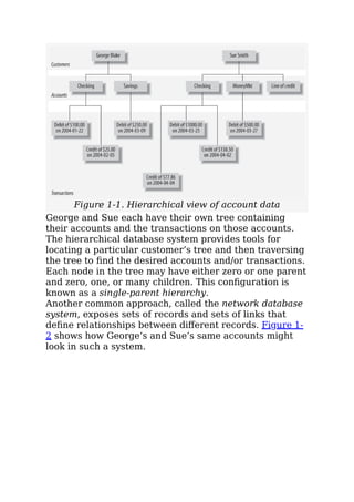
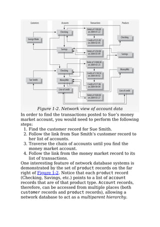
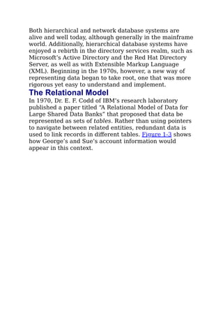
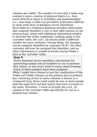
This document provides an overview and history of databases and the SQL language. It discusses early non-relational database systems that stored data hierarchically or as networks, and introduces Dr. E.F. Codd who in 1970 proposed representing data as sets of tables, known as the relational model. The remainder of the document outlines the structure and contents of the book "Learning SQL" which teaches the SQL language for querying and manipulating data in relational database systems.


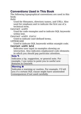


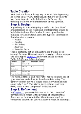


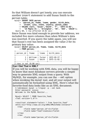


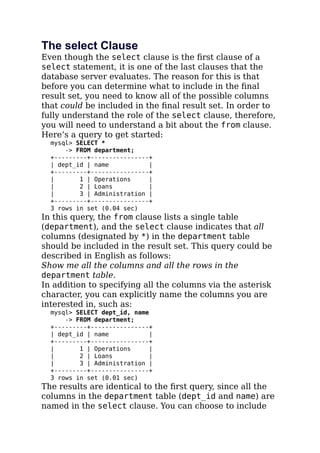


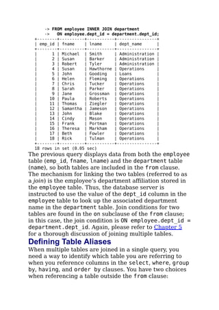


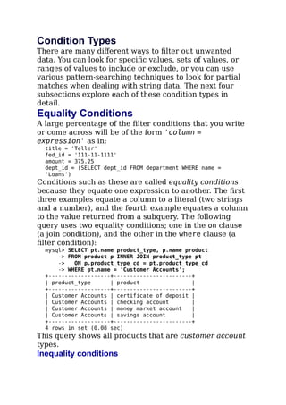


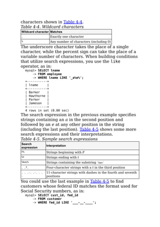

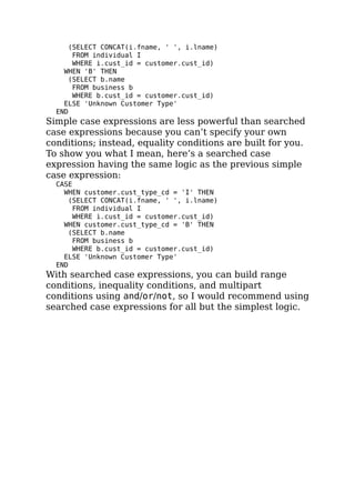
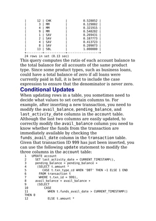
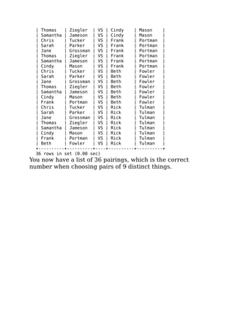
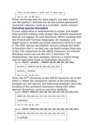
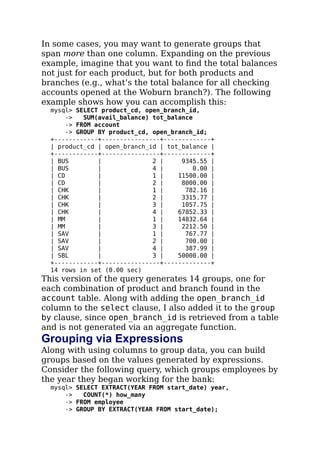
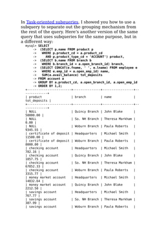
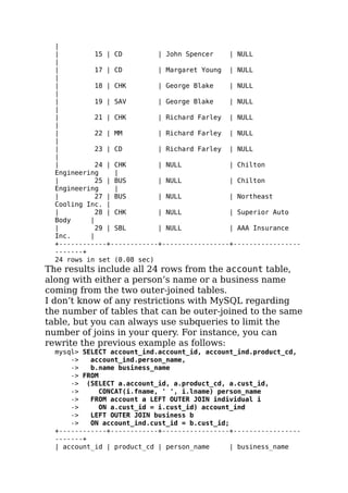
![the MySQL implementation of regular expressions:
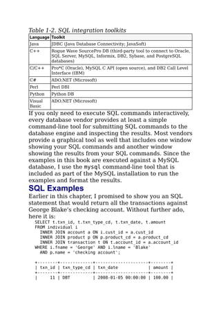
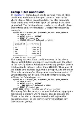
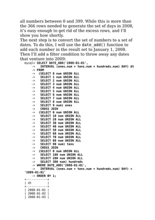
mysql> SELECT emp_id, fname, lname
-> FROM employee
-> WHERE lname REGEXP '^[FG]';
+--------+-------+----------+
| emp_id | fname | lname |
+--------+-------+----------+
| 5 | John | Gooding |
| 6 | Helen | Fleming |
| 9 | Jane | Grossman |
| 17 | Beth | Fowler |
+--------+-------+----------+
4 rows in set (0.00 sec)
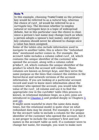
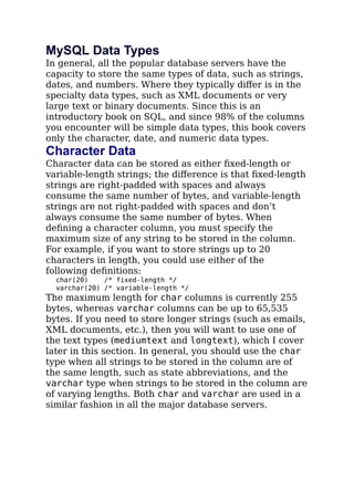
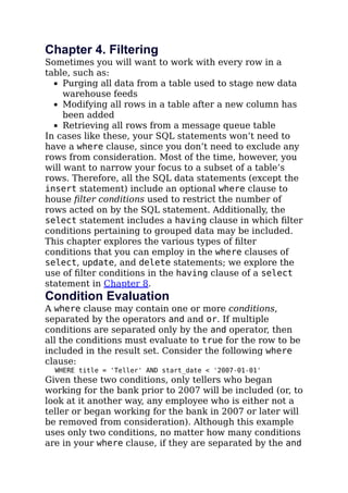
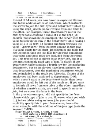
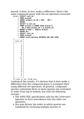
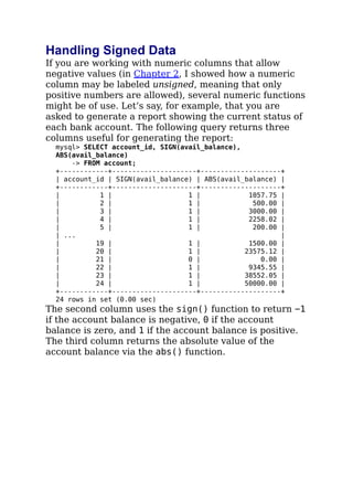
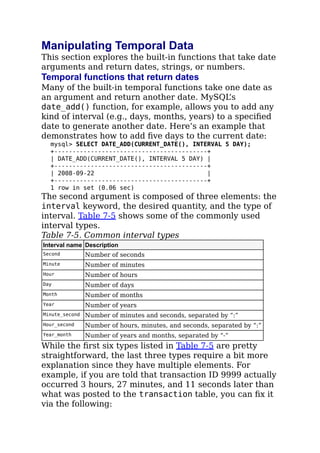
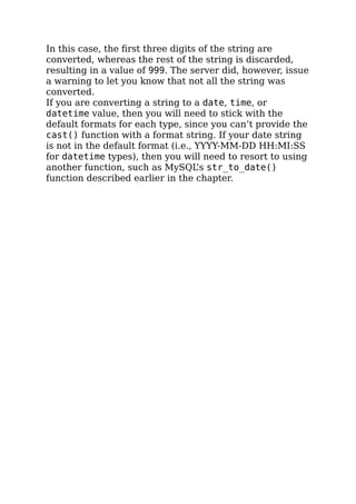
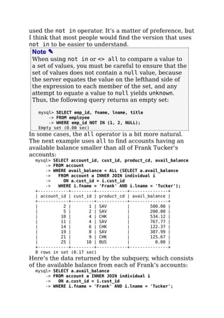
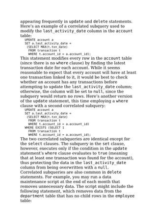
The regexp operator takes a regular expression ('^[FG]'
in this example) and applies it to the expression on the
lefthand side of the condition (the column lname). The
query now contains a single condition using a regular
expression rather than two conditions using wildcard
characters.
Oracle Database and Microsoft SQL Server also support
regular expressions. With Oracle Database, you would
use the regexp_like function instead of the regexp
operator shown in the previous example, whereas SQL
Server allows regular expressions to be used with the
like operator.](https://image.slidesharecdn.com/learningsqlbyalanbeaulieu-231102075622-ef996832/85/_Learning-SQL_-by-Alan-Beaulieu-pdf-115-320.jpg)


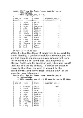


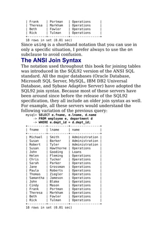


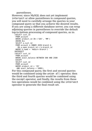


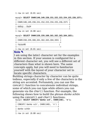


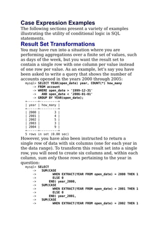
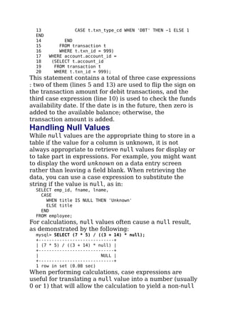
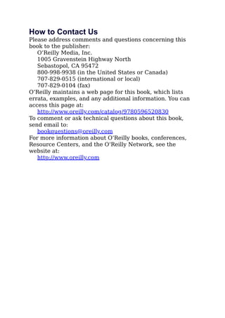
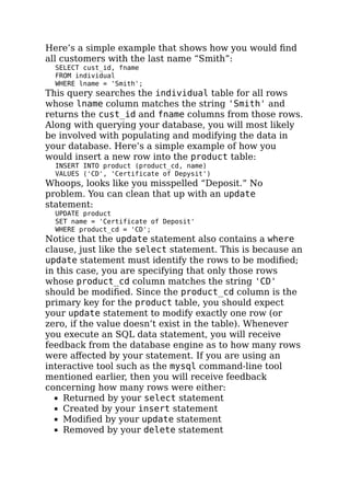
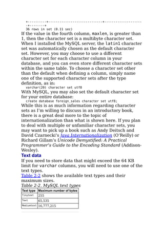
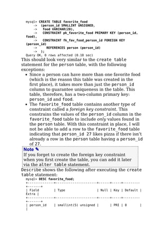
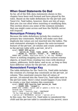
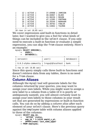
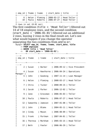
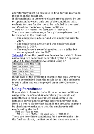
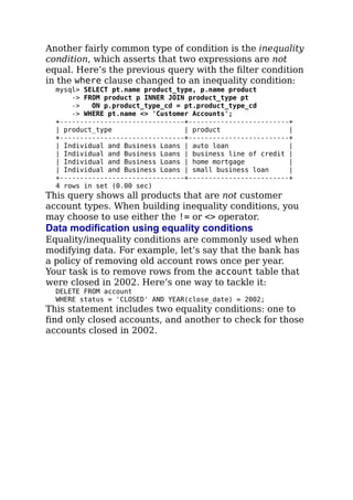
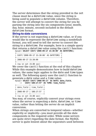
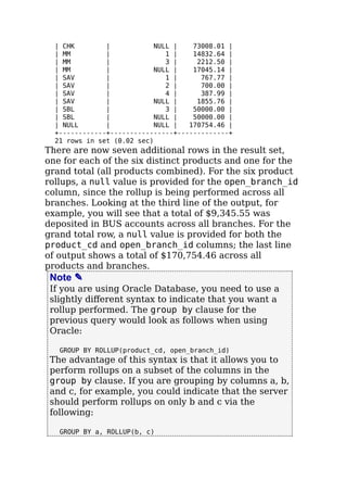
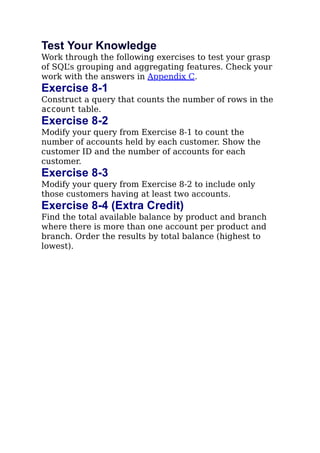
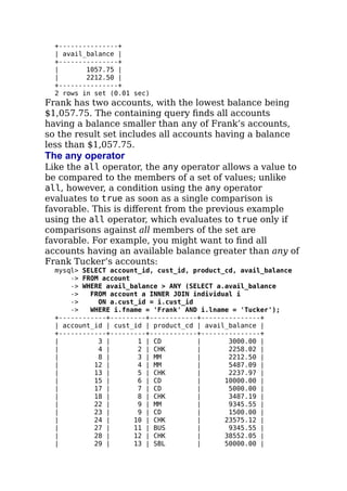
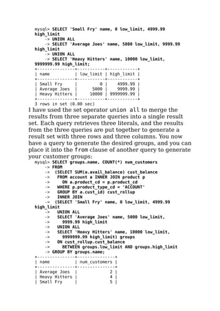
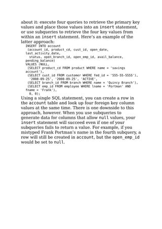
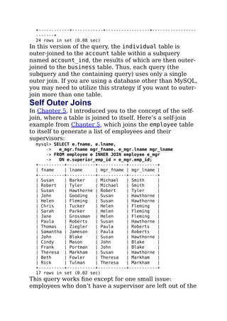
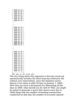
![Working with Temporal Data
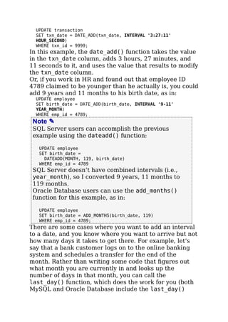
Of the three types of data discussed in this chapter
(character, numeric, and temporal), temporal data is the
most involved when it comes to data generation and
manipulation. Some of the complexity of temporal data is
caused by the myriad ways in which a single date and
time can be described. For example, the date on which I
wrote this paragraph can be described in all the
following ways:
Wednesday, September 17, 2008
9/17/2008 2:14:56 P.M. EST
9/17/2008 19:14:56 GMT
2612008 (Julian format)
Star date [−4] 85712.03 14:14:56 (Star Trek format)
While some of these differences are purely a matter of
formatting, most of the complexity has to do with your
frame of reference, which we explore in the next section.
Dealing with Time Zones
Because people around the world prefer that noon
coincides roughly with the sun’s peak at their location,
there has never been a serious attempt to coerce
everyone to use a universal clock. Instead, the world has
been sliced into 24 imaginary sections, called time zones;
within a particular time zone, everyone agrees on the
current time, whereas people in different time zones do
not. While this seems simple enough, some geographic
regions shift their time by one hour twice a year
(implementing what is known as daylight saving time)
and some do not, so the time difference between two
points on Earth might be four hours for one half of the
year and five hours for the other half of the year. Even
within a single time zone, different regions may or may
not adhere to daylight saving time, causing different
clocks in the same time zone to agree for one half of the
year but be one hour different for the rest of the year.
While the computer age has exacerbated the issue,
people have been dealing with time zone differences
since the early days of naval exploration. To ensure a](https://image.slidesharecdn.com/learningsqlbyalanbeaulieu-231102075622-ef996832/85/_Learning-SQL_-by-Alan-Beaulieu-pdf-187-320.jpg)


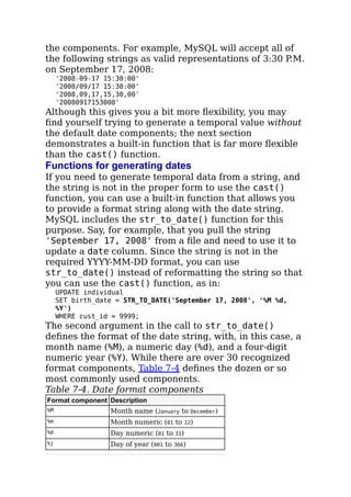


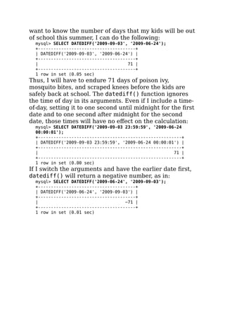


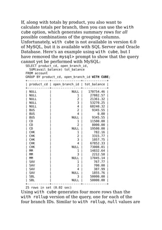

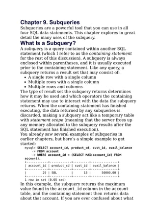


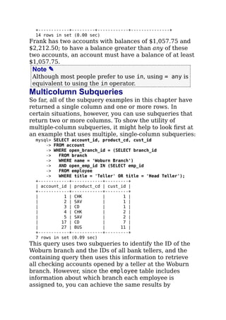


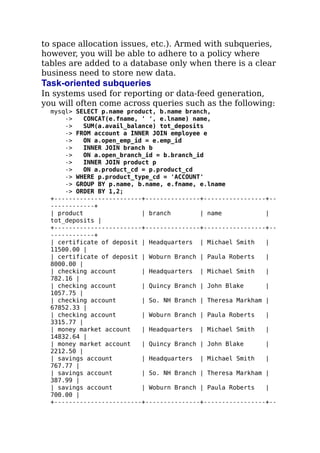


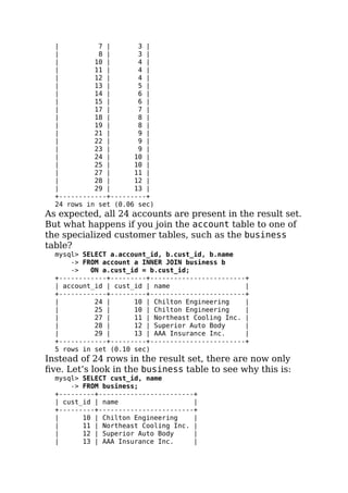


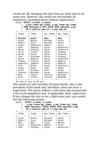


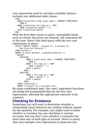
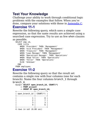
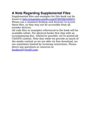
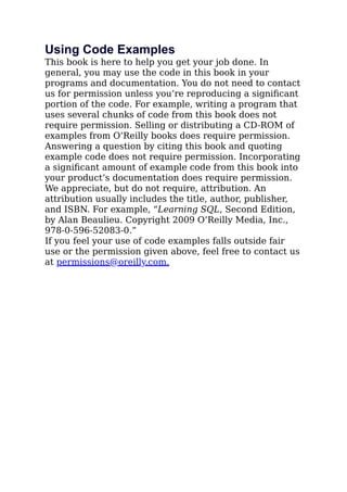
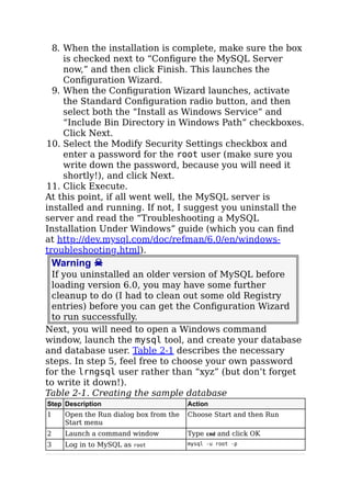
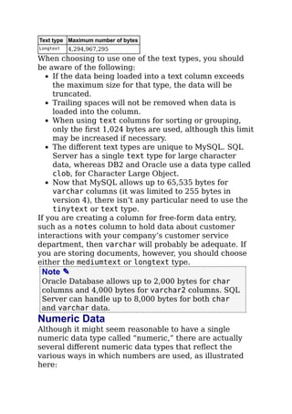
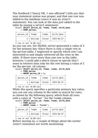
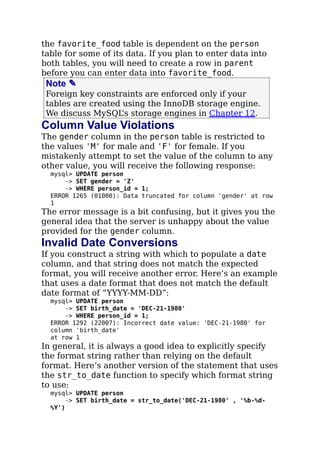
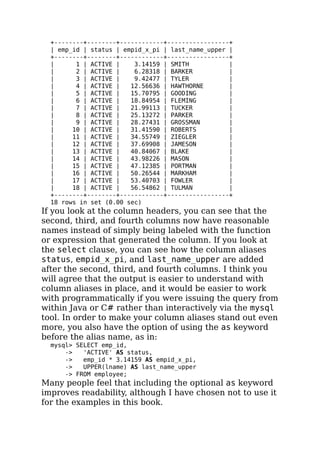
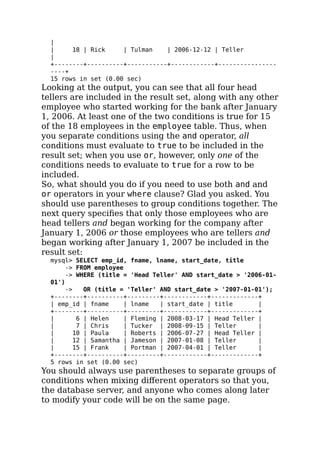
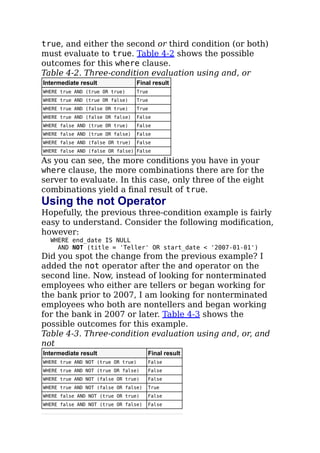
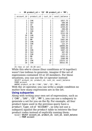
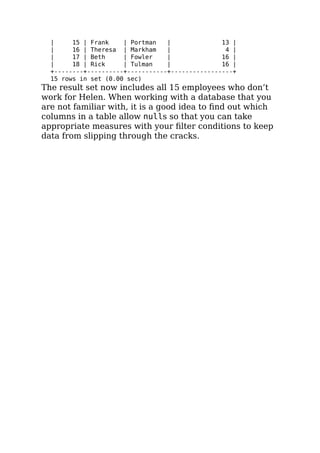
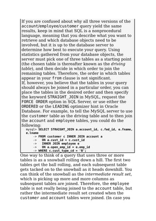
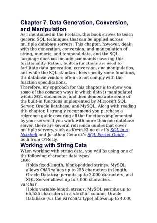
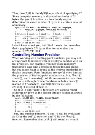
![The Case Expression
All of the major database servers include built-in
functions designed to mimic the if-then-else statement
found in most programming languages (examples include
Oracle’s decode() function, MySQL’s if() function, and
SQL Server’s coalesce() function). Case expressions are
also designed to facilitate if-then-else logic but enjoy two
advantages over built-in functions:
The case expression is part of the SQL standard
(SQL92 release) and has been implemented by
Oracle Database, SQL Server, MySQL, Sybase,
PostgreSQL, IBM UDB, and others.
Case expressions are built into the SQL grammar and
can be included in select, insert, update, and
delete statements.
The next two subsections introduce the two different
types of case expressions, and then I show you some
examples of case expressions in action.
Searched Case Expressions
The case expression demonstrated earlier in the chapter
is an example of a searched case expression, which has
the following syntax:
CASE
WHEN C1 THEN E1
WHEN C2 THEN E2
...
WHEN CN THEN EN
[ELSE ED]
END
In the previous definition, the symbols C1, C2,..., CN
represent conditions, and the symbols E1, E2,..., EN
represent expressions to be returned by the case
expression. If the condition in a when clause evaluates to
true, then the case expression returns the corresponding
expression. Additionally, the ED symbol represents the
default expression, which the case expression returns if
none of the conditions C1, C2,..., CN evaluate to true (the
else clause is optional, which is why it is enclosed in
square brackets). All the expressions returned by the](https://image.slidesharecdn.com/learningsqlbyalanbeaulieu-231102075622-ef996832/85/_Learning-SQL_-by-Alan-Beaulieu-pdf-286-320.jpg)
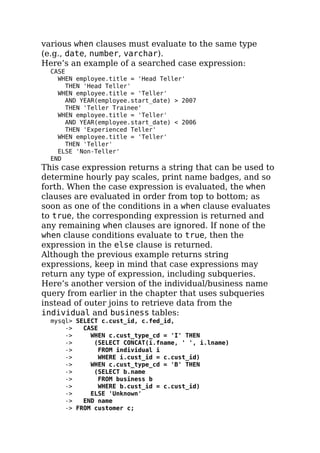
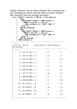
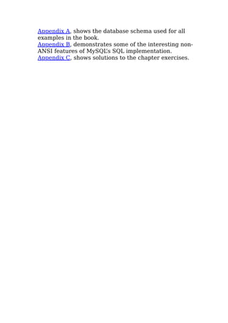
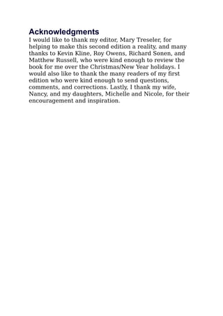
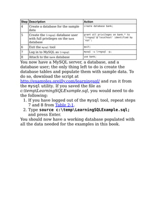
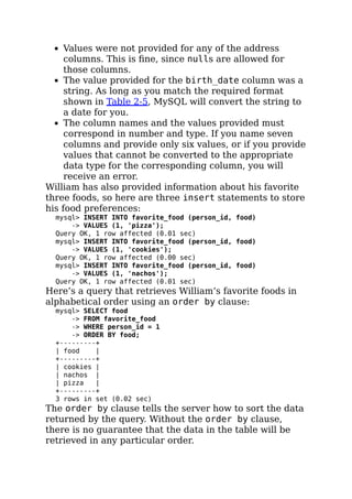
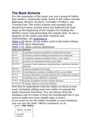
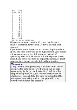
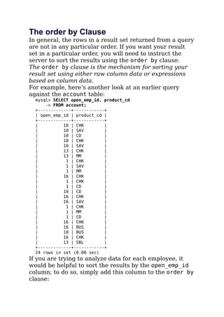
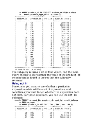
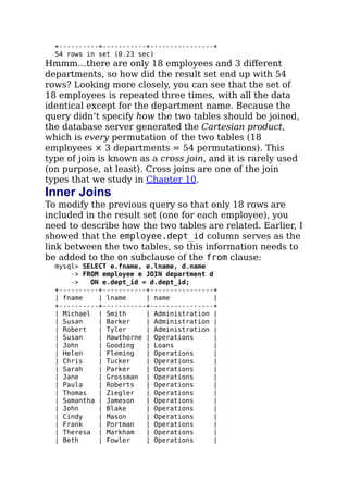
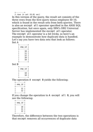
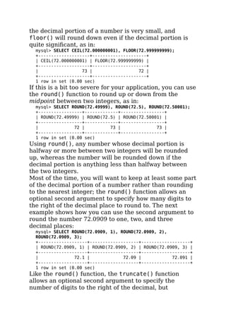
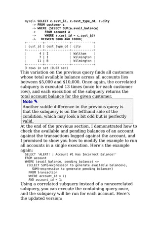
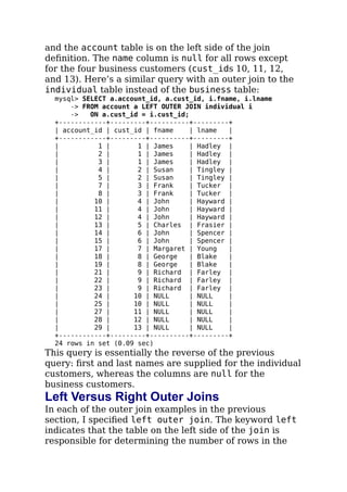
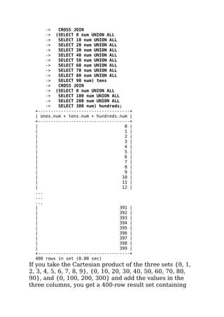
![+---------+-------------+------------------------+
| cust_id | fed_id | name |
+---------+-------------+------------------------+
| 1 | 111-11-1111 | James Hadley |
| 2 | 222-22-2222 | Susan Tingley |
| 3 | 333-33-3333 | Frank Tucker |
| 4 | 444-44-4444 | John Hayward |
| 5 | 555-55-5555 | Charles Frasier |
| 6 | 666-66-6666 | John Spencer |
| 7 | 777-77-7777 | Margaret Young |
| 8 | 888-88-8888 | Louis Blake |
| 9 | 999-99-9999 | Richard Farley |
| 10 | 04-1111111 | Chilton Engineering |
| 11 | 04-2222222 | Northeast Cooling Inc. |
| 12 | 04-3333333 | Superior Auto Body |
| 13 | 04-4444444 | AAA Insurance Inc. |
+---------+-------------+------------------------+
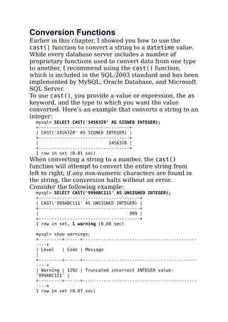
13 rows in set (0.01 sec)
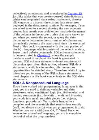
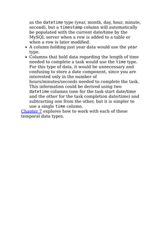
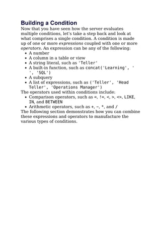
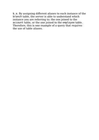
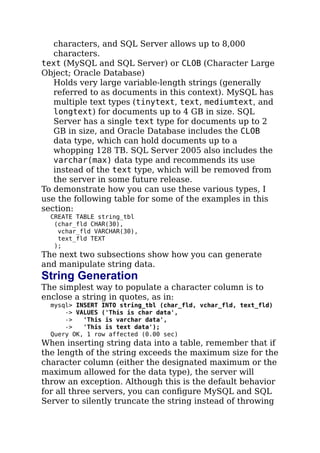
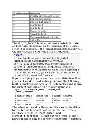
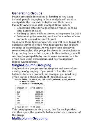
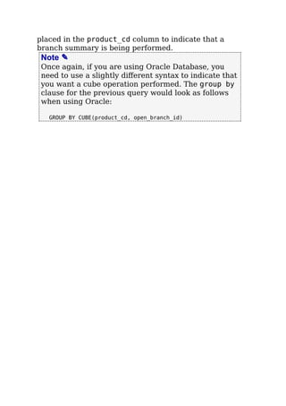
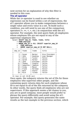
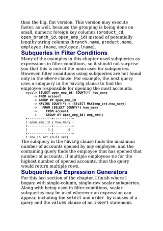
This version of the query includes only the customer
table in the from clause and uses correlated subqueries
to retrieve the appropriate name for each customer. I
prefer this version over the outer join version from
earlier in the chapter, since the server reads from the
individual and business tables only as needed instead
of always joining all three tables.
Simple Case Expressions
The simple case expression is quite similar to the
searched case expression but is a bit less flexible. Here’s
the syntax:
CASE V0
WHEN V1 THEN E1
WHEN V2 THEN E2
...
WHEN VN THEN EN
[ELSE ED]
END
In the preceding definition, V0 represents a value, and
the symbols V1, V2,..., VN represent values that are to be
compared to V0. The symbols E1, E2,..., EN represent
expressions to be returned by the case expression, and
ED represents the expression to be returned if none of
the values in the set V1, V2,..., VN match the V0 value.
Here’s an example of a simple case expression:
CASE customer.cust_type_cd
WHEN 'I' THEN](https://image.slidesharecdn.com/learningsqlbyalanbeaulieu-231102075622-ef996832/85/_Learning-SQL_-by-Alan-Beaulieu-pdf-288-320.jpg)