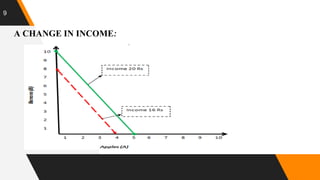
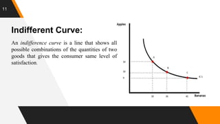
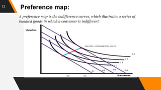
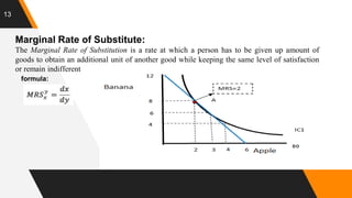
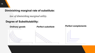
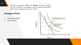
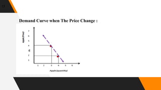
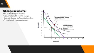
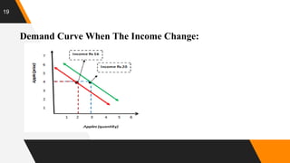
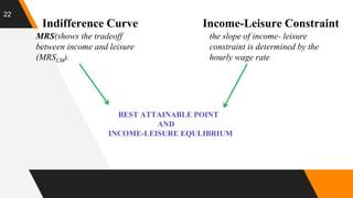
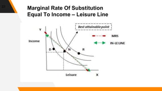
This document discusses household consumption possibilities, preferences, and choices. It covers budget lines, indifference curves, and how they are used to predict consumer behavior. It also discusses work-leisure choices. Specifically, it defines budget lines and how they are determined by income and prices. It introduces indifference curves and preference maps. It explains how marginal rates of substitution are used, and the law of diminishing marginal rate of substitution. It discusses how changes in prices and income affect consumer choice and demand curves. Finally, it covers the income-leisure constraint and how wage rates determine the slope of the constraint line, affecting the labor supply curve.

1. Possibility,Preference
And Choices

2. INTRODUCTION:
2
1. Household consumption possibilities , preferences and
choices.
a. Budget line.
b. Indifference curve.
c. Predicting consumer behavior.
d. Work-leisure choices.

3. 1.
Budget line:
budget line shows the combination of two
products that a consumer can afford to buy with
a given income
Two things determine budget line:
1. Income of household.
2. Price of goods.
3

4. 4
Combination of
Apples and
Bananas
Apples(A) 4
each
Bananas(B) 2
each
Money spent
=Income (Rs.)
E 5 0 (5*4)+(0*2)=2
0
F 4 2 (4*4)+(2*2)=2
0
G 3 4 (3*4)+(4*2)=2
0
H 2 6 (2*4)+(6*2)=2
0
I 1 8 (1*4)+(8*2)=2
0
J 0 10 (0*4)+(10*2)=
20
Hafsa Kaleem Schedule of
Budget Line:
EXAMPLE:

5. “DIVISIBLE GOODS:
Some goods that can be bought in any quantity desired are divisible goods.
INDIVISIBLE GOODS:
Those goods which can be sold in discrete quantities are indivisible goods.

6. 6
BUDGET EQUATION:
Budget line can be described by the budget equation. The budget equation starts by the fact
that.
Expenditure = Income
Expenditure = ( Price of banana*Quantity of banana ) + ( Price of apple*Quantity of apple )
(PB)(QB) + (PA)(QA) = M
2QB + 4QA = 20
QB + 2QA = 10
Affordable Quantities Unaffordable Quantities
Point inside the boundary Point outside the boundary

7. 7
REAL INCOME: (Purchasing power)
A real income is a income in terms of quantity of goods that a household can afford to buy.
(M)Total income
(P)Price of goods Real Income M/P Apple or P Banana
RELATIVE PRICE:
Relative price is the price of one good divided by the price of another good.
Price of Apple( PA)
Price of banana( PB)
Relative price PA/PB

8. 8
A CHANGE IN PRICE:

9. 9
A CHANGE IN INCOME:

10. Preferences And
Indifference Curve:
2.

11. 11
Indifferent Curve:
An indifference curve is a line that shows all
possible combinations of the quantities of two
goods that gives the consumer same level of
satisfaction.

12. 12
Preference map:
A preference map is the indifference curves, which illustrates a series of
bundled goods in which a consumer is indifferent.

13. 13
Marginal Rate of Substitute:
The Marginal Rate of Substitution is a rate at which a person has to be given up amount of
goods to obtain an additional unit of another good while keeping the same level of satisfaction
or remain indifferent
formula:

14. 14
Diminishing marginal rate of substitute:
law of diminishing marginal utility.
Degree of Substitutability:
Ordinary goods Perfect substitute Perfect complements

15. Predicting
Consumer Choice
Consumer choice and maximum utility can be
predicted through utilizing these major economic
tools;
•Budget line
•Indifference curve
•Marginal substitute rate(MRS)
3.

16. 16
Changes in two factors; Price and Income can bring a change
into the commodity consumption and the quantity demanded
(Qd) means a change in consumer’s choice.
Change in Price:
1. Substitution effect
2. Income effect

17. 17
Demand Curve when The Price Change :

18. 18
Change in Income:
Due to the change in income:
•Highest attainable point is change.
•Generate income and substitution effect.
•Price of goods remains constant.

19. 19
Demand Curve When The Income Change:

20. Work Leisure
Choices
4.

21. 21
24 HOURS
LEISURE WORK
Non-paid
hours
paid hours

22. 22
Indifference Curve Income-Leisure Constraint
MRS(shows the tradeoff
between income and leisure
(MRSLM).
the slope of income- leisure
constraint is determined by the
hourly wage rate
BEST ATTAINABLE POINT
AND
INCOME-LEISURE EQULIBRIUM

23. 23
Marginal Rate Of Substitution
Equal To Income – Leisure Line

24. 24
Wage offer Curve and Labor supply Curve:
Changes in the wage rate can produce
Increase in
labor supply
Decrease in
labor supply
no change
labor supply
Change is because of
substitution & income effect

25. 25
Wage offer Curve and Labor supply Curve:
Hafsa Kaleem Labor supply curve

26. 26
SHIFT IN LABOUR SUPPLY:
1. Change in preference
2. Change in income (that can be labor income or non-
labor income)
3. Change in climate
4. Change in population.

27. 27
Labor Supply over the Business Cycle:
Added worker effect
OR
Discourage labor effect.
RECESSION
(rises during recessions and falls
during expansions)
(falls during recessions and increases
during expansions)

28. 28
The Economic Concept of Work –Leisure Choice in
Real World:
Pakistan
According to the law, the normal working hours per day are
8-9 hours and these should not be more than 48 hours per
week.
India
Working Hours in India:) cannot work for more than 48
hours in a week and not more than 9 hours in a day.
South Africa the maximum normal working time allowed is 45 hours
weekly. This is nine hours per day (excluding a lunch
break).

29. “THANK YOU&
ANY QUESTIONS?