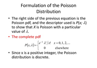
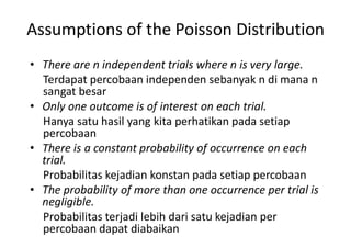
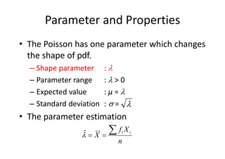
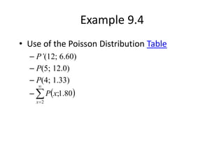
BASICS OF THE POISSON
DISTRIBUTION
Formulation of the Poisson
Distribution
• If you look closely at a photograph in a
newspaper, you see that the image is
composed of a large number of dots arranged
in rows and columns.
• Each dot is printed larger for a dark area and
smaller for light areas.
• Any one of the dots is printed incorrectly if it
is too light, too dark, missing, or misplaced.
Formulation of the Poisson
Distribution
• Define:
– h = area represented by one dot; h > 0 but very small
– µ = constant representing average number of times dot is
printed incorrectly in h; µ > 0
– H = total area, divided into n equal areas, each containing
a dot
• The area h = H/n gets smaller and smaller as n
becomes countably infinite (n = 0, 1, 2, …, no upper
limit).
Formulation of the Poisson
Distribution
• We postulate that the probability of an
incorrectly printed dot is proportional to the
size of h; that is, as the area h increases, the
probability of an incorrect dot increases.
Therefore
– µh = probability of one incorrectly printed dot in h
– 1 - µh = probability of a correctly printed dot in h
• Since µh + (1 - µh) = 1, there is no chance of
more than one mistake in any h.
Formulation of the Poisson
Distribution
• The small value µh is called a rare event
probability, and it is used to derive the
Poisson pdf from the binomial by substituting
µh for p:
• Take the limit as n  , as p  0, and with np
constant (call its value ), and the Poisson pdf
results:
n
H
h
p 
 

 
!
,
;
limit
0
x
e
p
n
x
b
x
np
p
n









Formulation of the Poisson
Distribution
• The right side of the previous equation is the
Poisson pdf, and the descriptor used is P(x; )
to show that X is Poisson with a particular
value of .
• The complete pdf
• Since x is a positive integer, the Poisson
distribution is discrete.
 


 


elsewhere
0
...
2,
1,
0,
!
,
x
x
e
x
P
x



Assumptions of the Poisson Distribution
• There are n independent trials where n is very large.
Terdapat percobaan independen sebanyak n di mana n
sangat besar
• Only one outcome is of interest on each trial.
Hanya satu hasil yang kita perhatikan pada setiap
percobaan
• There is a constant probability of occurrence on each
trial.
Probabilitas kejadian konstan pada setiap percobaan
• The probability of more than one occurrence per trial is
negligible.
Probabilitas terjadi lebih dari satu kejadian per
percobaan dapat diabaikan
Definition of the Poisson Distribution
The Poisson is a discrete distribution which
estimates the probability that a specified
outcome will occur exactly x times in a
standardized unit when the average rate of
occurrence per unit is a constant .
Parameter and Properties
• The Poisson has one parameter which changes
the shape of pdf.
– Shape parameter : 
– Parameter range :  > 0
– Expected value : µ = 
– Standard deviation :  =
• The parameter estimation

n
X
f
X i
i



̂
Example 9.3
Dolly and Darrel are engineers with a government-
sponsored safety agency. They have determined the
number of serious accident each month at the
construction sites of new government office buildings to
be Poisson-distributed.
a. Based on the data below, they predict a good change
of one serious accident each month. Are they correct?
b. What are the 1 limits above and below the mean of
this data?
5
4
3
2
1
0
Accidents
per month
0
1
2
8
12
27
Frequency
Example 9.4
• Use of the Poisson Distribution Table
– P’(12; 6.60)
– P(5; 12.0)
– P(4; 1.33)
–  


2
80
.
1
;
x
x
P
Solving Problems Using the Poisson
• Check assumptions
• Determine the variable and value of the
parameter.
• Obtain a single Poisson probability.
• Obtain the sum of several Poisson probability
values.
• Determine µ and  for the Poisson.
• Plot the pdf or cdf.
Example 9.5
An ME is studying the defect pattern in cold-rolled
steel. The engineer inspects 10-m sections to
determine the number of defects D. The results for 50
sections are:
Number of
sections
Defects per
section D
35
8
3
2
1
1
50
0
1
2
3
4
6
a. Determine the probability of
being on or above the
specification limit of three
defects per section.
b. Compute the 3 limits.
Example 9.6
Problems
• 9.6
• 9.10 (c)
• 9.13
• 9.18

Poisson Distribution Poisson Distribution

  • 1.
    BASICS OF THEPOISSON DISTRIBUTION
  • 2.
    Formulation of thePoisson Distribution • If you look closely at a photograph in a newspaper, you see that the image is composed of a large number of dots arranged in rows and columns. • Each dot is printed larger for a dark area and smaller for light areas. • Any one of the dots is printed incorrectly if it is too light, too dark, missing, or misplaced.
  • 3.
    Formulation of thePoisson Distribution • Define: – h = area represented by one dot; h > 0 but very small – µ = constant representing average number of times dot is printed incorrectly in h; µ > 0 – H = total area, divided into n equal areas, each containing a dot • The area h = H/n gets smaller and smaller as n becomes countably infinite (n = 0, 1, 2, …, no upper limit).
  • 4.
    Formulation of thePoisson Distribution • We postulate that the probability of an incorrectly printed dot is proportional to the size of h; that is, as the area h increases, the probability of an incorrect dot increases. Therefore – µh = probability of one incorrectly printed dot in h – 1 - µh = probability of a correctly printed dot in h • Since µh + (1 - µh) = 1, there is no chance of more than one mistake in any h.
  • 5.
    Formulation of thePoisson Distribution • The small value µh is called a rare event probability, and it is used to derive the Poisson pdf from the binomial by substituting µh for p: • Take the limit as n  , as p  0, and with np constant (call its value ), and the Poisson pdf results: n H h p       ! , ; limit 0 x e p n x b x np p n         
  • 6.
    Formulation of thePoisson Distribution • The right side of the previous equation is the Poisson pdf, and the descriptor used is P(x; ) to show that X is Poisson with a particular value of . • The complete pdf • Since x is a positive integer, the Poisson distribution is discrete.         elsewhere 0 ... 2, 1, 0, ! , x x e x P x   
  • 7.
    Assumptions of thePoisson Distribution • There are n independent trials where n is very large. Terdapat percobaan independen sebanyak n di mana n sangat besar • Only one outcome is of interest on each trial. Hanya satu hasil yang kita perhatikan pada setiap percobaan • There is a constant probability of occurrence on each trial. Probabilitas kejadian konstan pada setiap percobaan • The probability of more than one occurrence per trial is negligible. Probabilitas terjadi lebih dari satu kejadian per percobaan dapat diabaikan
  • 8.
    Definition of thePoisson Distribution The Poisson is a discrete distribution which estimates the probability that a specified outcome will occur exactly x times in a standardized unit when the average rate of occurrence per unit is a constant .
  • 9.
    Parameter and Properties •The Poisson has one parameter which changes the shape of pdf. – Shape parameter :  – Parameter range :  > 0 – Expected value : µ =  – Standard deviation :  = • The parameter estimation  n X f X i i    ̂
  • 10.
    Example 9.3 Dolly andDarrel are engineers with a government- sponsored safety agency. They have determined the number of serious accident each month at the construction sites of new government office buildings to be Poisson-distributed. a. Based on the data below, they predict a good change of one serious accident each month. Are they correct? b. What are the 1 limits above and below the mean of this data? 5 4 3 2 1 0 Accidents per month 0 1 2 8 12 27 Frequency
  • 11.
    Example 9.4 • Useof the Poisson Distribution Table – P’(12; 6.60) – P(5; 12.0) – P(4; 1.33) –     2 80 . 1 ; x x P
  • 12.
    Solving Problems Usingthe Poisson • Check assumptions • Determine the variable and value of the parameter. • Obtain a single Poisson probability. • Obtain the sum of several Poisson probability values. • Determine µ and  for the Poisson. • Plot the pdf or cdf.
  • 13.
    Example 9.5 An MEis studying the defect pattern in cold-rolled steel. The engineer inspects 10-m sections to determine the number of defects D. The results for 50 sections are: Number of sections Defects per section D 35 8 3 2 1 1 50 0 1 2 3 4 6 a. Determine the probability of being on or above the specification limit of three defects per section. b. Compute the 3 limits.
  • 14.
  • 15.
    Problems • 9.6 • 9.10(c) • 9.13 • 9.18