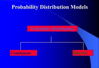
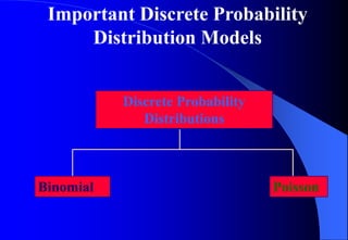
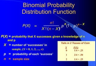
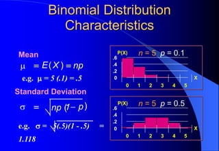
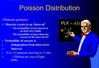
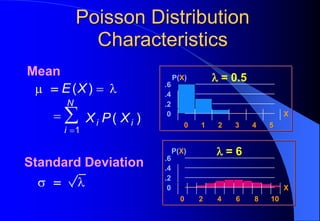
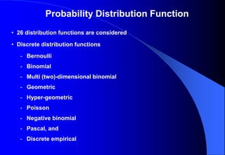
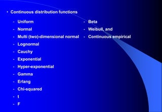
NAME
STREAM
COLL ROLL NO.
SUBJECT
SUBJECT CODE
SESSION
YEAR
: ROHIT BOURI
: MECHANICAL ENGINEERING
: 237123063
: MATHEMATICS III
: BS-M301
: 2023-24
: 2ND YEAR ( 3RD SEM)
POWERPOINT PRESENTATI ON DISTRIBUTION FUNCTION
BENGAL COLLEGE OF
ENGINEERING AND TECHNOLOGY
Probability Distribution Models
Probability Distributions
Continuous Discrete
Important Discrete Probability
Distribution Models
Discrete Probability
Distributions
Binomial Poisson
Binomial Distributions
⚫ ‘N’ identical trials
– E.G. 15 tosses of a coin, 10 light bulbs taken from a
warehouse
⚫ 2 mutually exclusive outcomes on each trial
– E.G. Heads or tails in each toss of a coin, defective or
not defective light bulbs
⚫
Binomial Distributions
⚫
• Constant Probability for each Trial
• e.g. Probability of getting a tail is the same each
time we toss the coin and each light bulb has the
same probability of being defective
• 2 Sampling Methods:
• Infinite Population Without Replacement
• Finite Population With Replacement
• Trials are Independent:
• The Outcome of One Trial Does Not Affect the
Outcome of Another
Binomial Probability
Distribution Function
P(X) = probability that X successes given a knowledge of n
and p
X = number of ‘successes’ in
sample, (X = 0, 1, 2, ..., n)
p = probability of each ‘success’
n = sample size
P(X)
n
X ! n X
p p
X n X
!
( )!
( )
=
−
−
−
1
Tails in 2 Tosses of Coin
X P(X)
0 1/4 = .25
1 2/4 = .50
2 1/4 = .25
Binomial Distribution
Characteristics
n = 5 p = 0.1
n = 5 p = 0.5
Mean
Standard Deviation


E X np
np p
= =
= −
( )
( )
0
.2
.4
.6
0 1 2 3 4 5
X
P(X)
.2
.4
.6
0 1 2 3 4 5
X
P(X)
e.g.  = 5 (.1) = .5
e.g.  = 5(.5)(1 - .5) =
1.118
0
Poisson Distribution
⚫Poisson process:
⚫ Discrete events in an ‘interval’
– The probability of one success in
an interval is stable
– The probability of more than one
success in this interval is 0
⚫ Probability of success is
⚫ Independent from interval to
⚫ Interval
⚫ E.G. # Customers arriving in 15 min
⚫ # Defects per case of light
bulbs
P X x
x
x
( |
!
= 


e-
Poisson Distribution Function
P(X ) = probability of X successes given 
 = expected (mean) number of ‘successes’
e = 2.71828 (base of natural logs)
X = number of ‘successes’ per unit
P X
X
X
( )
!
= 
−
e
e.g. Find the probability of 4
customers arriving in 3 minutes
when the mean is 3.6.
P(X) = e
-3.6
3.6
4!
4
= .1912
Poisson Distribution
Characteristics
 = 0.5
 = 6
Mean
Standard Deviation
 
 
i
i
N
i
E X
X P X
= =
=
=
=

( )
( )
1
0
.2
.4
.6
0 1 2 3 4 5
X
P(X)
0
.2
.4
.6
0 2 4 6 8 10
X
P(X)
Probability Distribution Function
• 26 distribution functions are considered
• Discrete distribution functions
- Bernoulli
- Binomial
- Multi (two)-dimensional binomial
- Geometric
- Hyper-geometric
- Poisson
- Negative binomial
- Pascal, and
- Discrete empirical
• Continuous distribution functions
- Uniform
- Normal
- Multi (two)-dimensional normal
- Lognormal
- Cauchy
- Exponential
- Hyper-exponential
- Gamma
- Erlang
- Chi-squared
- t
- F
- Beta
- Weibull, and
- Continuous empirical
p Gamma
Exponential
0 x
The Normal Distribution
⚫ ‘Bell Shaped’
⚫ Symmetrical
⚫ Mean, Median and
⚫ Mode are Equal
⚫ ‘Middle Spread’
⚫ Equals 1.33 
⚫ Random Variable has
⚫ Infinite Range
Mean
Median
Mode
X
f(X)

Varying the Parameters  and , we obtain
Different Normal Distributions.
There are an
Infinite
Number
Many Normal Distributions
Poisson
p
x
0
Poisson Distribution Function
P(X ) = probability of X successes given 
 = expected (mean) number of ‘successes’
e = 2.71828 (base of natural logs)
X = number of ‘successes’ per unit
P X
X
X
( )
!
= 
−
e
e.g. Find the probability of 4
customers arriving in 3 minutes
when the mean is 3.6.
P(X) = e
-3.6
3.6
4!
4
= .1912
Uniform
p
0 a b x
EXAMPLE OF SOFTWARES FOR SIMULATION
1. Statfit
2. PowerSim
3. VenSim
4. Stella
5. IThink
The Normal Distribution
⚫ ‘Bell Shaped’
⚫ Symmetrical
⚫ Mean, Median and
⚫ Mode are Equal
⚫ ‘Middle Spread’
⚫ Equals 1.33 
⚫ Random Variable has
⚫ Infinite Range
Mean
Median
Mode
X
f(X)

Thank You

MATH.pdf

  • 1.
    NAME STREAM COLL ROLL NO. SUBJECT SUBJECTCODE SESSION YEAR : ROHIT BOURI : MECHANICAL ENGINEERING : 237123063 : MATHEMATICS III : BS-M301 : 2023-24 : 2ND YEAR ( 3RD SEM) POWERPOINT PRESENTATI ON DISTRIBUTION FUNCTION BENGAL COLLEGE OF ENGINEERING AND TECHNOLOGY
  • 2.
    Probability Distribution Models ProbabilityDistributions Continuous Discrete
  • 3.
    Important Discrete Probability DistributionModels Discrete Probability Distributions Binomial Poisson
  • 4.
    Binomial Distributions ⚫ ‘N’identical trials – E.G. 15 tosses of a coin, 10 light bulbs taken from a warehouse ⚫ 2 mutually exclusive outcomes on each trial – E.G. Heads or tails in each toss of a coin, defective or not defective light bulbs ⚫
  • 5.
    Binomial Distributions ⚫ • ConstantProbability for each Trial • e.g. Probability of getting a tail is the same each time we toss the coin and each light bulb has the same probability of being defective • 2 Sampling Methods: • Infinite Population Without Replacement • Finite Population With Replacement • Trials are Independent: • The Outcome of One Trial Does Not Affect the Outcome of Another
  • 6.
    Binomial Probability Distribution Function P(X)= probability that X successes given a knowledge of n and p X = number of ‘successes’ in sample, (X = 0, 1, 2, ..., n) p = probability of each ‘success’ n = sample size P(X) n X ! n X p p X n X ! ( )! ( ) = − − − 1 Tails in 2 Tosses of Coin X P(X) 0 1/4 = .25 1 2/4 = .50 2 1/4 = .25
  • 7.
    Binomial Distribution Characteristics n =5 p = 0.1 n = 5 p = 0.5 Mean Standard Deviation   E X np np p = = = − ( ) ( ) 0 .2 .4 .6 0 1 2 3 4 5 X P(X) .2 .4 .6 0 1 2 3 4 5 X P(X) e.g.  = 5 (.1) = .5 e.g.  = 5(.5)(1 - .5) = 1.118 0
  • 8.
    Poisson Distribution ⚫Poisson process: ⚫Discrete events in an ‘interval’ – The probability of one success in an interval is stable – The probability of more than one success in this interval is 0 ⚫ Probability of success is ⚫ Independent from interval to ⚫ Interval ⚫ E.G. # Customers arriving in 15 min ⚫ # Defects per case of light bulbs P X x x x ( | ! =    e-
  • 9.
    Poisson Distribution Function P(X) = probability of X successes given   = expected (mean) number of ‘successes’ e = 2.71828 (base of natural logs) X = number of ‘successes’ per unit P X X X ( ) ! =  − e e.g. Find the probability of 4 customers arriving in 3 minutes when the mean is 3.6. P(X) = e -3.6 3.6 4! 4 = .1912
  • 10.
    Poisson Distribution Characteristics  =0.5  = 6 Mean Standard Deviation     i i N i E X X P X = = = = =  ( ) ( ) 1 0 .2 .4 .6 0 1 2 3 4 5 X P(X) 0 .2 .4 .6 0 2 4 6 8 10 X P(X)
  • 11.
    Probability Distribution Function •26 distribution functions are considered • Discrete distribution functions - Bernoulli - Binomial - Multi (two)-dimensional binomial - Geometric - Hyper-geometric - Poisson - Negative binomial - Pascal, and - Discrete empirical
  • 12.
    • Continuous distributionfunctions - Uniform - Normal - Multi (two)-dimensional normal - Lognormal - Cauchy - Exponential - Hyper-exponential - Gamma - Erlang - Chi-squared - t - F - Beta - Weibull, and - Continuous empirical
  • 13.
  • 14.
    The Normal Distribution ⚫‘Bell Shaped’ ⚫ Symmetrical ⚫ Mean, Median and ⚫ Mode are Equal ⚫ ‘Middle Spread’ ⚫ Equals 1.33  ⚫ Random Variable has ⚫ Infinite Range Mean Median Mode X f(X) 
  • 15.
    Varying the Parameters and , we obtain Different Normal Distributions. There are an Infinite Number Many Normal Distributions
  • 16.
  • 17.
    Poisson Distribution Function P(X) = probability of X successes given   = expected (mean) number of ‘successes’ e = 2.71828 (base of natural logs) X = number of ‘successes’ per unit P X X X ( ) ! =  − e e.g. Find the probability of 4 customers arriving in 3 minutes when the mean is 3.6. P(X) = e -3.6 3.6 4! 4 = .1912
  • 18.
  • 19.
    EXAMPLE OF SOFTWARESFOR SIMULATION 1. Statfit 2. PowerSim 3. VenSim 4. Stella 5. IThink
  • 20.
    The Normal Distribution ⚫‘Bell Shaped’ ⚫ Symmetrical ⚫ Mean, Median and ⚫ Mode are Equal ⚫ ‘Middle Spread’ ⚫ Equals 1.33  ⚫ Random Variable has ⚫ Infinite Range Mean Median Mode X f(X) 
  • 21.