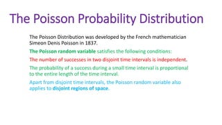
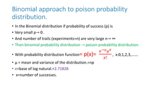
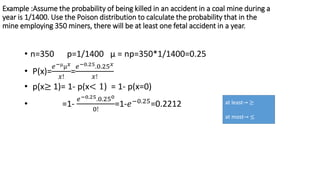
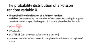
The Poisson distribution describes the number of events occurring in a fixed interval of time or space if these events occur with a known average rate and independently of the time since the last event. The document provides details about the Poisson distribution, including its properties and applications. It also provides an example derivation of the Poisson distribution as an approximation to the binomial distribution when the probability of success is very small and the number of trials is very large.

1. The Poisson Probability Distribution
The Poisson Distribution was developed by the French mathematician
Simeon Denis Poisson in 1837.
The Poisson random variable satisfies the following conditions:
The number of successes in two disjoint time intervals is independent.
The probability of a success during a small time interval is proportional
to the entire length of the time interval.
Apart from disjoint time intervals, the Poisson random variable also
applies to disjoint regions of space.

2. Binomial approach to poison probability
distribution.
• In the Binomial distribution if probability of success (p) is
• Very small p→ 0.
• And number of trails (experiments=n) are very large n→ ∞
• Then binomial probability distribution → poison probability distribution.
• With probability distribution function= p(x)=
𝑒−µµ𝑥
𝑥!
, x:0,1,2,3,…….
• µ = mean and variance of the distribution.=np
• e=base of log natural.=2.71828
• x=number of successes.

3. Example: In the past experience in the production of a certain component has shown
the production of defectives is 0.03. component leaves the factory in
boxes of 500.
what is the probability that
1. a box contains 3 or more defectives.
2. two successive boxes contains 6 or more defectives intem.
• P=0.03 n=500
• P(x≥ 3)=?
• µ =np=500*0.03=15
• P(x)=
𝒆−µµ𝒙
𝒙!
=
𝑒−15.15𝑥
𝑥!
• P(x≥ 3)=1- p(x< 3)= 1 – [p(x=0)+p(x=1)+p(x=2)]
• =1- [
𝑒−15.150
0!
+
𝑒−15.151
1!
+
𝑒−15.152
2!
]
• =1-[𝑒−15+𝑒−15. 151+
𝑒−15.152
2
]
• =1-0.0000393=0.99997
• 2. p=0.03 in two boxes number of items= n=500+500=1000

4. N=1000 p=0.03 µ =np=1000*0.03=30
• P(x)=
𝒆−µµ𝒙
𝒙!
=
𝑒−30∗30𝑥
𝑥!
• P(x≥ 6)= 1- p(x< 6)
• =1-[p(x=0)+p(x=1)+p(x=2)+p(x=3)+p(x=4)+p(x=4)+p(x=5)]
• =1-[
𝑒−30∗300
0!
+
𝑒−30∗301
1!
+
𝑒−30∗302
2!
+
𝑒−30∗303
3!
+
𝑒−30∗304
4!
+
𝑒−30∗305
5!
]
• = 1-0.0000000256=0.99999999

5. Example :Assume the probability of being killed in an accident in a coal mine during a
year is 1/1400. Use the Poison distribution to calculate the probability that in the
mine employing 350 miners, there will be at least one fetal accident in a year.
• n=350 p=1/1400 µ = np=350*1/1400=0.25
• P(x)=
𝑒−µµ𝑥
𝑥!
=
𝑒−0.25.0.25𝑥
𝑥!
• p(x≥ 1)= 1- p(x< 1) = 1- p(x=0)
• =1-
𝑒−0.25.0.250
0!
=1-𝑒−0.25
=0.2212 at least→ ≥
at most→ ≤

6. Area of application
• Applications
• the number of deaths by horse kicking in the Prussian army (first application)
• birth defects and genetic mutations
• rare diseases (like Leukemia, but not AIDS because it is infectious and so not
independent) - especially in legal cases
• car accidents
• traffic flow and ideal gap distance
• number of typing errors on a page
• hairs found in McDonald's hamburgers
• spread of an endangered animal in Africa
• failure of a machine in one month

7. The probability distribution of a Poisson
random variable X.
• The probability distribution of a Poisson random
variable X representing the number of successes occurring in a given
time interval or a specified region of space is given by the formula:
• p(x)=
𝑒−µµ𝑥
𝑥!
• x=0,1,2,3…
• e=2.71828 (but use your calculator's e button)
• μ= mean number of successes in the given time interval or region of
space

8. Derivation of poison probability distribution:
approximation to binomial distribution.
• In the binomial distribution b(x:n,p)=𝐶𝑥
𝑛
𝑝𝑥
𝑞𝑛−𝑥
• if p→ 0 and n → ∞ and the product np remains the constant then binomial → poison
distribution
• b(x:n,p)=𝐶𝑥
𝑛
𝑝𝑥
𝑞𝑛−𝑥
x:0,1,2,……..,n
• =
𝑛!
𝑥!(𝑛−𝑥)!
𝑝𝑥𝑞𝑛−𝑥
• =
n(n−1)(n−2)(n−3)(n−4)………..(n−(x−1))(n−x)!
𝑥!(𝑛−𝑥)!
𝑝𝑥
𝑞𝑛−𝑥
• =
n(n−1)(n−2)(n−3)(n−4)………..(n−x+1)
𝑥!
𝑝𝑥
𝑞𝑛−𝑥
• as np=µ , p=
µ
𝑛
q=1-p= 1-
µ
𝑛
• Putting the values of p and q.
• =
n(n−1)(n−2)(n−3)(n−4)………..(n−x+1)
𝑥!
(
µ
𝑛
)𝑥(1−
µ
𝑛
)𝑛−𝑥

9. • =
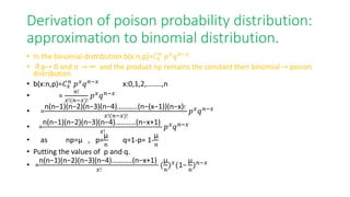
n(n−1)(n−2)(n−3)(n−4)………..(n−x+1)
𝑥!
(
µ
𝑛
)𝑥(1−
µ
𝑛
)𝑛−𝑥
• =
µ𝑥
𝑥!
n(n−1)(n−2)(n−3)(n−4)………..(n−x+1)
𝑛𝑥 (1−
µ
𝑛
)𝑛−𝑥
• =
µ𝑥
𝑥!
n(n−1)(n−2)(n−3)(n−4)………..[n−(x−1)]
𝑛𝑥 (1−
µ
𝑛
)𝑛(1−
µ
𝑛
)−𝑥
•
µ𝑥
𝑥!
1 −
1
n
1 −
2
n
1 −
3
n
… . . (1 −
𝑥−1
𝑛
)(1−
µ
𝑛
)𝑛(1−
µ
𝑛
)−𝑥
• if p→ 0 and n → ∞

10. •
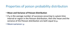
µ𝑥
𝑥!
1.1.1.1……1. lim
𝑛→∞
1 −
µ
𝑛
𝑛
lim
𝑛→∞
1 −
µ
𝑛
−𝑥
• as 1/∞=0
•
µ𝑥
𝑥!
lim
𝑛→∞
1 −
µ
𝑛
𝑛
• Let
𝑛
µ
=k then n= µk
•
µ𝑥
𝑥!
lim
𝑘→∞
1 −
1
𝑘
µk
•
•
µ𝑥
𝑥!
[ lim
𝑘→∞
1 −
1
𝑘
−𝑘
]
−µ
=
µ𝑥
𝑥!
[e] −µ ∵ lim
𝑘→∞
1 −
1
𝑘
−𝑘
= e
• P(x: µ) =
e −µµ
𝑥
𝑥!
, x:0,1,2,……..n

11. Properties of poison probability distribution
• Mean and Variance of Poisson Distribution
• If μ is the average number of successes occurring in a given time
interval or region in the Poisson distribution, then the mean and the
variance of the Poisson distribution are both equal to μ.
• Mean=variance= μ

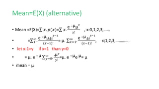
12. Mean
• Mean =E(X)= 𝑥. 𝑝(𝑥)= 𝑥.
e −µµ
𝑥
𝑥!
, x:0,1,2,3,……
• = 0. e −µµ
0
+1.
e −µµ
1
1!
+2.
e −µµ
2
2!
+3
e −µµ
3
3!
+4
e −µµ
4
4!
+……..
• = e −µµ
1
+
e −µµ
2
1!
+
e −µµ
3
2!
+
e −µµ
4
3!
+……..
• =e −µµ
1
[1+
µ1
1!
+
µ2
2!
+
µ3
3!
+……..]
• =e −µµ
1
[e µ]
• mean = µ

13. Mean=E(X) (alternative)
• Mean =E(X)= 𝑥. 𝑝(𝑥)= 𝑥.
e −µµ
𝑥
𝑥!
, x:0,1,2,3,……
• = 1
∞
.
e −µµ.µ
𝑥−1
(𝑥−1)!
= µ. 𝑥=1
∞
.
e −µ.µ
𝑥−1
(𝑥−1)!
, x;1,2,3,………….
• let x-1=y if x=1 than y=0
• = µ. e −µ
𝑦=0
∞
.
.µ𝑦
𝑦!
=µ. e −µe µ= µ
• mean = µ

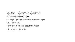
14. Variance =E[𝑋2
]-[𝐸(𝑋)]2
-----------1
• 𝑋2=x(x-1)+x
• E(𝑋2)=E[x(x-1)]+E(x)
• = 𝑥 𝑥 − 1 . 𝑝 𝑥 + µ= 𝑥=0
∞
𝑥 𝑥 − 1 .
e −µµ
𝑥
𝑥!
+ µ
• = 𝑥=0
∞
𝑥(𝑥 − 1).
µ2
e −µ µ
𝑥−2
𝑥(𝑥−1)(𝑥−2)!
+ µ
• =µ2e −µ
𝑥=2
∞
.
µ𝑥−2
(𝑥−2)!
+ µ
• Let x-2=y , x=2 then y=0

15. • E(𝑋2
)=µ2
e −µ
𝑦=0
∞
.
µ𝑦
𝑦!
+ µ
• =µ2e −µe µ+ µ
• E(𝑋2
)=µ2
+ µ … . …….2
• Variance =E[𝑋2]-[𝐸(𝑋)]2----------1
• putting the value of eq. 2 in eq. 1
• Variance =µ2
+ µ − [µ]2
= µ
• Variance = µ
• µ2
/
= E(𝑋2
) µ3
/
= E(𝑋3
)=?, µ4
/
= E(𝑋4
)=?

16. • µ2
/
= E(𝑋2 ) µ3
/
= E(𝑋3)=?, µ4
/
= E(𝑋4)=?
• 𝑋3=x(x-1)(x-2)+3x(x-1)+x
• 𝑋4 =x(x-1)(x-2)(x-3)+6x(x-1)(x-2)+7x(x-1)+x
• 𝛽1 and 𝛽2
• first four moments about the mean
• µ1 , µ2 , µ3 , µ4

17. Reproductive productive property of poison
distribution.
• If two independent variables X and Y have the poison distribution with
parameters µ and v respectively, then their sum X+Y has poison
distribution with parameter µ + v .
• Proof: Here X is p(x: µ) and Y is p(y: v) and we want to find that p(x+y=k),
k:0,1,2,3,……..
• p(X=x)=
e −µµ
𝑥
𝑥!
.
• p(Y=y)=
e −𝑣
𝑣𝑦
𝑦!
• K=0 , p(x+y=0)=p(x=0)p(y=0)=
e −µµ
0
0!
.
e −𝑣
𝑣0
0!
=e −µe −𝑣
=e −(µ+v)

18. • k=1, p(x+y=1)=p(x=1)p(y=0)+p(x=0)p(y=1)
• =
e −µµ
1
1!
.
e −𝑣
𝑣0
0!
+
e −µµ
0
0!
.
e −𝑣
𝑣1
1!
=
e −(µ+v)(µ+v)
1
1!
• K=2
• p(x+y=2) = p(x=2)p(y=0)+p(x=1)p(y=1)+ p(x=0)p(y=2) =
e −(µ+v)(µ+v)
2
2!
• =
e −µµ
2
2!
.
e −𝑣
𝑣0
0!
+
e −µµ
1
1!
.
e −𝑣
𝑣1
1!
+
e −µµ
0
0!
.
e −𝑣
𝑣2
2!
=
e −(µ+v)(µ+v)
2
2!
• =
e −(µ+v)
2!
{µ2
+ 2 µv+ 𝑣2
}=
e −(µ+v)(µ+v)
2
2!

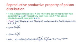
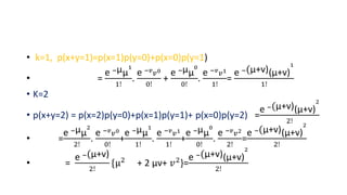
19. • k=k
• P(x+y=k)
• = p(x=0)p(y=k)+p(x=1)p(y=k-1)+ p(x=k)p(y=0)
• + p(x=k-1)p(y=1)……..p(x=i)p(y=k-i)
• =
e −µµ
0
0!
.
e −𝑣
𝑣𝑘
𝑘!
+
e −µµ
1
1!
.
e −𝑣
𝑣𝑘−1
(𝑘−1)!
+……….+
e −µµ
𝑘
𝑘!
.
e −𝑣
𝑣0
0!
• =e −(µ+v)[.
𝑣𝑘
𝑘!
+
µ1
1!
.
𝑣𝑘−1
(𝑘−1)!
+……….+
µ𝑘
𝑘!
.]=
• P(x+y=k)=
e −(µ+v)[µ+v]
𝑘
𝑘!

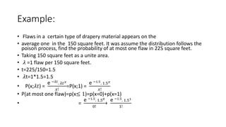
20. Example :
• A secretary makes 2 errors per page on the average. What is the
probability that on the next page she will make: i) 4 0r more errors ii)
no error.
• P(x=µ)=
e −µµ
𝑥
𝑥!
=
e −2
2𝑥
𝑥!
• i) p(x≥ 4)=1-p(x<4)= 1-[ p(x=0)+p(x=1)+p(x=2)+p(x=3)]
• Ii) p(x=0)

21. X=no. of deaths= 0 1 2 3 4 5
f= frequencies= 109 65 22 3 1 0/200
fit the poison distribution.
• Mean = µ =
𝑓𝑥
𝑓
=0.61
• p(X=x)=
e −µµ
𝑥
𝑥!
=
e −0.61
0.61𝑥
𝑥!
• x f fx p(X=x) expected frequencies=𝑓𝑒=N*p(x)
• 0 0.5434 200* 0.5434=108.68
• 1 0.3314 66.28
• 2 0.1011 20.22
• 3 0.0206 4.12
• 4 0.00313 0.626
• 5 0.00038 0

22. Poison process.
• The probability of an event occurs in a very short interval of time t,
• is proportion to the length of time interval. Distribution for
• the process is as follows:
• P(x;𝜆𝑡) =
e −𝜆𝑡
. (𝜆𝑡)𝑥
𝑥!
• 𝜆 = average no. occurrence per unit time.
• t=time interval
• X= number of occurrences in t unites of time.

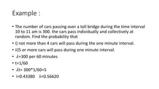
23. Example :
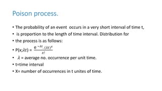
• Telephone calls are being placed through certain exchange at random
time on the average 4 per minute. Assume that a poison process ,find
the probability that in the 15 seconds there are 3 are more calls.
• 𝜆 =4 calls per minute
• t= 15/60=1/4
• 𝜆t=4*1/4=1
• p( x≥ 3) = 1 – p(x< 3)=1-[p(x=0)+p(x=1)+p(x=2)]
• P(x;𝜆𝑡) =
e −𝜆𝑡
. (𝜆𝑡)𝑥
𝑥!
=P(x;1) =
e −1
. 1𝑥
𝑥!

24. Example:
• Flaws in a certain type of drapery material appears on the
• average one in the 150 square feet. It was assume the distribution follows the
poison process, find the probability of at most one flaw in 225 square feet.
• Taking 150 square feet as a unite area.
• 𝜆 =1 flaw per 150 square feet.
• t=225/150=1.5
• 𝜆t=1*1.5=1.5
• P(x;𝜆𝑡) =
e −𝜆𝑡
. 𝜆𝑡𝑥
𝑥!
=P(x;1) =
e −1.5
. 1.5𝑥
𝑥!
• P(at most one flaw)=p(x≤ 1)=p(x=0)+p(x=1)
• =
e −1.5
. 1.50
0!
+
e −1.5
. 1.51
1!

25. Example :
• The number of cars passing over a toll bridge during the time interval
10 to 11 am is 300. the cars pass individually and collectively at
random. Find the probability that
• i) not more than 4 cars will pass during the one minute interval.
• ii)5 or more cars will pass during one minute interval.
• 𝜆=300 per 60 minutes
• t=1/60
• 𝜆t= 300*1/60=5
• i=0.43380 ii=0.56620

26. Example; Given that in the poison probability distribution variance is 1,
calculate the probability of X at least 4.
• Do this question.

27. • Moment generating function do your self.