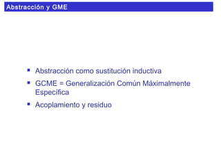
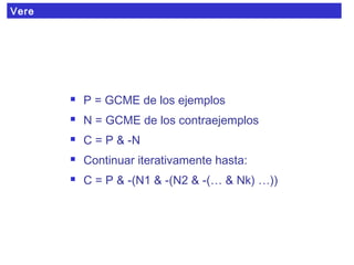
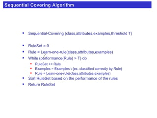
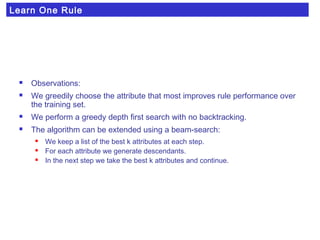
The document summarizes algorithms for learning first-order logic rules from examples, including: 1) A sequential covering algorithm that learns one rule at a time to cover examples, removing covered examples and repeating until all examples are covered or rules have low performance. 2) The learn-one-rule sub-algorithm uses a decision tree-like approach to greedily select the attribute that best splits examples according to a performance metric. 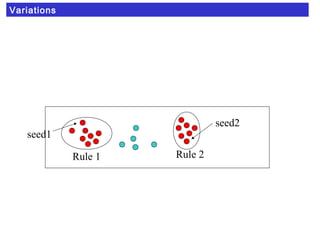3) Variations include allowing low probability classes and using a seed example approach instead of removing covered examples between rules.

1. Buenos Aires, mayo de 2016
Eduardo Poggi

2. Agenda
 Reglas de generalización
 Algoritmo Star de Michalsky
 Algoritmo de Vere
 Learning First Order Rules

3. Agenda
 Reglas de generalización
 Algoritmo Star de Michalsky
 Algoritmo de Vere
 Learning First Order Rules

4. Reglas de generalización
 Eliminación de conjunción
 P(X) <- A(X) ^ B(X) ^ C(X) <
 P(X) <- A(X) ^ B(X)
 Adición de disyunción
 P(X) <- A(X) <
 P(x) <- A(X) v B(X)
 Conjunciones por disyunciones
 P(X) <- A(X) ^ B(X) <
 P(x) <- A(X) v B(X)

5. Reglas de generalización
 Ampliación de rango de valores
 P(v/v in R1) <
 P(v/v in R2) iif R1<R2
 Constantes por variables
 P(a) <- <
 P(X) <-
 Resolución inductiva
 { P(X) <- A(X) ^ B(X);
 P(X) <- -A(X) ^ C(X) } <
 P(X) <- B(X) v C(X)

6. Reglas de generalización
 Escalar en árbol de
generalización
 P(v) <
 P(t(v)) iif v<t(v)

7. Distancias
ProductoProducto
ComestiblesComestibles LimpiezaLimpieza IndumentariaIndumentaria
AnimalAnimal VegetalVegetal MineralMineral
LácteosLácteos CárnicosCárnicos
Leche liquidaLeche liquida Leche fermentadaLeche fermentada QuesosQuesos MantecaManteca
Yogurt enteroYogurt entero Yogurt descremadoYogurt descremado
Yogurt naturalYogurt natural Yogurt saborizadoYogurt saborizado

8. Reglas de generalización constructivas
 Reemplazo de términos
 P(X) <- A(X) ^ B(X) <
 P(X) <- A(X) ^ C(X) iff B(X) < C(X)

9. Agenda
 Reglas de generalización
 Algoritmo Star de Michalsky
 Algoritmo de Vere
 Learning First Order Rules

10. STAR (Michalsky)
 Hasta condición de terminación
 Seleccionar un ejemplo
 Obtener el árbol de generalización (STAR) a partir de aplicar al
ejemplo todas las reglas de generalización (especialización)
posibles que no cubran contra-ejemplos.
 Evaluar la lista de generalización y ordenar.
 Eliminar los ejemplos ya cubiertos.

11. STAR (Michalsky)
venenoso(X) <-
color(X,marron)
forma(X,alargado)
tierra(X,humeda)
ambiente(X,humedo)
bajo_arbol(X,a33)
arbol(a33,fresno)
venenoso(X) <-
color(X,marron)
forma(X,alargado)
tierra(X,humeda)
ambiente(X,humedo)
bajo_arbol(X,a33)
arbol(a33,fresno)
venenoso(X) <-
color(X,marron)
forma(X,alargado)
tierra(X,humeda)
ambiente(X,humedo)
bajo_arbol(X,Y)
arbol(Y,fresno)
venenoso(X) <-
color(X,marron)
forma(X,alargado)
tierra(X,humeda)
ambiente(X,humedo)
bajo_arbol(X,Y)
arbol(Y,fresno)
venenoso(X) <-
color(X,marron)
forma(X,alargado)
tierra(X,humeda)
bajo_arbol(X,a33)
arbol(a33,fresno)
venenoso(X) <-
color(X,marron)
forma(X,alargado)
tierra(X,humeda)
bajo_arbol(X,a33)
arbol(a33,fresno)
venenoso(X) <-
color(X,marron)
forma(X,alargado)
tierra(X,humeda)
ambiente(X,humedo)
venenoso(X) <-
color(X,marron)
forma(X,alargado)
tierra(X,humeda)
ambiente(X,humedo)
venenoso(X) <- …venenoso(X) <- …

12. STAR (Michalsky)
venenoso(X) <- color(X,
[marron,verde])
forma(X,alargado)
tierra(X,humeda)
bajo_arbol(X,Y) arbol(Y,
[fresno,laurel])
venenoso(X) <- color(X,
[marron,verde])
forma(X,alargado)
tierra(X,humeda)
bajo_arbol(X,Y) arbol(Y,
[fresno,laurel])
venenoso(X) <-
forma(X,alargado)
tierra(X,humeda)
ambiente(X,humedo)
venenoso(X) <-
forma(X,alargado)
tierra(X,humeda)
ambiente(X,humedo)
venenoso(X) <-
color(X,marron)
forma(X,alargado)
tierra(X,humeda)
ambiente(X,humedo)
bajo_arbol(X,Y) arbol(Y,Z)
venenoso(X) <-
color(X,marron)
forma(X,alargado)
tierra(X,humeda)
ambiente(X,humedo)
bajo_arbol(X,Y) arbol(Y,Z)

13. Agenda
 Reglas de generalización
 Algoritmo Star de Michalsky
 Algoritmo de Vere
 Learning First Order Rules

14. Abstracción y GME
 Abstracción como sustitución inductiva
 GCME = Generalización Común Máximalmente
Específica
 Acoplamiento y residuo

15. Vere
 P = GCME de los ejemplos
 N = GCME de los contraejemplos
 C = P & -N
 Continuar iterativamente hasta:
 C = P & -(N1 & -(N2 & -(… & Nk) …))

16. Vere
 P1 =
 color(X,marron) ^ forma(X,alargado) ^ tierra(X,humeda) ^
 (ambiente(X,humedo) v ambiente(X,semi_humedo)^
 bajo_arbol(X,Y) ^ arbol(Y,Z)
 N1 =
 color(X,verde) ^ forma(X,redondo) ^
 ambiente(X,semi_humedo)^
 bajo_arbol(X,Y) ^ arbol(Y,Z)
 C1 = P1 ^ -N2 = ?

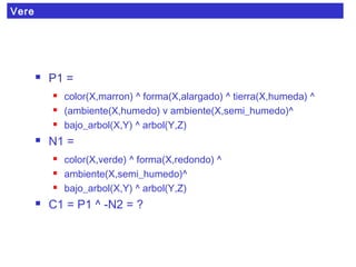
17. Vere
 C1 = P1 ^ -N2 =
 color(X,marron) ^ forma(X,alargado) ^ tierra(X,humeda) ^
 (ambiente(X,humedo) v ambiente(X,semi_humedo)^
 bajo_arbol(X,Y) ^ arbol(Y,Z) ^
 - [ color(X,verde) ^ forma(X,redondo) ^
 ambiente(X,semi_humedo) ^
 bajo_arbol(X,Y) ^ arbol(Y,Z) ]
 =
 color(X,marron) ^ forma(X,alargado) ^ tierra(X,humeda) ^
 (ambiente(X,humedo) v ambiente(X,semi_humedo) ^
 bajo_arbol(X,Y) ^ arbol(Y,Z) ^
 -color(X,verde) ^ -forma(X,redondo) ^
 -ambiente(X,semi_humedo) ^
 - bajo_arbol(X,Y) ^ - arbol(Y,Z)

18. Vere
 ≈ …
 color(X,marron) ^ -color(X,verde)
 forma(X,alargado) ^ -forma(X,redondo)
 tierra(X,humeda) ^
 ambiente(X,humedo ^
 bajo_arbol(X,Y) ^ arbol(Y,Z)

19. ML como BH
 K = ?
 Lista = {semilla}
 Hasta condición de terminación
 Nodo = primero de la lista
 Seleccionar reglas de generalización aplicables al Nodo
 Aplicar reglas al Nodo y generar nuevos Nodos
 Calcular Performance de Nodos
 Agregar Nodos a la Lista
 Ordenar Lista según Performance
 Truncar Lista en los k mejores

20. Agenda
 Reglas de generalización
 Algoritmo Star de Michalsky
 Algoritmo de Vere
 Learning First Order Rules

21. Learning set of rules
 Learning sets of rules has the advantage that the
hypothesis is easy to interpret.
 Sequential covering algorithm to learn first-order rules.

22. Learning rules
 First-order rule sets contain rules that have variables.
 This enables us to have stronger representational power.
 Example:
 If Parent(x,y) then Ancestor(x,y)
 If Parent(x,z) and Ancestor(z,y) then Ancestor(x,y)
 How would you represent this using a decision tree or predicate calculus?

23. Sequential Covering
 General idea:
 Learn one rule that covers certain number of positive examples
 Remove those examples covered by the rule
 Repeat until no positive examples are left.
Rule 1 Rule 2

24. Accuracy vs Coverage
We ask that each rule has high accuracy but not necessarily
high coverage, for example:
Rule 1
Rule 1 has 90% accuracy and 50% coverage. In general the
coverage may be low as long as accuracy is high.

25. Sequential Covering Algorithm
 Sequential-Covering (class,attributes,examples,threshold T)
 RuleSet = 0
 Rule = Learn-one-rule(class,attributes,examples)
 While (performance(Rule) > T) do
 RuleSet += Rule
 Examples = Examples {ex. classified correctly by Rule}
 Rule = Learn-one-rule(class,attributes,examples)
 Sort RuleSet based on the performance of the rules
 Return RuleSet

26. Sequential Covering Algorithm
 Observations:
 It performs a greedy search (no backtracking); as such it may not
find an optimal rule set.
 It learns a disjunctive set of rules by learning each disjunct
(conjunction of att.values) at a time.
 It sequentially covers the set of positive examples until the
performance of a rule is below a threshold.

27. Learn One Rule
How do we learn each individual rule?
One approach is to proceed as in decision tree learning but by
following the branch with best score in terms of splitting
function:
Luminosity
Mass
Type A Type B
Type C
> T1<= T1
> T2<= T2
If Luminosity <= T1 and
Mass > T2 then class is Type B

28. Learn One Rule
 Observations:
 We greedily choose the attribute that most improves rule performance over
the training set.
 We perform a greedy depth first search with no backtracking.
 The algorithm can be extended using a beam-search:
 We keep a list of the best k attributes at each step.
 For each attribute we generate descendants.
 In the next step we take the best k attributes and continue.

29. Algorithm
 LearnOneRule(class,attributes,examples,k):
 Best-hypothesis = 0
 Candidate-hypotheses = {Best-hypothesis}
 While Candidate-hypotheses is not empty do
 Generate the next more specific candidate hypotheses
 Update Best-hypothesis

For all h in new-candidates

if (Performance(h) > Performance(Best-hypothesis)) Best-hypothesis = h
 Update Candidate-hypotheses = best k members of new-candidates
 Return rule: If Best-hypothesis then prediction (most frequent class of
examples covered by Best-hypothesis)

30. Algorithm
 Generate the next more specific candidate hypotheses:
 Values = the set of all attribute values, e.g., color = blue
 For each rule h in Candidate-hypotheses do
 For each attribute-value v do

Add to h value v

new-candidates += h
 Remove from new-candidates hypotheses that are duplicates, inconsistent or
not maximally specific.
 Return new-candidates

31. Example
 Astronomy problem: classifying objects as stars of different types.
 Attributes: luminosity, mass, temperature, size.
 Assume the set of possible values are as follows:
 Luminosity <= T1 = l1 Luminosity > T1 = l2
 Mass <= T2 = m1 Mass > T2 = m2
 Temperature <= T3 = c1 Temperature > T3 = c2
 Size <= T4 = s1 Size > T4 = s2

32. Running Algorithm on Example
 Most specific hypotheses:
 l1, l2, m1, m2, c1, c2, s1, s2
 Assume Performance = P
 P(c1) > P(x) for all x different than c1
 Then best-hypothesis = c1
 Assume k = 4
 Best possible hypotheses: l1, m2, s1, c1

33. Running Algorithm on Example
 Candidate hypotheses: l1, m2, and c1
 New candidates:
 l1 & l1 (*)
 l1 & L2 (^) m2 & l1 c1 & l1
 l1 & m1 m2 & l2 c1 & l2
 l1 & m2 m2 & m1 (^) … etc
 l1 & c1 m2 & m2 (*)
 l1 & c2 m2 & c1
 l1 & s1 … etc
 l1 & s2
 (*) duplicate (^) inconsistent

34. Running Algorithm on Example
 Compute the performance of each new candidate.
 Update best-hypothesis to the best new candidate
 Example:
 Best–hypothesis = l1 & c2
 Now take the best k = 3 new candidates
 And continue generating new candidates:
 l1 & c2 & s1
 l1 & c2 & s2
 … etc

35. Performance Evaluation
 The performance of a new candidate can be computed
using information-theoretic measures like entropy:
 Performance(h, examples, class)
 h_examples = the subsets of examples covered by h
 Return Entropy(h_examples)

36. Considerations
 The best-hypothesis is the hypothesis with highest
 performance value, and not necessarily the last hypothesis:
 Space:
 L1, m2, c1
 L1&m2, l2&s1, m2&c1
 L1&m2&s1, l2&s1&c2, m2&c1&s2
 …
 Possible best hypothesis: l2&s1

37. Variations
What happens if the proportion of examples of a class is low?
In other words what happens if the a priori probability of a class
of examples is very low?
Example: patients with a very strange disease.
In that case we can modify the algorithm to learn only from those
rare examples, and to classify anything outside the rule set as negative.

38. Variations
 A second variation is used in the popular AQ and CN2 algorithms.
General idea:
 Choose one seed positive example
 Look for the most specific rule that covers the positive example and has
high performance
 Repeat with another seed example until no more improvement is seen on
the rule set

39. Variations
Rule 1 Rule 2
seed1
seed2

40. Final Points for Consideration
 A search can be done in a general-to-specific fashion. But one can also use
a specific-to-general fashion. Which one is best?
 Here we use a generate-then-test strategy. How about using an example-
driven strategy like the candidate elimination algorithm? (this last type is
more easily fooled by noise in the data)
 When and how should we prune rules?
 Different performance metrics exist:
 Relative frequency
 Accuracy
 Entropy

41. Rule learning and decision trees
 What is the difference between both?
 Decision trees: Divide and conquer
 Rule Learning: Separate and conquer

42. eduardopoggi@yahoo.com.ar
eduardo-poggi
http://ar.linkedin.com/in/eduardoapoggi
https://www.facebook.com/eduardo.poggi
@eduardoapoggi

43. Bibliografía