Scheduling Algorithms
Scheduling Algorithms FCFS
• First-come First-served (FCFS) (FIFO)
– Jobs are scheduled in order of arrival
– Non-preemptive
• Problem:
– Average waiting time depends on arrival order
• Advantage: really simple!
time
P1 P2 P3
0 16 20 24
P1P2 P3
0 4 8 24
Convoy Effect
• A CPU bound job will hold CPU until done,
– or it causes an I/O burst
• rare occurrence, since the thread is CPU-bound
⇒ long periods where no I/O requests issued, and CPU held
– Result: poor I/O device utilization
• Example: one CPU bound job, many I/O bound
• CPU bound runs (I/O devices idle)
• CPU bound blocks
• I/O bound job(s) run, quickly block on I/O
• CPU bound runs again
• I/O completes
• CPU bound still runs while I/O devices idle (continues…)
– Simple hack: run process whose I/O completed?
• What is a potential problem?
Scheduling Algorithms LIFO
• Last-In First-out (LIFO)
– Newly arrived jobs are placed at head of ready queue
– Improves response time for newly created threads
• Problem:
– May lead to starvation – early processes may never get
CPU
Problem
• You work as a short-order cook
– Customers come in and specify which dish they want
– Each dish takes a different amount of time to prepare
• Your goal:
– minimize average time the customers wait for their food
• What strategy would you use ?
– Note: most restaurants use FCFS.
Scheduling Algorithms: SJF
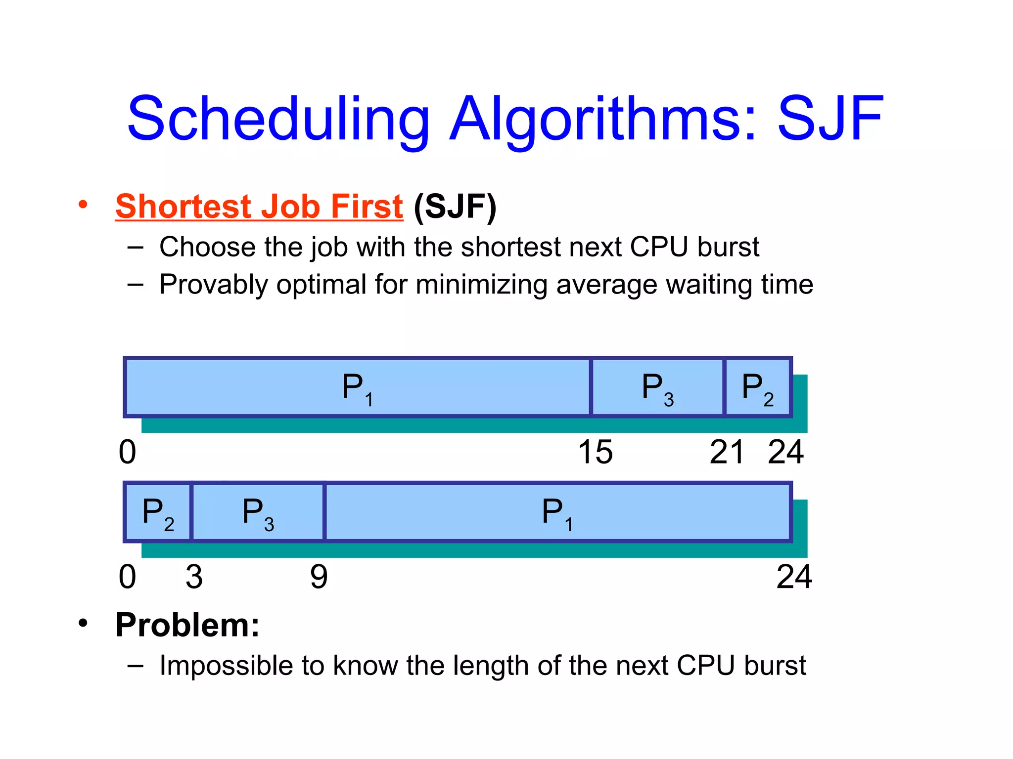
• Shortest Job First (SJF)
– Choose the job with the shortest next CPU burst
– Provably optimal for minimizing average waiting time
• Problem:
– Impossible to know the length of the next CPU burst
P1 P2P3
0 15 21 24
P1P2 P3
0 3 9 24
P2 P3
Scheduling Algorithms SRTF
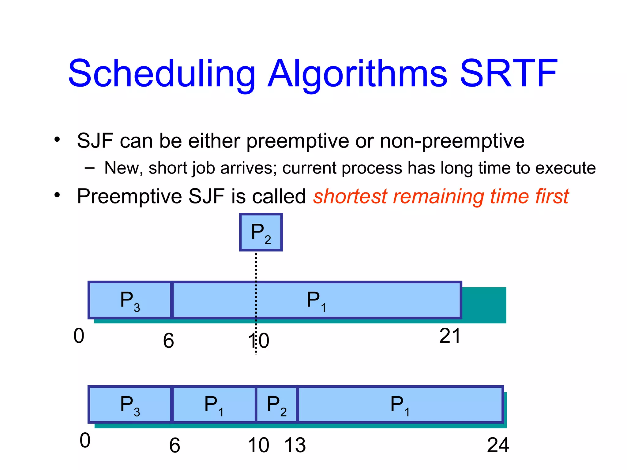
• SJF can be either preemptive or non-preemptive
– New, short job arrives; current process has long time to execute
• Preemptive SJF is called shortest remaining time first
P1
P2
P3
0 6 2110
P1P3 P1
P2
0 6 2410 13
• Approximate next CPU-burst duration
– from the durations of the previous bursts
• The past can be a good predictor of the future
• No need to remember entire past history
• Use exponential average:
tnduration of the nth
CPU burst
τn+1 predicted duration of the (n+1)st
CPU burst
τn+1 = α tn + (1- α) τn
where 0 ≤ α ≤ 1
α determines the weight placed on past behavior
Shortest Job First Prediction
Priority Scheduling
• Priority Scheduling
– Choose next job based on priority
– For SJF, priority = expected CPU burst
– Can be either preemptive or non-preemptive
• Problem:
– Starvation: jobs can wait indefinitely
• Solution to starvation
– Age processes: increase priority as a function of waiting time
Round Robin
• Round Robin (RR)
– Often used for timesharing
– Ready queue is treated as a circular queue (FIFO)
– Each process is given a time slice called a quantum
– It is run for the quantum or until it blocks
– RR allocates the CPU uniformly (fairly) across participants.
– If average queue length is n, each participant gets 1/n
RR with Time Quantum = 20
Process Burst Time
P1 53
P2 17
P3 68
P4 24
• The Gantt chart is:
• Higher average turnaround than SJF,
• But better response time
P1 P2 P3 P4 P1 P3 P4 P1 P3 P3
0 20 37 57 77 97 117 121 134 154 162
Turnaround Time w/ Time Quanta
RR: Choice of Time Quantum
• Performance depends on length of the timeslice
– Context switching isn’t a free operation.
– If timeslice time is set too high
• attempting to amortize context switch cost, you get FCFS.
• i.e. processes will finish or block before their slice is up anyway
– If it’s set too low
• you’re spending all of your time context switching between threads.
– Timeslice frequently set to ~100 milliseconds
– Context switches typically cost < 1 millisecond
Moral:
Context switch is usually negligible (< 1% per timeslice)
unless you context switch too frequently and lose all
productivity
Scheduling Algorithms
• Multi-level Queue Scheduling
• Implement multiple ready queues based on job “type”
– interactive processes
– CPU-bound processes
– batch jobs
– system processes
– student programs
• Different queues may be scheduled using different algos
• Intra-queue CPU allocation is either strict or proportional
• Problem: Classifying jobs into queues is difficult
– A process may have CPU-bound phases as well as interactive ones
Multilevel Queue Scheduling
System Processes
Interactive Processes
Batch Processes
Student Processes
Lowest priority
Highest priority
Scheduling Algorithms
• Multi-level Feedback Queues
• Implement multiple ready queues
– Different queues may be scheduled using different algorithms
– Just like multilevel queue scheduling, but assignments are not static
• Jobs move from queue to queue based on feedback
– Feedback = The behavior of the job,
• e.g. does it require the full quantum for computation, or
• does it perform frequent I/O ?
• Very general algorithm
• Need to select parameters for:
– Number of queues
– Scheduling algorithm within each queue
– When to upgrade and downgrade a job
Multilevel Feedback Queues
Quantum = 2
Quantum = 4
Quantum = 8
FCFS
Lowest priority
Highest priority
A Multi-level System
low
high
high
priority
timeslice
I/O bound jobs
CPU bound jobs
Thread Scheduling
Since all threads share code & data segments
• Option 1: Ignore this fact
• Option 2: Gang scheduling
– run all threads belonging to a process together (multiprocessor only)
– if a thread needs to synchronize with another thread
• the other one is available and active
• Option 3: Two-level scheduling:
– Medium level scheduler
– schedule processes, and within each process, schedule threads
– reduce context switching overhead and improve cache hit ratio
• Option 4: Space-based affinity:
– assign threads to processors (multiprocessor only)
– improve cache hit ratio, but can bite under low-load condition
Real-time Scheduling
• Real-time processes have timing constraints
– Expressed as deadlines or rate requirements
• Common RT scheduling policies
– Rate monotonic
• Just one scalar priority related to the periodicity of the job
• Priority = 1/rate
• Static
– Earliest deadline first (EDF)
• Dynamic but more complex
• Priority = deadline
• Both require admission control to provide guarantees
Postscript
• The best schemes are adaptive.
• To do absolutely best we’d have to predict the future.
– Most current algorithms give highest priority to those that need
the least!
• Scheduling become increasingly ad hoc over the years.
– 1960s papers very math heavy, now mostly “tweak and see”
Problem
• What are metrics that schedulers should optimize for ?
– There are many, the right choice depends on the context
• Suppose:
– You own an airline, have one expensive plane, and passengers
waiting all around the globe
– You own a sweatshop, and need to evaluate workers
– You are at a restaurant, and are waiting for food
– You are an efficiency expert, and are evaluating government
procedures at the DMV
– You are trying to find a project partner or a co-author
– You own a software company that would like to deliver a product
by a deadline

Planificacion

  • 1.
  • 2.
    Scheduling Algorithms FCFS •First-come First-served (FCFS) (FIFO) – Jobs are scheduled in order of arrival – Non-preemptive • Problem: – Average waiting time depends on arrival order • Advantage: really simple! time P1 P2 P3 0 16 20 24 P1P2 P3 0 4 8 24
  • 3.
    Convoy Effect • ACPU bound job will hold CPU until done, – or it causes an I/O burst • rare occurrence, since the thread is CPU-bound ⇒ long periods where no I/O requests issued, and CPU held – Result: poor I/O device utilization • Example: one CPU bound job, many I/O bound • CPU bound runs (I/O devices idle) • CPU bound blocks • I/O bound job(s) run, quickly block on I/O • CPU bound runs again • I/O completes • CPU bound still runs while I/O devices idle (continues…) – Simple hack: run process whose I/O completed? • What is a potential problem?
  • 4.
    Scheduling Algorithms LIFO •Last-In First-out (LIFO) – Newly arrived jobs are placed at head of ready queue – Improves response time for newly created threads • Problem: – May lead to starvation – early processes may never get CPU
  • 5.
    Problem • You workas a short-order cook – Customers come in and specify which dish they want – Each dish takes a different amount of time to prepare • Your goal: – minimize average time the customers wait for their food • What strategy would you use ? – Note: most restaurants use FCFS.
  • 6.
    Scheduling Algorithms: SJF •Shortest Job First (SJF) – Choose the job with the shortest next CPU burst – Provably optimal for minimizing average waiting time • Problem: – Impossible to know the length of the next CPU burst P1 P2P3 0 15 21 24 P1P2 P3 0 3 9 24 P2 P3
  • 7.
    Scheduling Algorithms SRTF •SJF can be either preemptive or non-preemptive – New, short job arrives; current process has long time to execute • Preemptive SJF is called shortest remaining time first P1 P2 P3 0 6 2110 P1P3 P1 P2 0 6 2410 13
  • 8.
    • Approximate nextCPU-burst duration – from the durations of the previous bursts • The past can be a good predictor of the future • No need to remember entire past history • Use exponential average: tnduration of the nth CPU burst τn+1 predicted duration of the (n+1)st CPU burst τn+1 = α tn + (1- α) τn where 0 ≤ α ≤ 1 α determines the weight placed on past behavior Shortest Job First Prediction
  • 9.
    Priority Scheduling • PriorityScheduling – Choose next job based on priority – For SJF, priority = expected CPU burst – Can be either preemptive or non-preemptive • Problem: – Starvation: jobs can wait indefinitely • Solution to starvation – Age processes: increase priority as a function of waiting time
  • 10.
    Round Robin • RoundRobin (RR) – Often used for timesharing – Ready queue is treated as a circular queue (FIFO) – Each process is given a time slice called a quantum – It is run for the quantum or until it blocks – RR allocates the CPU uniformly (fairly) across participants. – If average queue length is n, each participant gets 1/n
  • 11.
    RR with TimeQuantum = 20 Process Burst Time P1 53 P2 17 P3 68 P4 24 • The Gantt chart is: • Higher average turnaround than SJF, • But better response time P1 P2 P3 P4 P1 P3 P4 P1 P3 P3 0 20 37 57 77 97 117 121 134 154 162
  • 12.
    Turnaround Time w/Time Quanta
  • 13.
    RR: Choice ofTime Quantum • Performance depends on length of the timeslice – Context switching isn’t a free operation. – If timeslice time is set too high • attempting to amortize context switch cost, you get FCFS. • i.e. processes will finish or block before their slice is up anyway – If it’s set too low • you’re spending all of your time context switching between threads. – Timeslice frequently set to ~100 milliseconds – Context switches typically cost < 1 millisecond Moral: Context switch is usually negligible (< 1% per timeslice) unless you context switch too frequently and lose all productivity
  • 14.
    Scheduling Algorithms • Multi-levelQueue Scheduling • Implement multiple ready queues based on job “type” – interactive processes – CPU-bound processes – batch jobs – system processes – student programs • Different queues may be scheduled using different algos • Intra-queue CPU allocation is either strict or proportional • Problem: Classifying jobs into queues is difficult – A process may have CPU-bound phases as well as interactive ones
  • 15.
    Multilevel Queue Scheduling SystemProcesses Interactive Processes Batch Processes Student Processes Lowest priority Highest priority
  • 16.
    Scheduling Algorithms • Multi-levelFeedback Queues • Implement multiple ready queues – Different queues may be scheduled using different algorithms – Just like multilevel queue scheduling, but assignments are not static • Jobs move from queue to queue based on feedback – Feedback = The behavior of the job, • e.g. does it require the full quantum for computation, or • does it perform frequent I/O ? • Very general algorithm • Need to select parameters for: – Number of queues – Scheduling algorithm within each queue – When to upgrade and downgrade a job
  • 17.
    Multilevel Feedback Queues Quantum= 2 Quantum = 4 Quantum = 8 FCFS Lowest priority Highest priority
  • 18.
  • 19.
    Thread Scheduling Since allthreads share code & data segments • Option 1: Ignore this fact • Option 2: Gang scheduling – run all threads belonging to a process together (multiprocessor only) – if a thread needs to synchronize with another thread • the other one is available and active • Option 3: Two-level scheduling: – Medium level scheduler – schedule processes, and within each process, schedule threads – reduce context switching overhead and improve cache hit ratio • Option 4: Space-based affinity: – assign threads to processors (multiprocessor only) – improve cache hit ratio, but can bite under low-load condition
  • 20.
    Real-time Scheduling • Real-timeprocesses have timing constraints – Expressed as deadlines or rate requirements • Common RT scheduling policies – Rate monotonic • Just one scalar priority related to the periodicity of the job • Priority = 1/rate • Static – Earliest deadline first (EDF) • Dynamic but more complex • Priority = deadline • Both require admission control to provide guarantees
  • 21.
    Postscript • The bestschemes are adaptive. • To do absolutely best we’d have to predict the future. – Most current algorithms give highest priority to those that need the least! • Scheduling become increasingly ad hoc over the years. – 1960s papers very math heavy, now mostly “tweak and see”
  • 22.
    Problem • What aremetrics that schedulers should optimize for ? – There are many, the right choice depends on the context • Suppose: – You own an airline, have one expensive plane, and passengers waiting all around the globe – You own a sweatshop, and need to evaluate workers – You are at a restaurant, and are waiting for food – You are an efficiency expert, and are evaluating government procedures at the DMV – You are trying to find a project partner or a co-author – You own a software company that would like to deliver a product by a deadline