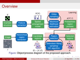
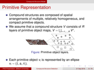
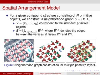
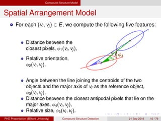
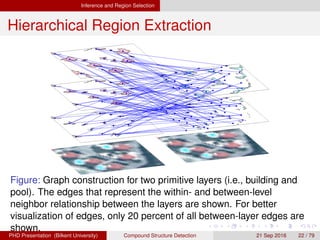
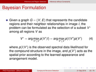
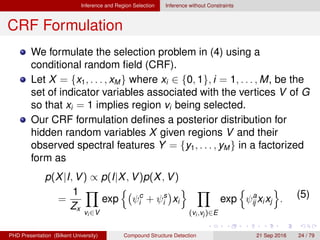
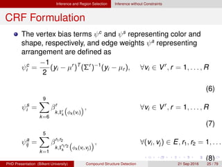
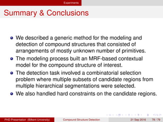
This document proposes a method for automatically detecting compound structures from multiple hierarchical segmentations of remote sensing images. Compound structures contain spatial arrangements of primitive objects like buildings, trees, and roads. The method models compound structures as probabilistic region processes and learns their appearance and spatial models from training data. Candidate regions are extracted from hierarchical segmentations, and a constrained region selection framework is used to detect compound structure instances by selecting coherent subsets of regions that satisfy constraints. Approximate inference is performed using Markov chain Monte Carlo sampling or quadratic programming under constraints.


![Learning
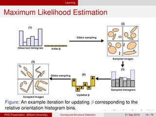
Maximum Likelihood Estimation
Suppose that we observe a set of i.i.d. region processes
V = {V1, . . . , VM}.
We can estimate a compound structure model via
maximum likelihood estimation (MLE) of β by maximizing
(β|V) =
M
m=1
log p(Vm|β). (2)
The gradient of the log-likelihood is given by
d (β|V)
dβ
= Ep[H(V)] −
1
M
N
m=1
H(Vm). (3)
We use the stochastic gradient ascent algorithm where the
expectation Ep[H(V)] is approximated by a finite sum of
histograms of samples V(s), s = 1, . . . , S.
H. G. Akc¸ay Compound Structure Detection 21 Sept. 2016 15 / 78](https://image.slidesharecdn.com/thesispresentation-170131124202/85/Compound-Structure-Detection-15-320.jpg)


![[IJET-V1I3P9] Authors :Velu.S, Baskar.K, Kumaresan.A, Suruthi.K](https://cdn.slidesharecdn.com/ss_thumbnails/ijet-v1i3p9-150603165341-lva1-app6892-thumbnail.jpg?width=640&height=640&fit=bounds)


