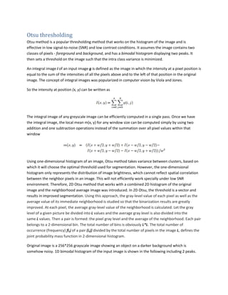
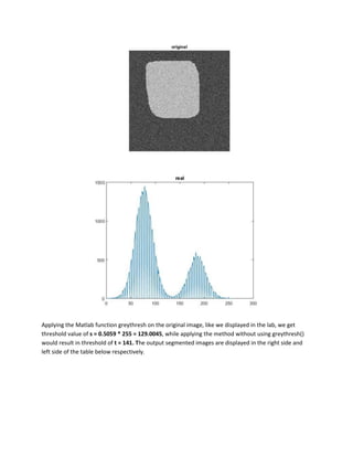
Otsu thresholding is an effective thresholding method for images with low signal-to-noise ratios and low contrast. It assumes a bimodal histogram with two peaks, foreground and background, and finds a threshold that minimizes intra-class variance. 2D Otsu thresholding uses a joint 2D histogram of pixel values and local neighborhood averages to find an optimal threshold vector, improving segmentation especially for noisy images. The algorithm calculates the 2D histogram, finds probabilities and mean values, and selects the threshold pair that maximizes between-class variance. On a noisy test image, 2D Otsu thresholding produces a clean binary segmentation with the threshold pair (171, 171).

1. Otsu thresholding
Otsu method is a popular thresholding method that works on the histogram of the image and is
effective in low signal-to-noise (SNR) and low contrast conditions. It assumes the image contains two
classes of pixels - foreground and background, and has a bimodal histogram displaying two peaks. It
then sets a threshold on the image such that the intra class variance is minimized.
An integral image i of an input image g is defined as the image in which the intensity at a pixel position is
equal to the sum of the intensities of all the pixels above and to the left of that position in the original
image. The concept of integral images was popularized in computer vision by Viola and Jones.
So the intensity at position (x, y) can be written as
The integral image of any greyscale image can be efficiently computed in a single pass. Once we have
the integral image, the local mean m(x, y) for any window size can be computed simply by using two
addition and one subtraction operations instead of the summation over all pixel values within that
window
Using one-dimensional histogram of an image, Otsu method takes variance between clusters, based on
which it will choose the optimal threshold used for segmentation. However, the one-dimensional
histogram only represents the distribution of image brightness, which cannot reflect spatial correlation
between the neighbor pixels in an image. This will not efficiently work specially under low SNR
environment. Therefore, 2D Otsu method that works with a combined 2D histogram of the original
image and the neighborhood average image was introduced. In 2D Otsu, the threshold is a vector and
results in improved segmentation. Using this approach, the gray-level value of each pixel as well as the
average value of its immediate neighborhood is studied so that the binarization results are greatly
improved. At each pixel, the average gray-level value of the neighborhood is calculated. Let the gray
level of a given picture be divided into L values and the average gray level is also divided into the
same L values. Then a pair is formed: the pixel gray level and the average of the neighborhood. Each pair
belongs to a 2-dimensional bin. The total number of bins is obviously L*L. The total number of
occurrence (frequency) fi,j of a pair (i,j) divided by the total number of pixels in the image L, defines the
joint probability mass function in 2-dimensional histogram.
Original image is a 256*256 grayscale image showing an object on a darker background which is
somehow noisy. 1D bimodal histogram of the input image is shown in the following including 2 peaks.

2. Applying the Matlab function greythresh on the original image, like we displayed in the lab, we get
threshold value of s = 0.5059 * 255 = 129.0045, while applying the method without using greythresh()
would result in threshold of t = 141. The output segmented images are displayed in the right side and
left side of the table below respectively.

3. clear;
clc;
format compact;
im_org=double(imread('16.bmp'));
size(im_org)
im_pro=im_org-min(im_org(:));
im_pro=round(im_pro*(255/max(im_pro(:))));
figure(10);imagesc(im_pro);colormap(gray);axis image;axis off;
title('original');
I=im_pro/255;
s=graythresh(I)
x=im2bw(I,s);
figure(11);imagesc(x);colormap(gray);axis image;title('Otsu');
xlabel(num2str(255*s));
h=zeros(0,255);
for i=0:255
temp=find(im_pro==i);
h(i+1)=numel(temp);
end
figure(12);plot(1+log(h));title('logvar');
he=zeros(0,255);
for i=0:255
temp=find(im_pro==i);
he(i+1)=numel(temp);
end
figure(13);plot(he);title('real');
sumOfVar=zeros(1,254);
for i=1:254
Ib=im_pro(im_pro<=i);
Io=im_pro(im_pro>i);
sumOfVar(i)=var(Ib)+var(Io);
end
figure(14);plot(sumOfVar);title('var');

4. t=find(sumOfVar==min(sumOfVar));
t=mean(t)
im_pro(im_pro<t)=0;
im_pro=sign(im_pro);
figure(15);imagesc(im_pro);colormap(gray);axis image;xlabel('us');
2D-histogram based Otsu:
According to introduction in first page, 2D histogram of gray scale image is required in order for
calculating the threshold vector. First, drawing 2D histogram using blurred image of the input image:
 hist2d is 256*256 2D-histogram of grayscale value and neighborhood average value pair
 total is the number of pairs in the given image
 threshold is the threshold obtained

5. The 2D histogram is calculated and displayed using mesh plotting:
fontSize = 10;
grayImage = imread('16.bmp');
figure(2);
imshow(grayImage, []);
title('Original Grayscale Image', 'FontSize', fontSize);
% Let's compute and display the histogram.
[pixelCount, grayLevels] = imhist(grayImage);
figure(3);
bar(grayLevels, pixelCount);

6. grid on;
title('Histogram of original image', 'FontSize', fontSize);
xlim([0 grayLevels(end)]); % Scale x axis manually.
% Get the local average image
windowWidth = 21;
kernel = ones(windowWidth)/windowWidth^2;
blurredImage = imfilter(grayImage, kernel);
% Display the original gray scale image.
figure(4);
imshow(blurredImage, []);
title('Blurred Grayscale Image', 'FontSize', fontSize);
% Compute the 2D "histogram"
[rows, columns, numberOfColorBands] = size(grayImage);
hist2d = zeros(256,256);
for row = 1 : rows
for column = 1 : columns
index1 = grayImage(row, column);
index2 = round(blurredImage(row, column));
hist2d(index1, index2) = hist2d(index1, index2) + 1;
end
end
figure(5);
%imshow(hist2d, []);
mesh(hist2d);
title('2D Histogram', 'FontSize', fontSize);
[x,y] = meshgrid([0, 255]);
size(hist2d)
%Finding Otsu threshold:
% hist2d is the 256*256 2D-histogram of grayscale value and neighborhood
average grayscale value pair.
% total is the number of pairs in the given image.
% threshold is the threshold obtained.
hist2dmax=max(hist2d(:))
maximum = 0.0;
threshold = 0;
helperVec = 0:255;
mu_t0 = sum(sum(repmat(helperVec',1,256).*hist2d));
mu_t1 = sum(sum(repmat(helperVec,256,1).*hist2d));
p_0 = zeros(256);
mu_i = p_0;
mu_j = p_0;
total = hist2dmax;
for ii = 2:256
for jj = 2:256
if jj == 2
if ii == 2
p_0(2,2) = hist2d(2,2);
else
p_0(ii,1) = p_0(ii-1,1) + hist2d(ii,1);
mu_i(ii,1) = mu_i(ii-1,1)+(ii-1)*hist2d(ii,1);
mu_j(ii,1) = mu_j(ii-1,1);
end
else
p_0(ii,jj) = p_0(ii,jj-1)+p_0(ii-1,jj)-p_0(ii-1,jj-

7. 1)+hist2d(ii,jj);
mu_i(ii,jj) = mu_i(ii,jj-1)+mu_i(ii-1,jj)-mu_i(ii-1,jj-1)+(ii-
1)*hist2d(ii,jj);
mu_j(ii,jj) = mu_j(ii,jj-1)+mu_j(ii-1,jj)-mu_j(ii-1,jj-1)+(jj-
1)*hist2d(ii,jj);
end
if (p_0(ii,jj) == 0)
continue;
end
if (p_0(ii,jj) == hist2dmax)
break;
end
tr = ((mu_i(ii,jj)-p_0(ii,jj)*mu_t0)^2 + (mu_j(ii,jj)-
p_0(ii,jj)*mu_t0)^2)/(p_0(ii,jj)*(1-p_0(ii,jj)));
if ( tr >= maximum )
threshold = ii;
maximum = tr;
end
end
end
threshold = threshold / 255
2D Otsu algorithm:
2D histogram is depicted according to the frequency of pairs appeared in the original image:

8. hmax = 2.6751e+03
The threshold pair is calculated as s = 171, t = 171. In addition, Elapsed time is 0.437781 seconds using
tic toc. The output segmented image is displayed below, showing a clean representation of the noisy
original image with clear segmentation of foreground (object) and background.
tic
a=imread('16.bmp'); %Read a image
%a=a(:,:,1);

9. % % a=M;
% %load('source_N0.02.mat');
% %a=X;
%a=imread('syn1-g2.gif');
%a=b;
%a=noise_h;
figure(6);
imshow(a);
[m,n]=size(a);
%b=imnoise(a,'salt & pepper',0.003);
%b=imnoise(b,'gaussian',0,0.0015);
%b = IMNOISE(a,'speckle',0.09);
%b=a;
a0=double(a);
h=1;
a1=zeros(m,n);
for i=1:m ...rows
for j=1:n ...columns
for k=-h:h ...3by3 window
for w=-h:h;
p=i+k;
q=j+w;
if (p<=0)|( p>m) ...not to exceed image rows
p=i;
end
if (q<=0)|(q>n) ...not to exceed image columns
q=j;
end
a1(i,j)=a0(p,q)+a1(i,j);
end
end
a2(i,j)=uint8(1/9*a1(i,j)); ...neighbourhood average image
represented by grey levels
end
end
% 2D histogram representation:
% f denotes the frequency of a pair appeared in the image
fxy=zeros(256,256);
for i=1:m
for j=1:n
c=a0(i,j);
d=double(a2(i,j));
fxy(c+1,d+1)=fxy(c+1,d+1)+1;
end
end
figure(7);
mesh(fxy);
title('2D Hist');
% to obtain a pair, P, composed by original intensity and the average
intensity
Pxy=fxy/m/n;
P0=zeros(256,256);
Ui=zeros(256,256);
Uj=zeros(256,256);
P0(1,1)=Pxy(1,1);

10. for i=2:256
P0(1,i)=P0(1,i-1)+Pxy(1,i);
end
for i=2:256
P0(i,1)=P0(i-1,1)+Pxy(i,1);
end
for i=2:256
for j=2:256
P0(i,j)=P0(i,j-1)+P0(i-1,j)-P0(i-1,j-1)+Pxy(i,j);
end
end
P1=ones(256,256)-P0;
Ui(1,1)=0;
for i=2:256
Ui(1,i)=Ui(1,i-1)+(1-1)*Pxy(1,i);
end
for i=2:256
Ui(i,1)=Ui(i-1,1)+(i-1)*Pxy(i,1);
end
for i=2:256
for j=2:256
Ui(i,j)=Ui(i,j-1)+Ui(i-1,j)-Ui(i-1,j-1)+(i-1)*Pxy(i,j);
end
end
Uj(1,1)=0;
for i=2:256
Uj(1,i)=Uj(1,i-1)+(i-1)*Pxy(1,i);
end
for i=2:256
Uj(i,1)=Uj(i-1,1)+(1-1)*Pxy(i,1);
end
for i=2:256
for j=2:256
Uj(i,j)=Uj(i,j-1)+Uj(i-1,j)-Uj(i-1,j-1)+(j-1)*Pxy(i,j);
end
end
uti=0;
utj=0;
for i=1:256
for j=1:256
uti=uti+(i-1)*Pxy(i,j);
utj=utj+(j-1)*Pxy(i,j);
end
end
% for i=1:256
% for j=1:256
% Ui1(i,j)=Ui(256,256)-Ui(i,j);
% Uj1(i,j)=Uj(256,256)-Uj(i,j);
% end
% end
hmax=0;
for i=1:256
for j=1:256
if P0(i,j)~=0&P1(i,j)~=0
h(i,j)=((uti*P0(i,j)-Ui(i,j))^2+(utj*P0(i,j)-
Uj(i,j))^2)/(P1(i,j)*P0(i,j));
else

11. h(i,j)=0;
end
end
end
hmax=max(h(:));
for i=1:256
for j=1:256
if h(i,j)==hmax
s=i-1;
t=j-1;
continue;
end
end
end
hmax
s
t
% Applying threshold on the input image
z=ones(m,n);
%c=zeros(m,n);
for i=1:m
for j=1:n
if a(i,j)<=s&a2(i,j)<=t
%if double(b(i,j))+double(a2(i,j))<=s+t
z(i,j)=0;
end
end
end
figure(8);
imshow(z);
toc