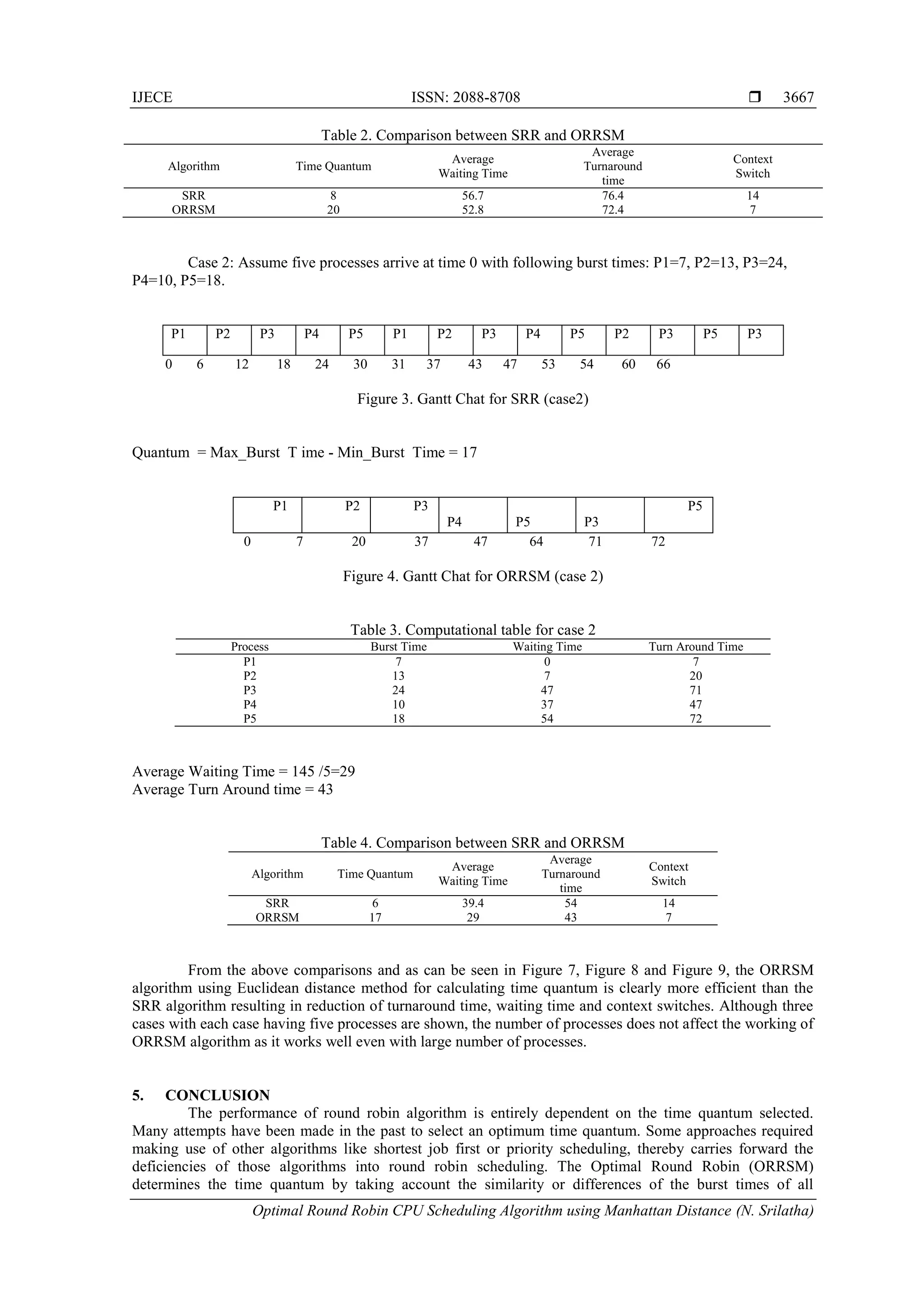
This document presents an optimal round robin CPU scheduling algorithm that uses Manhattan distance to determine the time quantum, aiming to balance the CPU utilization and response time. The proposed algorithm offers improved performance over the classic round robin algorithm by reducing context switches, average waiting time, and turnaround time. The findings from experimental analyses indicate the clear efficiency of the new method compared to traditional approaches.
![International Journal of Electrical and Computer Engineering (IJECE)
Vol. 7, No. 6, December 2017, pp. 3664~3668
ISSN: 2088-8708, DOI: 10.11591/ijece.v7i6.pp3664-3668 3664
Journal homepage: http://iaesjournal.com/online/index.php/IJECE
Optimal Round Robin CPU Scheduling Algorithm using
Manhattan Distance
N. Srilatha1
, M. Sravani 2
, Y. Divya3
Department of Computer Science and Engineering, RGUKT, AP IIIT, Idupulapya, Kadapa, Andhrapradhesh
Article Info ABSTRACT
Article history:
Received Mar 23, 2017
Revised Sep 8, 2017
Accepted Sep 25, 2017
In Round Robin Scheduling the time quantum is fixed and then processes are
scheduled such that no process get CPU time more than one time quantum in
one go. The performance of Round robin CPU scheduling algorithm is
entirely dependent on the time quantum selected. If time quantum is too
large, the response time of the processes is too much which may not be
tolerated in interactive environment. If time quantum is too small, it causes
unnecessarily frequent context switch leading to more overheads resulting in
less throughput. In this paper a method using Manhattan distance has been
proposed that decides a quantum value. The computation of the time
quantum value is done by the distance or difference between the highest
burst time and lowest burst time. The experimental analysis also shows that
this algorithm performs better than RR algorithm and by reducing number of
context switches, reducing average waiting time and also the average turna
round time.
Keyword:
Round robin
Quantum
Scheduling
Burst times
Copyright © 2017Institute of Advanced Engineering and Science.
All rights reserved.
Corresponding Author:
N. Srilatha,
Department of Computer Science and Engineering,
RGUKT-AP IIIT,
RK Valley, Idupulapaya, Kadapa, Andhrapradhesh.
Email: srilathargukt16@gmail.com
1. INTRODUCTION
The Central Processing Unit (CPU) should be utilized efficiently as it is the core part of Computers.
For this reason CPU scheduling is very necessary. CPU Scheduling is a important concept in Operating
System. Sharing of computer resources between multiple processes is called scheduling. The Scheduling
operation is done by the scheduler. In operating system we have three types of schedulers [1]. The types of
the schedulers depend on the context switches of the process. They are 1. Longterm Scheduler 2. Short term
Scheduler 3. Medium term scheduler. Here are several scheduling algorithms. Different scheduling
algorithms have different properties and the choice of a particular algorithm may favor one class of processes
over another. Many criteria have been suggested for comparing CPU scheduling algorithms and deciding
which one is the best algorithm [1]. Some of the criteria include (i) Fairness (i) CPU utilization (iii)
Throughput (iv)T urnaround time (v) Waiting time (vi) Response time. It is desirable to maximize CPU
utilization and throughput, to minimize turnaround time, waiting time and response time and to avoid
starvation of any process. [1, 2] Some of the scheduling algorithms are briefly described below: FCFS: In
First come First serve scheduling algorithm the process that request first is scheduled for execution [1, 2, 3]
SJF: In shortest Job first scheduling algorithm the process with the minimum burst time is scheduled for
execution. [1, 2] SRTN: In shortest Remaining time next scheduling algorithm, the process with shortest
remaining time is scheduled for execution. [3] Priority: in Priority Scheduling algorithm the process with
highest priority is scheduled for execution. [1, 2, 3] Multilevel queue scheduling: In this the ready queue is
partitioned into several separate queues. The processes are permanently assigned to one queue generally
based on some property of the process such as memory size, process priority or process type. Each queue has](https://image.slidesharecdn.com/v838sep1723mar15241-30220rredit-201104030239/75/Optimal-Round-Robin-CPU-Scheduling-Algorithm-using-Manhattan-Distance-1-2048.jpg)
![IJECE ISSN: 2088-8708
Optimal Round Robin CPU Scheduling Algorithm using Manhattan Distance (N. Srilatha)
3665
its own scheduling algorithm. There is scheduling among the queues, which is commonly implemented as
fixed-priority preemptive scheduling. Each queue has absolute priority over low priority queues. [1]
Multilevel feedback-queue scheduling: This is like Multilevel queue scheduling but allows a process to
move between queues. [3] Round-robin: In this the CPU scheduler goes around the ready queue allocating
the CPU to each process for a time interval of up to one time quantum. If time quantum is too large, the
response time of the processes is too much which may not be tolerated in interactive environment. If time
quantum is too small, it causes unnecessarily frequent context switch leading to more overheads resulting in
less throughput. In this paper a method using Manhattan distance logic has been proposed that decides a
value that is neither too large nor too small such that every process has got reasonable response time and the
throughput of the system is not decreased due to unnecessarily context switches.
The various scheduling parameters are:
1. Context Switch: A context switch is basically storing and restoring context or state of a pre-empted
process, so that at a later point of time , it can be started from same point once the execution is stopped.
So the goal of CPU scheduling algorithms is to optimize only these switches.
2. Throughput: Throughput is defined as number of processes completed in a period of time. Context
switching and Throughput are inversely proportional to each other.
3. CPU Utilization: This is the fraction of time when CPU is in use. Usually, to maximize the CPU
utilization is the goal of the CPU scheduling
4. Turnaround Time: This is the total time which is required to spend to complete the whole process and
amount of time it takes to execute that process.
5. Waiting Time: Waiting time is defined as the total amount of time a process that waits in ready queue.
6. Response Time: For responding to a particular system the amount of time used by the system.
The characteristic of good scheduling algorithm are:
Minimum context switches, Maximum CPU utilization, Maximum throughput, Minimum turnaround time,
Minimum waiting time
2. BACKGROUND WORK
There is a host of work and researches going on for increasing the efficiency of round robin
algorithm. Rami J. Matarneh [4] proposed a method that calculates median of burst time of all processes in
ready queue. Now if this median is less than 25 than time quantum would be 25 otherwise time quantum is
set to the calculated value. Ahad [5] proposed to modify the time quantum of a process based on some
threshold value which is calculated by taking average of left out time of all processes in its last turn.
Hiranwal et al. [6] introduced a concept of smart time slice which is calculated by taking the average of burst
time of all processes in the ready queue if number of processes are even otherwise time slice is set to mid
process burst time. Dawood [7] proposed an algorithm that first sorts all processes in ready queue and then
calculate the time quantum by multiplying sum of maximum and minimum burst by 80. Noon et al [8]
proposed to calculate the time quantum by taking average of the burst time of all the processes in ready
queue. Banerjee et al [9] proposed an algorithm which first sorts all the processes according to the burst time
and then finds the time quantum by taking average of burst time of all process from mid to last. Nayak et al.
[10] calculated the optimal time quantum by taking the average of highest burst and median of burst.
Yaashuwanth et al [11] introduced a term intelligent time slice which is calculated using the formula (range
of burst * total number of processes)/ (priority range * Total number of priority). Matthias et al. [12]
proposed a solution for Linux SCHED_RR, to assign equal share of CPU to different users instead of
process. Racu et al. [13] presents an approach to compute best case and worst case response time of round
robin scheduling. In Merywns et al [14] used Euclidian distance for calculating Quantum value. In [15] in
this section, a non-linear mathematical model for optimizing the time quantum value in RR scheduling
algorithm is proposed.
In this paper we approached the Round Robin Quantum value using the Manhattan Distance.
Quantum value = Highest Burst time – Lowest Burst time.
3. PROPOSED WORK
A major disadvantage of round robin is that a process is pre-empted and context switch occurs, even
if the running process requires time (in fractions) which is slightly more than assigned time quantum.
Another problem with round robin is the time quantum selection. If time quantum is too large, the response
time of the processes is too much, the algorithm degenerates to FCFS which may not be tolerated in an
interactive environment. If time quantum is too small, it causes unnecessarily frequent context switches
leading to more overheads resulting in lesser throughput](https://image.slidesharecdn.com/v838sep1723mar15241-30220rredit-201104030239/75/Optimal-Round-Robin-CPU-Scheduling-Algorithm-using-Manhattan-Distance-2-2048.jpg)
![ ISSN:2088-8708
IJECE Vol. 7, No. 6, December 2017 : 3664–3668
3668
processes present in the ready queue. The ORRSM does not require priorities to be assigned to the jobs nor
does it require the jobs to be sorted according to their burst times. It results in better performance of round
robin algorithm with reduction in context switches, turnaround times and waiting times. The time quantum
determined through ORRSM is dynamic in the sense that no user intervention is required and the time
quantum is related to the burst times of processes.
REFERENCES
[1] Silberschatz, A., Peterson, J.L., and Galvin, P.B., Operating System Concepts, Addison Wesley, 7th Edition, 2006.
[2] Andrew S. Tanenbaum, and Albert S. Woodfhull, Operating Systems Design and Implementation, Second Edition,
2005.
[3] William Stallings, Operating Systems Internal and Design Principles, 5th Edition, 2006.
[4] Rami J Matarneh, “Self adjustment time quantum in round robin algorithm depending on burst time of the now
running process”, American Journal.
[5] Mohd Abdul Ahad, “Modifying round robin algorithm for process scheduling using dynamic quantum precision”,
International Journal of Computer applications(0975-8887) on Issues and Challenges in Networking, Intelligence
and Computing Technologies- ICNICT 2012.
[6] Saroj Hiranwal and Dr. K.C. Roy, “Adaptive round robin scheduling using shortest burst approach based on smart
time slice”, International Journal of Data Engineering, volume 2, Issue. 3, 2011.
[7] Ali Jbaeer Dawood, “Improving efficiency of round robin scheduling using ascending quantum and minimum-
maximum burst time”, Journal of University of anbar for pure science: Vol. 6: No 2, 2012.
[8] Abbas Noon, Ali Kalakech and Saifedine Kadry, “A new round robin based scheduling algorithm for operating
systems: dynamic quantum using the mean average”, IJCSI International Journal of Computer Science Issues, Vol.
8, Issue 3, No. 1, May 2011.
[9] Pallab Banerjee, Probal Banerjee and Shweta Sonali Dhal, “Comparative performance analysis of mid average
round robin scheduling (MARR) using dynamic time quantum with round robin scheduling algorithm having static
time quatum”, International Journal of Electronics and Computer Science Engineering, ISSN-2277-1956 2012.
[10] Debashree Nayak, Sanjeev Kumar Malla and Debashree Debadarshini, “Improved round robin scheduling using
dynamic time quantum”, International Journal of Computer Applications (0975-8887) Volume 38- No 5, January
2012.
[11] Yaashuwanth C. & R. Ramesh, “ Intelligent time slice for round robin in real time operating system, IJRRAS 2 (2),
February 2010.
[12] Braunhofer Matthias, Strum flohner Juri, “Fair round robin scheduling”, September 17, 2009.
[13] Razvan Racu, Li Li, Rafik Henia, Arne Harmann, Rolf Ernst, “Improved Response time analysis of task scheduled
under preemptive round robin, CODES+ISSS ’07”, Proc of 5th IEEE/ACM International conference on Harware/
Software codegign and system sunthesis.
[14] Merwyn D’Souza, Fiona Caiero, Suwarna Surlakar, “Optimal Round Robin CPU Scheduling Algorithm using
Euclidean Distance”, published in International Journal of Computer Applications. Volume 96, No. 18, June 2014.](https://image.slidesharecdn.com/v838sep1723mar15241-30220rredit-201104030239/75/Optimal-Round-Robin-CPU-Scheduling-Algorithm-using-Manhattan-Distance-5-2048.jpg)


![[IJET-V1I5P2] Authors :Hind HazzaAlsharif , Razan Hamza Bawareth](https://cdn.slidesharecdn.com/ss_thumbnails/ijet-v1i5p2-150927102604-lva1-app6891-thumbnail.jpg?width=640&height=640&fit=bounds)