January 2011 A&A update from Frazier & Deeter, LLCbgodshall
We recently delivered this slide deck to clients and associates of Frazier & Deeter concerning recent developments with proposed convergence accounting standards. These standards are linked to IFRS, but will be effective for all US GAAP entities, regardless of status of IFRS in the US.
:In this paper, we consider the equity premium puzzle under a general utility function. We derive that
the optimal strategy under a general utility function approximate the optimal strategy under the special utility
function. This result posed in the present paper can be regarded as a generalization of the work by Gong and
Zou [13]
Fair valuation of participating life insurance contracts with jump riskAlex Kouam
A C++ based program which prices the fair value of a participating life insurance whereby the underlying follows a Kou process and the insurer's default occurs only at contract's maturity.
Affine cascade models for term structure dynamics of sovereign yield curvesLAURAMICHAELA
Rafael Serrano profesor de la Universidad del Rosario
Resumen:
In the first part of the talk, I will present an introduction to stochastic affine short rate models for term structure of yield curves In the second part, I will focus on a recursive affine cascade with persistent factors for which the number of parameters, under specifications, is invariant to the size of the state space and converges to a stochastic limit as the number of factors goes to infinity. The cascade construction thereby overcomes dimensionality difficulties associated with general affine models. We contrast two specfifications of the model using linear Kalman filter for a panel of Colombian sovereign yields.
Agent-based economic modeling often requires the determination of an initial equilibrium price vector. Calculating this directly requires algorithms of exponential computational complexity. It is known that a partial equilibrium price can be estimated using a median of trades. This paper explores the possibility of a multivariate generalization of this technique using depth functions.
1 factor vs.2 factor gaussian model for zero coupon bond pricing finalFinancial Algorithms
Financial Algorithms describes the comparison between and relevance of Gaussian one and two factor models in today's interest rate environments across US, European and Asian markets. Negative short rates seem to be the new norm of interest rate markets, especially in Euro-zone & somewhat in US , where poor demand and very low inflation dragging down interest rates in a negative zone. One and Two Factor Gaussian Models under Hull-White Setup can accommodate such scenarios and address the cases of curve steeping of longer end of the zero curve wherein short rates hover in negative zones.
Research book on Russia (Russian Culture and Society) - By Aaliya GujralAaliyaGujral
This book provides complete information on the topic ”Russian culture and society”. It covers a variety of sub topics , to name a few Russian lifestyle , art and craft , film , literature, traditional clothing , cuisine and dinning etiquette.
The objective of this book is to visually present accurate information along with consistent terminology, quantitative and qualitative data. It aims to appreciate the role of fashion, clothing, décor, visual identity, cultural identity, events and places in image perception and understand perceived values of brands, businesses, personalities and places.
To develop orientation to the aspects that create, perpetuate and reinforce identity and image in socio-cultural, socio- political and socio-economic transactions and to appreciate cultural difference of mannerisms, gestures, behavior and body language.
The purpose of this research was to aid our cultural understanding , and reflection of the same through a live table setup and self styling, for our chosen culture. Attention to detail is key in this project in order gauge the finer aspects of the chosen culture. We are hoping for your feedback for further development of our book and respective project.
It is a result of the collective effort made by -
Aaliya Gujral
Aveek Mitra
Arushi Shritvastava
Manya Gadhok
Agasi Goel
Sophy Smith presents the findings from her research project 'Pervasive Theatre', which explored the potential of transmedia tools to create a multi media cross-platform performance environment for performance. The project worked with a director, writer, performers and composer to explore ways to develop narratives that weave together physical and online worlds, blurring the distinction between reality and fantasy, audience and performers, making performance a lived and intertwined part of day-to-day life rather than something that is distanced from it.
Un modèle de Recherche d'Information Sociale pour l'Accès aux Ressources Bib...Lamjed Ben Jabeur
Cet article propose une nouvelle approche, basée sur les réseaux sociaux, pour l'accès aux ressources bibliographiques. Nous introduisons un modèle d'information sociale dont les auteurs sont les principales entités et les relations sont extraites à partir des liens de coauteur et de citation. En effet, ces relations sont pondérées en tenant compte des interactions entre les auteurs et des annotations sociales produites par les utilisateurs. Dans ce modèle, la pertinence d'un document est estimée par combinaison de la pertinence thématique et de la pertinence sociale, qui est à son tour dérivée de l'importance sociale des auteurs associés. Nous évaluons la viabilité de notre modèle sur une collection d'articles scientifiques dont les annotation sociales sont extraites depuis le réseau social académique CiteULike.org. Les résultats obtenus montrent la supériorité des performances de notre modèle par rapport à la recherche d'information traditionnelle.
Commercial valuation of property is the prime requirement for investments. Real estate values depend on many elements, such as the present cost of the land, taxation on the lad, the depreciation rates, and others. It is essential that a feasibility analysis be conducted first before the land is invested into. Given this context this report basically attempts to do a feasibility analysis for a property using the Estate Master Feasibility analysis tool. A number of inputs are given based on a case scenario for property. The report attempts to evaluate and critically discusses the real world scenario presented by the Estate master for each of these sets of inputs. A feasibility analysis based on commercial valuation methodology is carried out first, followed by a valuation of the site as is. The residual value is calculated here. The report then calculates the project returns based on the residual values using the Estate Master and in the second part of the report, sensitivity and risks analysis are covered.
Why Income Property In Long Beach California ShortBill Stayart
How To Evaluate Residential Income Property 1 to 4 units & Commercial 5units or more. What is GSI & the Gross Multiplier? How do I compute this? Why is this important? What is a 1031 Exchange..? All these questions and more are answered for you in this short slideshare...
CAPITAL BUDGETING BY UTILITIESEUGENE F. BRIGHAM andRICHA.docxhumphrieskalyn
CAPITAL BUDGETING BY UTILITIES
EUGENE F. BRIGHAM and
RICHARD H PETTWAY
Dr. Brigham, Professor of Finance and Director of the Public Utilitv
Research Center. University of Florida, rs author and coauthor of a
number of hooks and many articles in finance. Dr. PeUway.
Associate Professor of Finance. University of Florida, has published
articles in the Journal of Financial and Quanlitaiivc Analysis, the
Financial Analysts Journal, and oiher academic fournals.
he theory of capital budgeting has been studied
extensively in recent years, and there is a growing
body of literature describing the capital budgeting
techniques employed by industrial firms. However, in
spite of the importance of public utilities, virtually
no studies relating to these firms' capital budgeting
practices have appeared in the financial journals. This
article is aimed at this gap.
A number of capital investment selection criteria
have been identified in the literalurc of finance. The
four most frequently mentioned are payback, average
rate of return, ARR. internal rate of return. IRR,
and net present value, NPV. The NPV method is
generally regarded as being the "best" in some the-
oretical senses, while the IRR method is a somewhat
distant second. Boih payback and ARR, which may
be defined in serveral ways, are generally regarded as
being distinctly inferior to the two techniques em-
ploying discounted cash flow.
Although theory has been extended very elegantly
in recent years, the basic techniques were specified
reasonably well and widely publicized by the latter
195O's. Once basic theories were accepted academi-
cally, various researchers questioned whether or nol
business practiced what the academic community
preached. Istvan [4, 5], Pfiomn [7], and Soldofsky
[8] studied this question in the early 196O's and re-
ported that relatively few firms employed the recom-
mended DCF techniques. The studies by Christy [2],
the National Association of Accountants [6], and
Terborgh [9], all done in the latter half of the
l960"s, indicated an increasing use of DCF methods,
but they also showed that the payback and ARR
were far more widely used. The most recent studies
of national firms, the ones by Klammcr [3] and by
Abdelsamad [I], showed a continuation of the trend
toward DCF; however. 43% of the firms in
Klammer's study were still using a non-DCF method
in 1970.
Two explanations for the non-use, or at least
limited use, of DCF were offered. The first hypoth-
esis is that there is simply a learning-and-action lag;
the second is that the cost of using a DCF technique
may, in some inslances. exceed its benefits. Although
neither of these hypotheses has been "proved," our
own studies suggest that there is some validity to
both. Accordingly, we think thai the use of DCF
will increase, but it is most unlikely that any future
sttidy will ever find that nil investment decisions are
made using a DCF cutoff criterion.
Autumn 1973 11
Capital Budgeting in the
Utility Sector
in our ...
AssignmentComplete the following problems You must show your.docxssuser562afc1
Assignment:
Complete the following problems: You must show your work and complete both problems to get any credit!
1) (Chapter 10) Identify which of the following costs are fixed and which are variable:
a) Electricity for machinery in a plant
b) Sales commission
c) Property taxes on a factory building
d) Property taxes on an administrative building
e) Factory fire insurance
f) Regular maintenance on machinery and equipment
g) Wages paid to temporary or seasonal workers
h) Salaries paid to design engineers
i) Heat and air conditioning in a plant
j) Basic raw materials used in production
2) (Chapter 11) A machine costing $80,000 to buy and $6,000 per year to operate will save mainly labor expenses in packaging over five years. The anticipated salvage value of the machine at the end of five years is $4,000.
a) If a 12% return of investment (rate of return) is desired, what is the minimum required annual savings in labor from this machine?
b) If the service life is four years instead of five, what is the minimum required annual savings in labor for the firm to realize a 12% return on investment?
c) If the annual operating cost increases 10%, say from $6,000 to $6,600, what will happen to the answer in (a)?
Formatting:
Text Size: All of the text in this assignment needs to be set in 10 or 12-point size. Please resist the temptation to mix and match point sizes. If you doubt your applications intentions, just select all of your text and insure that it is in 10 or 12-point size.
Margins: The right and left side can be set for ½” (0.5) margins. Set the top and bottom margins to one (1”). The only text that ends up on the outside of the one-inch margin is the page number.
Name Block: Place the name block in the upper left corner of the page. In MS Excel, use the left side cells. In this class the name block only needs to be on the first page. Put your name first, then the class title and then the date. Example:
Park 9
Accounting for Depreciation
Depreciation
Depreciation is the loss of value of fixed assets over time.
Depreciation accounting is to account for the cost of fixed assets in a pattern that matches their decline in value over time.
The process of depreciating an asset requires that we know some things:
What is the cost of the asset?
What is the depreciable life of the asset?
What is the asset’s value at the end of its useful life?
What method of depreciation do we choose?
Depreciable Property
A depreciable asset is property for which a firm may take depreciation deductions against income.
U.S tax law requires the depreciable property must:
Be used in business or held for the production of income
Have a definite service life, which must be longer than 1 year
Be something that wears out, decays, gets used up, becomes obsolete, or loses value from natural causes
Depreciable Property
Depreciable property includes buildings, machinery, equipment, vehicles, a ...
1. Payback Period and Net Present Value[LO1, 2] If a project with .docxpaynetawnya
1. Payback Period and Net Present Value[LO1, 2] If a project with conventional cash flows has a payback period less than the project’s life, can you definitively state the algebraic sign of the NPV? Why or why not? If you know that the discounted payback period is less than the project’s life, what can you say about the NPV? Explain.
Internal Rate of Return[LO5] Concerning IRR:
a. Describe how the IRR is calculated, and describe the information this measure provides about a sequence of cash flows. What is the IRR criterion decision rule?
b. What is the relationship between IRR and NPV? Are there any situations in which you might prefer one method over the other? Explain.
c. Despite its shortcomings in some situations, why do most financial managers use IRR along with NPV when evaluating projects? Can you think of a situation in which IRR might be a more appropriate measure to use than NPV? Explain.
14. Net Present Value[LO1] It is sometimes stated that “the net present value approach assumes reinvestment of the intermediate cash flows at the required return.” Is this claim correct? To answer, suppose you calculate the NPV of a project in the usual way. Next, suppose you do the following:
a. Calculate the future value (as of the end of the project) of all the cash flows other than the initial outlay assuming they are reinvested at the required return, producing a single future value figure for the project.
b. Calculate the NPV of the project using the single future value calculated in the previous step and the initial outlay. It is easy to verify that you will get the same NPV as in your original calculation only if you use the required return as the reinvestment rate in the previous step.
17. Comparing Investment Criteria Consider the following two mutually exclusive projects:
Year Cash Flow (A) Cash Flow (B)
If you apply the payback criterion, which investment will you choose? Why?
b. If you apply the discounted payback criterion, which investment will you choose? Why?
c. If you apply the NPV criterion, which investment will you choose? Why?
d. If you apply the IRR criterion, which investment will you choose? Why?
e. If you apply the profitability index criterion, which investment will you choose? Why?
5. Equivalent Annual Cost [LO4]
1. When is EAC analysis appropriate for comparing two or more projects?
2. Why is this method used?
3 .Are there any implicit assumptions required by this method that you find troubling? Explain.
6. Cash Flow and Depreciation [LO1] “When evaluating projects, we’re concerned with only the relevant incremental after tax cash flows. Therefore, because depreciation is a noncash expense, we should ignore its effects when evaluating projects.” Critically evaluate this statement.
QUESTION AND PROBLEMS
1. Relevant Cash Flows [LO1] Parker & Stone, Inc., is looking at setting up a new manufacturing plant in South Park to produce garden tools. The company bought some land six years ago for $5 ...
Slide 1
8-1
Capital Budgeting
• Analysis of potential projects
• Long-term decisions
• Large expenditures
• Difficult/impossible to reverse
• Determines firm’s strategic direction
When a company is deciding whether to invest in a new project, large sums of money can be at stake. For
example, the Artic LNG project would build a pipeline from Alaska’s North Slope to allow natural gas to
be sent from the area. The cost of the pipeline and plant to clean the gas of impurities was expected to be
$45 to $65 billion. Decisions such as these long-term investments, with price tags in the billions, are
obviously major undertakings, and the risks and rewards must be carefully weighed. We called this the
capital budgeting decision. This module introduces you to the practice of capital budgeting. We will
consider a variety of techniques financial analysts and corporate executives routinely use for the capital
budgeting decisions.
1. Net Present Value (NPV)
2. Payback Period
3. Average Accounting Rate (AAR)
4. Internal Rate of Return (IRR) or Modified Internal Rate of Return (MIRR)
5. Profitability Index (PI)
Slide 2
8-2
• All cash flows considered?
• TVM considered?
• Risk-adjusted?
• Ability to rank projects?
• Indicates added value to the firm?
Good Decision Criteria
All things here are related to maximize the stock price. We need to ask ourselves the following
questions when evaluating capital budgeting decision rules:
Does the decision rule adjust for the time value of money?
Does the decision rule adjust for risk?
Does the decision rule provide information on whether we are creating value for the firm?
Slide 3
8-3
Net Present Value
• The difference between the market value of a
project and its cost
• How much value is created from undertaking
an investment?
Step 1: Estimate the expected future cash flows.
Step 2: Estimate the required return for projects of
this risk level.
Step 3: Find the present value of the cash flows and
subtract the initial investment to arrive at the Net
Present Value.
Net present value—the difference between the market value of an investment and its cost.
The NPV measures the increase in firm value, which is also the increase in the value of what the
shareholders own. Thus, making decisions with the NPV rule facilitates the achievement of our
goal – making decisions that will maximize shareholder wealth.
Slide 4
8-4
Net Present Value
Sum of the PVs of all cash flows
Initial cost often is CF0 and is an outflow.
NPV =∑
n
t = 0
CFt
(1 + R)t
NPV =∑
n
t = 1
CFt
(1 + R)t
- CF0
NOTE: t=0
Up to now, we’ve avoided cash flows at time t = 0, the summation begins with cash flow zero—
not one.
The PV of future cash flows is not NPV; rather, NPV is the amount remaining after offsetting the
PV of future cash flows with the initial cost. Thus, the NPV amount determines the incremental
value created by unde.
Natural Gas Pipeline Transmission Cost & EconomicsVijay Sarathy
In any pipeline project, an economic analysis has to be performed to ensure the project is a viable investment. The major capital components of a pipeline system consists of the pipeline, Booster station, ancillary machinery such as mainline valve stations, meter stations, pressure regulation stations, SCADA & Telecommunications. The project costs would additionally consist of environmental costs & permits, Right of Way (ROW) acquisitions, Engineering & Construction management to name a few.
The following tutorial is aimed at conducting a pipeline economic analysis using the method of Weight Average Capital Cost (WACC) to estimate gas tariffs, project worth in terms of Net Present Value (NPV), Internal Rate of Return (IRR), Profit to Investment Ratio (PIR) and payback period. The cost of equity is estimated using the Capital Asset Pricing Model (CAPM).
English prestige - commercial leasing tenant & landlord representationEnglish Prestige
English Prestige integrated online to offline (O2O) transactional model and positioning as one stop shop for entire home services model brings exhaustive supply, demand and distribution together to tap the highly fragmented brokerage market.
The Book of Joshua is the sixth book in the Hebrew Bible and the Old Testament, and is the first book of the Deuteronomistic history, the story of Israel from the conquest of Canaan to the Babylonian exile.
The Good News, newsletter for June 2024 is hereNoHo FUMC
Our monthly newsletter is available to read online. We hope you will join us each Sunday in person for our worship service. Make sure to subscribe and follow us on YouTube and social media.
The Chakra System in our body - A Portal to Interdimensional Consciousness.pptxBharat Technology
each chakra is studied in greater detail, several steps have been included to
strengthen your personal intention to open each chakra more fully. These are designed
to draw forth the highest benefit for your spiritual growth.
Lesson 9 - Resisting Temptation Along the Way.pptxCelso Napoleon
Lesson 9 - Resisting Temptation Along the Way
SBs – Sunday Bible School
Adult Bible Lessons 2nd quarter 2024 CPAD
MAGAZINE: THE CAREER THAT IS PROPOSED TO US: The Path of Salvation, Holiness and Perseverance to Reach Heaven
Commentator: Pastor Osiel Gomes
Presentation: Missionary Celso Napoleon
Renewed in Grace
Exploring the Mindfulness Understanding Its Benefits.pptxMartaLoveguard
Slide 1: Title: Exploring the Mindfulness: Understanding Its Benefits
Slide 2: Introduction to Mindfulness
Mindfulness, defined as the conscious, non-judgmental observation of the present moment, has deep roots in Buddhist meditation practice but has gained significant popularity in the Western world in recent years. In today's society, filled with distractions and constant stimuli, mindfulness offers a valuable tool for regaining inner peace and reconnecting with our true selves. By cultivating mindfulness, we can develop a heightened awareness of our thoughts, feelings, and surroundings, leading to a greater sense of clarity and presence in our daily lives.
Slide 3: Benefits of Mindfulness for Mental Well-being
Practicing mindfulness can help reduce stress and anxiety levels, improving overall quality of life.
Mindfulness increases awareness of our emotions and teaches us to manage them better, leading to improved mood.
Regular mindfulness practice can improve our ability to concentrate and focus our attention on the present moment.
Slide 4: Benefits of Mindfulness for Physical Health
Research has shown that practicing mindfulness can contribute to lowering blood pressure, which is beneficial for heart health.
Regular meditation and mindfulness practice can strengthen the immune system, aiding the body in fighting infections.
Mindfulness may help reduce the risk of chronic diseases such as type 2 diabetes and obesity by reducing stress and improving overall lifestyle habits.
Slide 5: Impact of Mindfulness on Relationships
Mindfulness can help us better understand others and improve communication, leading to healthier relationships.
By focusing on the present moment and being fully attentive, mindfulness helps build stronger and more authentic connections with others.
Mindfulness teaches us how to be present for others in difficult times, leading to increased compassion and understanding.
Slide 6: Mindfulness Techniques and Practices
Focusing on the breath and mindful breathing can be a simple way to enter a state of mindfulness.
Body scan meditation involves focusing on different parts of the body, paying attention to any sensations and feelings.
Practicing mindful walking and eating involves consciously focusing on each step or bite, with full attention to sensory experiences.
Slide 7: Incorporating Mindfulness into Daily Life
You can practice mindfulness in everyday activities such as washing dishes or taking a walk in the park.
Adding mindfulness practice to daily routines can help increase awareness and presence.
Mindfulness helps us become more aware of our needs and better manage our time, leading to balance and harmony in life.
Slide 8: Summary: Embracing Mindfulness for Full Living
Mindfulness can bring numerous benefits for physical and mental health.
Regular mindfulness practice can help achieve a fuller and more satisfying life.
Mindfulness has the power to change our perspective and way of perceiving the world, leading to deeper se
HANUMAN STORIES: TIMELESS TEACHINGS FOR TODAY’S WORLDLearnyoga
Hanuman Stories: Timeless Teachings for Today’s World" delves into the inspiring tales of Hanuman, highlighting lessons of devotion, strength, and selfless service that resonate in modern life. These stories illustrate how Hanuman's unwavering faith and courage can guide us through challenges and foster resilience. Through these timeless narratives, readers can find profound wisdom to apply in their daily lives.
What Should be the Christian View of Anime?Joe Muraguri
We will learn what Anime is and see what a Christian should consider before watching anime movies? We will also learn a little bit of Shintoism religion and hentai (the craze of internet pornography today).
The PBHP DYC ~ Reflections on The Dhamma (English).pptxOH TEIK BIN
A PowerPoint Presentation based on the Dhamma Reflections for the PBHP DYC for the years 1993 – 2012. To motivate and inspire DYC members to keep on practicing the Dhamma and to do the meritorious deed of Dhammaduta work.
The texts are in English.
For the Video with audio narration, comments and texts in English, please check out the Link:
https://www.youtube.com/watch?v=zF2g_43NEa0
In Jude 17-23 Jude shifts from piling up examples of false teachers from the Old Testament to a series of practical exhortations that flow from apostolic instruction. He preserves for us what may well have been part of the apostolic catechism for the first generation of Christ-followers. In these instructions Jude exhorts the believer to deal with 3 different groups of people: scoffers who are "devoid of the Spirit", believers who have come under the influence of scoffers and believers who are so entrenched in false teaching that they need rescue and pose some real spiritual risk for the rescuer. In all of this Jude emphasizes Jesus' call to rescue straying sheep, leaving the 99 safely behind and pursuing the 1.
1. Optimal Property Management Strategies 1
INTERNATIONAL REAL ESTATE REVIEW
2001 Vol. 4 No. 1: pp. 1 - 25
Optimal Property Management Strategies
Peter F. Colwell
Department of Finance, College of Commerce, University of Illinois at
Urbana-Champaign, Champaign, Illinois 61820, USA or pcolwell@uiuc.edu
Yuehchuan Kung
GMAC – RFC, 8400 Normandale Lake Blvd. Suite 600, Minneapolis, MN
55437, USA or yuehchuan.kung@gmacrfc.com
Tyler T. Yang
Freddie Mac, 8200 Jones Branch Drive., McLean,VA 22209, USA or
tyler_yang@freddiemac.com
This paper examines the optimal operation strategies for income properties.
Specifically, the rental rate and the operating expense should be set at levels
to maximize the return on investment. The results suggest that for a given
demand curve of a specific rental property, there exist optimal levels of the
income ratio, the operating expense ratio, and the vacancy rate. With a
Cobb-Douglas demand curve, we derived closed form solutions of these
optimal ratios for a given income property. The relevant local comparative
statics of these ratios also are derived. These comparative statics also
provide insight into the optimal building size and optimal rehabilitation
decisions. An empirical case study was conducted to demonstrate how the
model can be applied in real life situations.
Keywords
Rental Property; Vacancy Rate; Operating Strategy; Profit Optimization
Introduction
The purpose of this paper is to analyze operating strategies for income
properties. Two of the most important decisions for managers to make are
the amount of rent and operating expenses that should be charged or be spent
on the rental property. These issues were rarely studied in the academic
2. 2 Colwell, Kung and Yang
literature. In this paper, we attack this problem by assuming that the
manager's objective is to maximize the net present value (NPV) of the
investment.
Colwell (1991) indicated that, under a given market condition, a higher
vacancy rate might actually be preferable to a lower vacancy rate. He used a
downward sloping curve between occupancy rate and gross rental rate to
illustrate that, within a relevant range, per-unit rent must fall if occupancy is
to rise. A completely occupied building may not provide the maximum
possible net operating income (NOI) to the property owner. Colwell
concluded that in maximizing value, achieving a precise balance in income
and expenses might be more important than reaching 100-percent occupancy.
Chinloy and Maribojoc (1998) used a portfolio of apartment buildings in
Portland, Oregon, to test whether managers have flexibility to select
strategies on expense (overhead, repairs, capital expenditures, taxes and
insurance, and marketing)-rent combinations. They found a positive
correlation between gross rents and expenses. However, the correlation
coefficients between net rents and expenses are not always positive. NOI
increases with an increase in the marketing expense, but decreases with an
increase in other expenses. They contended that optimization at the margin is
not always achieved. There is scope for increases at the margin in certain
expense categories and reduction in others, though partly mitigated by the
lumpiness of investments.
In the next section, we introduce the profit maximization decisions faced by
an investor. Algebraic properties of the optimal operating ratios are also
introduced. In Section 3, we use a Cobb-Douglas demand curve to
demonstrate the maximization solution more precisely. Comparative statics
of the closed-form solutions of the optimal strategies are derived in Section 4.
From these comparatives, implications regarding the optimal building size
and optimal rehabilitation strategy are also discussed. An empirical analysis
is conducted and summarized in Section 5. The corresponding optimal
operating ratios and their sensitivities confirm with the algebraic solutions.
The last section provides conclusions and possible extensions.
The Optimization Framework
Cannaday and Yang (1995, 1996) discussed real estate investor's optimal
financial decisions (i.e. the optimal interest rate-discount points combination
and the optimal leverage ratio strategies) of income-producing properties.
Both studies focus on income-producing properties, and are based on a
discounted cash flow approach. In this paper, we adopt the identical
3. Optimal Property Management Strategies 3
approach. Instead of analyzing the financing decisions, we focus on the
investment decisions. Specifically, we study the optimal operating strategy in
terms of setting the levels of rent and operating expenses.
As in most other investment situations, a typical equity investor in the rental
market tries to maximize the NPV from investment over a given investment
horizon. For income producing properties, the income consists of the after
tax cash flows (ATCF) and the after tax equity reversion (ATER), while the
initial investment outlay consists of the price of the real estate and the
associated transaction costs incurred in acquiring the property. The ATCF is
the rental income less such associated expenses as expenses for operation and
maintenance, mortgage debt service, and income taxes. The ATER is the
future sales price less such associated expenses as transaction costs, mortgage
repayment, and capital gains taxes.
To simplify the problem, we ignore tax effects and focus on the pre-tax NPV.
Without capital gains taxes, the ATER would be equivalent to the before tax
equity reversion (BTER). Meanwhile, without income taxes, the ATCF
would be the same as the before tax cash flow (BTCF).
Without losing generality, we assume that the property is 100% equity
financed1. When there are no mortgage expenses, the BTCF is the same as
the NOI, which is defined as the effective gross income (EGI) less the
operating expenses (OE). The EGI is the potential gross income (PGI) minus
the vacancy and collection losses. If we further assume that the rent is the
only revenue generated by the property, then the PGI can be computed as the
per unit rent (Rt) multiplied by the number of available rental units (Qs) - that
is, the quantity of rental space within a particular property.
The measuring unit for rental space can be dwelling units for residential
properties or square feet for non-residential properties. When there are no
collection losses, the EGI is equal to R Qd, where R is the rent (price) per
unit of rental space and Qd is the quantity of rental space demanded by
potential renters. Let C = OE be the per unit operating expenses, or the cost
Qs
incurred by the investor for each unit of available rental space. For a given
physical property, higher C usually leads to higher quality, and is more
attractive to potential renters.
1
Modigliani and Miller demonstrated through their "proposition I" that in a perfect market, the
capital structure is irrelevant to the value of a firm.
4. 4 Colwell, Kung and Yang
Collectively, the NOI can be written as R Qd - C Qs. However, Qd, the
quantity demanded, is subject to the physical constraint of Qs, the physical
space available for lease. If Qd is smaller than Qs, Qd is occupied and the
vacancy rate is Q − Q . On the other hand, if Qd is greater than Qs, only
s d
Qs
Qs space can be leased due to the physical constraint and the vacancy rate
being zero. Therefore, the profit maximization problem is subject to the
constraint: Qd ≤ Qs.
An investor's objective is to maximize the net present value (NPV).
Following the above simplifications, the NPV for an income property is the
present value of the cash flows plus the present value of the equity reversion
minus the initial investment.
T
Rt Qtd − Ct Qts
∑ (1 + i) t
PT - P
Max{Rt,Ct} NPV = + (1)
(1 + i ) T 0
t =1
s.t. Qdt ≤ Qst,
where i is the investor's required rate of return or cost of capital, which is
determined exogenously, T is the expected number of periods before the
property is re-sold, and P0 is the price (cost) initially paid for the property.
In the short run, the supply curve is a vertical line or perfectly inelastic. On
the other hand, the demand for rental space depends on the rent and the
operating expenses, Qdt[ Rt,Ct ]. On a regular price-quantity plane as shown
in Figure 1, the change in operating expenses corresponds to a shift in the
demand curve, while the change in rent corresponds to a move along the
demand curve. Given a specific physical property, the quality of the housing
services of each physical rental unit (apartment or house) increases with the
discretional expenses landlords spend to maintain the property and provide
extra amenities. Thus, holding rent constant, higher amenities usually lead to
higher demand. As a result, the demand curve shifts out with the operating
expenses. This is illustrated in Figure 1, when OE increases, and the demand
curve shifts out from the solid curve to the dashed curve. On the other hand,
holding operating expenses or the quality of a property constant, if rent level
was very high, one would expect that decreasing the rent marginally would
attract higher demand. This represents a move along the demand curve in
Figure 1.
5. Optimal Property Management Strategies 5
Figure 1 The Demand Curve of a Rental Property
Rent
R1 Quality
Improvement
R*
R2
Q1 Qd* Q2s Quantity
s
These behaviors lead to the following properties of the demand curve with
respect to R and C:
∂Q d t
< 0,
∂Rt (2)
dt
∂Q > 0.
∂Ct
Assuming that the demand function is independent of time, all the time
subscript in the demand function can be dropped from Equation (1).
Furthermore, assuming that the real estate transaction market is
informationally efficient, real property must be sold at a price equal to the
6. 6 Colwell, Kung and Yang
maximum present value of the future NOI's2. According to Gordon's rule, the
value of an investment is the future potential income discounted by the
investor's required return. Every investor who is interested in purchasing the
property will operate the property so as to maximize his NPV from the
investment. When the market is informationally efficient, the winner of the
bid for the property at time T must pay a price equal to the maximized
present value of the NOI he is able to obtain from the property. Thus, the
future sales price, PT, should be the maximized present value of the NOI
discounted by the cost of capital, i.
∞ RQ d − CQ s
PT = MaxR,C ∑
(1 + i ) t
(3)
t = T +1
s.t. Qd ≤ Qs.
Substituting Equation (3) into equation (1), the objective function becomes:
∞ RQ d − CQ s d s
MaxR,C ∑ - P0 = RQ − CQ - P0 (4)
(1 + i ) t i
t =1
s.t. Qd ≤ Qs.
Because P0 is a fixed amount of sunk cost and i is exogenously determined
by the investor’s cost of capital, they are irrelevant to the maximization
problem of Equation (4). Solving Equation (4) is equivalent to solving
Equation (5):
MaxR,C R Qd - C Qs (5)
s.t. Qd - Qs ≤ 0.
Note that Equation (5) is nothing more than the maximization of a single
period's NOI. Under the assumption of a time-independent demand curve,
the multiple period model collapses into a single period condition. Investors
would act as if they were myopic.
2
Evans (1991) discussed the meaning of market value and whether market or investment value
represents "real" value. In a soft real estate market, there are not many owners willing to sell at
these lower prices, so in effect, there are not two parties to the assumed transactions. As a
result, one has liquidation values being presented by appraisers in the guise of market values.
In such a case, the informationally efficient real estate transaction market assumption would no
longer be valid.
7. Optimal Property Management Strategies 7
Denote the optimal solutions as R* and C*, as they can be used in computing
the optimal levels for the ratios commonly used in the real estate leasing
industry. First, the optimal vacancy rate can be computed as:
Qs − Qd* Q d [ R* , C * ] .
V* = =1− (6)
Qs Qs
In reality, if the demand for rental space is high enough, this rate can be
brought down to zero. Figure 1 shows that having a zero vacancy rate may or
may not be the optimal strategy. Suppose the unconstrained optimal quantity
to be leased is Qd* with R*. If the supply is smaller than this Qd*, such as
s
Q1 in Figure 1, the constraint is binding. The manager can increase the rent
to R1 and still maintain a zero vacancy rate; yielding a higher NOI. On the
other hand, if supply were greater than Qd*, such as Q s in Figure 1, then the
2
optimal vacancy rate would be greater than zero, but the profitability also
decreases. This is consistent with Colwell’s (1991) finding. Of course, by
lowering the rent to R2, the manager could bring the vacancy rate down to
zero.
Two other popular operating ratios referred to in the industry are the Income
Ratio (IR) and the Operating Expense Ratio (OER). Their optimal levels
under this framework are:
NOI * * d * * * s
IR* = = R Q [ R , C ] − C Q , and (7)
PGI * R *Q s
OE * C *Q s
OER* = = . (8)
EGI * R *Q d [ R * , C * ]
Again, whether the result of Equation (8) is consistent with the rule of thumb
is hard to determine. The example provided in the next section suggests that
the rule of thumb fails to provide a unique operating strategy.
A Specific Solution
A Cobb-Douglas demand function is used to give a more precise sense of
how the above optimal strategies work. The specific form of the demand
curve we choose is:
8. 8 Colwell, Kung and Yang
Rβ
Qd = Q 0 − α , (9)
Cδ
where Q0 is the total potential demand for rental space if no rent is
required, α is a scalar that measures the effect of operating strategy on the
quantity of rental space demanded,
d
β =ε R Q is a measure of rent elasticity of demand ( ε R is the rent
Q0 − Qd
elasticity of demand),
δ = − εC Qd is a measure of operating expense elasticity of demand
Q0 − Qd
( ε C is the operating expense elasticity of demand), and
Q 0 , α , β , δ > 0.
This Cobb-Douglas demand curve is a flexible and reasonable functional
form to capture the local behavior of the demand curve. The local concavity
behavior is applicable to a wide range of demand curves that satisfy the
properties in Equation (2). In particular, we have:
∂Q d R β −1
= −αβ < 0,
∂R Cδ (10)
d β
∂Q = αδ R > 0.
∂R C δ +1
Substituting this demand function into Equation (5), we are able to solve for
the optimal level of rent and operating expense, and to obtain insight into the
validity of the rules of thumb. Because of the existence of the inequality
constraint, the problem can be solved for two conditions: 1) the constraint is
not binding; and 2) the constraint is binding.
Constraint not binding
When the constraint is not binding, the first order necessary conditions for
the optimization problem are:
∂NOI Rβ
= Q 0 − α ( β + 1) δ = 0, and
∂R C (11)
∂NOI R β +1
= αδ δ +1 − Q s = 0.
∂C C
9. Optimal Property Management Strategies 9
Solving the simultaneous Equation (11), the optimal rent and optimal
operating expense are found to be:
1+δ 1 /( β − δ )
* Q0 δ δ
R =
αQ sδ (1 + β )1+ δ
, and
(12)
1 /( β − δ )
1+ β
Q0 δ β
C* = .
αQ s β (1 + β )1+ β
To make sure that this solution is indeed the maximum instead of a minimum
or a saddle point, we double-check the second order conditions. The three-
second order partial derivatives for the NOI are:
∂ 2 NOI R β −1
= −αβ (1 + β ) < 0,
∂R
2
Cδ
∂ 2 NOI
R β +1 (13)
= −αδ (1 + δ ) < 0, and
∂C
2
Cδ + 2
2
∂ NOI Rβ
= αδ (1 + β ) .
∂R∂C C δ +1
The first two of these second order partial derivatives carry negative signs,
and thereby guarantee that the solution set is not a minimum. To ensure that
the solution is not a saddle point, the necessary condition for the solution to
satisfy is :
2
∂ 2 NOI ∂ 2 NOI ∂ 2 NOI
− = β - δ > 0. (14)
∂R 2 ∂C 2 ∂C∂C
This result indicates that β > δ is the only additional requirement to ensure
the Equation (12) solution set is the maximum.
Plugging Equation (12) into Equation (9), we find the optimal quantity
demand to be:
Qd* = Q0
β > 0. (15)
1+ β
Recall that the solution set we computed above is for the case in which the
constraint is not binding. For this solution to be an interior solution, Qd*
10. 10 Colwell, Kung and Yang
must be smaller than the quantity supplied. This is the same as requiring Qs
≥
β Q0. The optimal NOI the landlord obtains by using the optimal
1+ β
strategy (R*,C*) is found to be:
1
1+ β ( β −δ )
NOI = ( β − δ )
* Q0 δ δ . (16)
αQ sδ (1 + β )1+ β
Since β > δ , the NOI* is always greater than zero. This result ensures that
the solution set is not dominated by the trivial solution that R = C = 0.
Substituting the solution set into Equations (6), (7), and (8), we find the
operating ratios indicated by the strategy of maximizing the net operating
income:
* βQ 0
V = 1− ,
(1 + β )Q s
* ( β − δ )Q
0
(17)
IR = , and
(1 + β )Q s
δ
OER * = .
β
These optimal ratios demonstrate several interesting points. First, V*, the
optimal vacancy rate is always smaller than or equal to 100 percent because
the second term of the first line of Equation (17) is always positive. On the
other hand, because the physical constraint is not binding, the quantity
demanded must be smaller than Qs. Therefore, for the solution set to be the
maximum with the constraint not binding, the quantity of space supplied must
be greater than the quantity demanded. This criterion prevents the second
term in the first line of Equation (17) from being greater than 1. That is, the
V* is greater than 0. Otherwise, it belongs to the case where the constraint is
binding. For a given market condition, a larger building is more likely to
realize an interior solution. Satisfying this criterion is equivalent to saying
that the optimal vacancy rate is strictly greater than zero. A zero vacancy
rate fails to provide the maximum possible profit. By merely increasing the
rent level, the landlord can increase the NOI. When the operating expense is
adjusted simultaneously, the NOI can be brought to an even higher level.
Second, the income ratio is also between 0 and 1. The relationship β > δ,
which we obtained from Equation (14), guarantees this income ratio to be
11. Optimal Property Management Strategies 11
βQ 0 ( β − δ )Q 0
positive. Also, since Q s > > , the IR* is always less than
(1 + β ) (1 + β )
1. Finally, the operating expense ratio is always between 0 and 1. It is
obvious that this ratio can never be negative, and given that β > δ, the OER*
is always smaller than 1.
Constraint Binding
If the optimal demand quantity obtained in Equation (15) is greater than the
space available, then the physical constraint becomes binding, and we have
Qd = Qs. Under such circumstances, the optimal operating expense can be
written as a function of the optimal rent. That is,
1
β δ
C = αR . (18)
Q0 − Qs
Substituting Equation (18) into the objective function Equation (5), the
problem is simplified to:
1
αR β
δ
MaxR RQ − Qs s
. (19)
Q −Q
0 s
The optimal solution of this objective function is:
1 /( β − δ )
0 s δ
R ** = (Q − Q )δ
αβ
δ
(20)
1 /( β − δ )
** (Q 0 − Q s )δ β
C = β
.
αβ
Both R** and C** are guaranteed to be positive. If the constraint is binding,
the potential demand, Q0, must be greater than the space supplied.
Substituting Equation (19) into the objective function, we obtained the
optimal NOI
Q0 − Q s δ δ
NOI** = (R** - C**) Qs = Q s
( ) (
β β −δ − δ β −δ )
1 /( β −δ )
. (21)
αβ β
12. 12 Colwell, Kung and Yang
This NOI** is greater than zero because β is greater than δ. Therefore,
Equation (21) guarantees the existence of a non-trivial solution.
Furthermore, since the constraint is binding, increasing the building size
marginally implies an increase in NOI. The positive signs on the comparative
statics introduced in the next section confirm this result.
Since the constraint is binding, we know that the space demanded, given the
(R**,C**) strategy, equals the space supplied. That is, the optimal vacancy
rate, V**, is zero. In other words, when the demand for rental space is high,
or Q0 >> Qs, maximizing NPV can be achieved by minimizing the vacancy
rate.
If the constraint were binding, the quantity demanded would be equal to the
C
quantity supplied. This condition simplifies the income ratio to be 1 − and
R
C
the operating expense ratio to be . Substituting Equation (20) into R and
R
C above, we get:
** δ
IR = 1 − β , and
(22)
δ
OER ** = .
β
A constrained condition can be used to explain markets with rent control. In
those markets, the rent elasticity is less than one, meaning the landlord can
increase NOI by increase rent. This additional constraint leads to a zero
vacancy rate. In order to increase NOI, the operating policy is to lower the
operating expenses to the minimum level. As a result, the unit of housing
services provided by each rental unit decreases. The demand curve shifts
down. Landlords will continue this as long as it does not violate the safety
codes.
To summarize, the objective of maximizing the investor's NPV does provide
a unique optimal operating strategy for the given demand function. The
physical constraint is likely to be binding when Qs is much smaller than the
total potential demand for space. The optimal strategy derived in this section
can help property managers achieve the highest return on investments.
13. Optimal Property Management Strategies 13
Comparative statics
In addition to the optimal operating strategy, investors may also be interested
in the impacts of changes in market conditions (i.e. changes in Q0, Qs,
α , β , and δ ) on the profit maximization rent/expense combinations across
sub-markets or over time. These impacts are analyzed by the comparative
statics. Table 1 presents the signs of all the comparative statics for the NPV
maximizing solution. Table 1 provides suggestions for adjustments in the
levels of rent and operating expenses that should be undertaken with respect
to the changes in the market parameters. Given the adjustment in operating
strategy, we can also read the direction of the change in the NOI and
operating ratios from Table 1. A positive sign indicates that the optimal level
of the variable should increase with an increase in the market parameter. A
negative sign indicates the reverse condition. A question mark implies that
the movement in the optimal level of the variable can be either up or down,
depending on the current market condition.
Table 1Results of the comparative statics
1(a) Constraint Not Binding
∂ R* ∂ C* ∂ NOI* ∂ V* ∂ IR* ∂ OER*
∂ Q0 + + + - + 0
∂ Qs - - - + - 0
∂α - - - 0 0 0
∂β ? ? ? - + -
∂δ ? ? ? 0 - +
1(b) Constraint Binding
∂ OER** ∂ R** ∂ C** ∂ NOI** ∂ V** ∂ IR**
∂ Q0 0 + + + 0 0
∂ Qs 0 - - ? 0 0
∂α 0 - - - 0 0
∂β - ? ? ? 0 +
∂δ + ? ? ? 0 -
* Proofs of these comparative statics are shown in the Appendix.
Some of the comparative statics provide particularly interesting implications.
Specifically, the impacts of the changes in the potential demand (Q0) and the
quantity supplied (or building size, Qs) on the levels of rent and operating
expenses provide information about the adjustment of the manager's
operating strategy. Meanwhile, the impact of the change in Qs on the optimal
14. 14 Colwell, Kung and Yang
NOI provides some insight into the optimal development and rehabilitation
strategies.
First, a change in the quantity supplied has the same impact on the optimal
levels of rent and operating expense regardless of whether the constraint is
binding. If there is an increase in the quantity of the space available for
lease, then the manager should lower the rent and cut the operating expense
in order to achieve a new optimal NOI. It may sound strange that the
physical size of the real property can change. Several conditions could
induce a change in Qs. One example would be if an existing building were
torn down and replaced by a larger or smaller building. Another would be
the case in which a new building was acquired by the management team and
as a result, the quantity of total space supply controlled by the same manager
was increased. Yet another case might be the conversion of owner-occupied
space to renter-occupied space. In accordance with the change in the amount
of space under control, the manager should adjust his operating strategy to
achieve the new optimal NOI.
Second, an increase in the number of potential renters implies that the
manager should raise the rent and operating expenses regardless of whether
the constraint is binding or not. In either case, the optimal NOI increases. It
is important for the manager to determine which condition he is facing in
order to make the best adjustment.
Finally, while a greater Qs implies a lower NOI when the constraint is not
binding, the change in the optimal NOI with respect to the change in Qs when
*
the constraint is binding is indeterminate. The negative sign of ∂NOI in
∂Q s
Table 1(a) shows that a smaller building implies a higher NOI. Since our
demand function does not depend on the Qs, a decrease in Qs decreases total
costs while leaving total revenue unchanged. As a result, the NOI would be
higher under such a circumstance. This result suggests that when developing
a new rental building, the investor should make the building as small as
possible. However, as the building size decreases, it is more likely that the
physical constraint becomes binding. If the physical constraint holds, we
should focus on the result provided in Table 1(b). The sign of
∂NOI ** depends on the amount of space available. Specifically, the sign is
∂Q s
Q 0 (β − δ )
negative if and only if Qs is greater than , and positive if and
1 + (β − δ )
15. Optimal Property Management Strategies 15
Q 0 (β − δ )
only if Qs is less than . We can denote the critical size as Q*.
1 + (β − δ )
This result reveals that the NOI will increase continuously with a decrease in
Qs until size Q* is reached. When this particular size is reached, any further
decrease in the building size will cause a decrease in the NOI. Thus, Q*
provides an optimal building size for the given market conditions. Recall
that the quantity demanded under the optimal strategy when the constraint is
Q0β
not binding is . This quantity is greater than Q*. Therefore, we cannot
1+ β
derive the optimal building size by simply using Qd( R*,C* ) as if the
constraint were not binding. A developer considering building a new income
property in the community should construct a building of this particular size.
Also, when the investor is considering a rehabilitation project, he should try
to adjust the existing building size toward this Q*. If the increase in the
present value of the NOI is greater than the cost of rehabilitation (by adding,
partially tearing down, or totally rebuilding), then it is recommended that the
investor do so.
The rest of the comparative statics in Table 1 also reveal some information
about the effect of a change in market conditions. As the results are not
directly applicable in property management, we will not discuss them in
detail.
Empirical Analysis
The properties studied in this paper were apartment facilities in selected
California communities. They range in size from ten units to complexes of
over five hundred units. We examined all multi-family residential properties
that were sold in three California counties between January 1993 and
December 1995. Data about the transactions were obtained from COMPS,
Inc., a subsidiary of the TRW organization. The transactions were classified
according to their locations within Orange County, San Diego County,
northern Los Angeles County, and western Los Angeles County. From the
analysis, we excluded transactions with missing information and those
involving properties with fewer than sixteen rental units. We thus obtained a
working data set containing 467 transactions.
We used the Cobb-Douglas demand curve specified in Equation (9) with
additional residential rental property characteristics controlling for physical
quality deviations and size differences among properties. These variables
16. 16 Colwell, Kung and Yang
include the age of the property (AGE in years), number of parking spaces per
rental unit (PARKING), sales price per unit (U_PRICE), land size per unit
(L_SIZE), total number of units in the property (UNITS), building size per
unit (B_SIZE), and the average number of bedrooms (AVGROOM). Table 2
shows the summary statistics of variables.
Table 2 Summary Statistics of the Final Sample
Variable N Mean Std Dev Max Min Median
Qd 467 30 33.39 316 8 21
R 467 7042 2084 23232 389 6805
C 467 1359 653.25 4057 44 1334
B_Size 467 769 228.86 1756 118 771
Age 467 23 16.78 94 1 22
Parking 467 1.25 0.59 2.59 0 1.21
Units 467 42 45.99 472 16 28
AVGROOM 467 1.54 0.69 3.8 0 1.55
L_SIZE 467 2120 14053 232143 153 886
U_Price 467 388199 21957 195000 2324 33553
The specific model we estimated takes on the following form:
Rβ
Qd = – α + γ1 B_SIZE + γ2 PARKING + γ3 UNITS + γ4 U_PRICE + ε.
Cδ
(23)
Obviously, this is a non-linear function. A non-linear regression is applied to
obtain the maximum likelihood estimates (MLE)3. Table 3 shows the results
of this non-linear regression with only the significant independent variables.
Except for α, all parameter estimates are significant at the 95 percent level.
When we fixed the β and δ , the model becomes a linear regression, which
has a R2 equal to 0.95. With the estimated β > δ , we know that a maximum
ˆ ˆ
NOI exists, and can be calculated by substituting these parameters into
Equation (12).
3
Different initial values of the parameters were tried to verify this as a global
(vs. a local) solution.
17. Optimal Property Management Strategies 17
Table 3 Final Model Results of the Non-Linear Regression
Independent Variable Coefficient p-Value
α 0.018339 0.2358
β 1.173158 <.0001
δ 0.502723 <.0001
B_SIZE 0.008307 0.0002
PARKING 1.629869 0.0107
UNITS 0.742138 <.0001
U_PRICE 0.000177 <.0001
Summary Statistics
R2 95%
Number of Observations 467
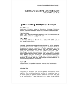
We used a typical property in the sample to illustrate the implications of
these results. The typical property has the following characteristics: B_SIZE
= 770, PARKING = 1.25, UNITS = 42, and U_PRICE = $38,900. Figure 2
illustrates the sensitivity of the NOI with respect to the R and C with the
estimated model. For a typical rental property in our sample, the optimal
strategy for rent and operating expense per unit are (R* , C*) = ($13,515,
$3,461). That is, the landlord should spend $3,461 to maintain each rental
unit, and the rental price should be $13,515 per unit. For this solution to be
an interior solution, Qd* must be smaller than the available quantity, 42
units. The quantity demanded is computed by substituting the estimated
parameters into Equation (9). This Qd* turns out to be 25 units, which is
smaller than 42 units, the size of the building. As a result, the physical
constraint is not binding. The optimal NOI is found to be $193,831 per
period. We found the operating ratios indicated by the strategy of
maximizing the net operating income:
V * = 40.25%,
*
IR = 34.15%, and
OER * = 42.85%.
We then compared the optimal R*, C*, V*, IR* and OER* with the actual
data on the individual property level. From Table 4, we found that the actual
operating expenses and the actual rents in most properties were lower than
the optimal solutions suggested by the model. Landlords could increase the
NOI by increasing the quality of the property by putting in more operating
expenses and simultaneously charging higher rents. Table 5 shows that the
actual income ratios tend to be too high, and the actual operating expense
18. 18 Colwell, Kung and Yang
ratios tend to be too low. Investors could increase profitability by increasing
operating expenses more relative to the amount of increases in rent.
Figure 2 Net Operating Income of a Typical Apartment in Southern
California
200,000
150,000
NOI ($)
100,000
50,000
4,000
Operating
- 0 Expense ($/unit)
10,000
13,000
16,000
19,000
22,000
1,000
4,000
7,000
Rent ($/unit)
NOI = g (R, C B_SIZE, PARKING, UNITS, U_PRICE)
B_SIZE = 770, PARKING = 1.25, UNITS = 42, and U_PRICE = 38,900.
Table 4 Comparison of R*, C* with R, C – Number of Properties
1.2 C* < C 0.8 C* < C < 1.2 C* C < 0.8 C*
*
1.2 R < R 2 2 0
0.8 R* < R < 1.2 R* 5 40 69
R < 0.8 R* 2 16 331
R and C are the actual rent and operating expenses of the property. R* an C* are the optimal
rent and operating expenses suggested by the model.
Table 5 Comparison of Operation Ratios – Number of Properties
1.3 X* < X 0.7 X* < X < 1.3 X* X < 0.7 X*
Vacancy Rate 101 174 192
Income Ratio 315 146 6
Operating 9 26 432
Expense Ratio
X represents the actual vacancy rate, income ratio, or operating expense ratio realized from the
property. X* represents the optimal level suggested by the model.
19. Optimal Property Management Strategies 19
One should notice that the sample represents a recession market. Southern
California suffered from a prolonged recession in the early 1990’s. The
vacancy rate during this time period tends to be high. Finding ways to attract
tenants is a very challenging task. The data observed in this empirical study
reflects this condition. However, our model suggests that there is significant
room for most property managers to improve their performance by resetting
their pricing strategies. Sometimes, higher income ratios and lower operating
expense ratios may not lead to maximum profitability.
Conclusions
In this paper, we showed that if the demand curve is time independent, then
investors in rental properties are expected to behave as if they are myopic.
That is, the strategy that maximizes the net present value of investment is
identical to maximizing a single period's net operating income.
With a given demand curve, one can algebraically derive the operating
strategies in terms of setting the levels of rent and operating expenses. We
used a Cobb-Douglas demand curve to demonstrate the process and to study
the properties of such optimal strategies. The impact of changes in market
conditions on NOI over time or across sub-markets care were also revealed
by comparative statics. These comparative statics also provided insights into
the adjustment that one can make corresponding to the new environment to
be maintained at the optimal position. These results also implied the ideal
building size under a specific market. Rehabilitation could be optimal as the
increase in the present value of net operating income exceeds the costs of
adjusting the building size.
Cross-sectional multi-family transaction data from southern California was
used to empirically estimate a Cobb-Douglas demand function. Based on the
estimated parameters, we found that the actual operating expense and the
actual rent tend to be lower than the optimal levels suggested by the model.
On the other hand, the income ratio tends to be too high and the operating
expense ratio tends to be too low. This suggests that when setting operating
strategies, property managers should not simply focus on one or two ratios.
Sensitivity of the demand (quantity) associated with the rent (price) and
operating expense (quality) are just as important.
This model can also be used when the demand curve is estimated by time
series data. With proprietary historical performance data, a property
manager would be able to determine the optimal operating strategy. This is
particularly valuable to managers of short-term lease properties, such as
hotels.
20. 20 Colwell, Kung and Yang
References
Cannaday, R. E. and Yang, T.L. Tyler, (1995), Optimal interest rate-discount
points combination: strategy for mortgage contract terms, Journal of the
American Real Estate and Urban Economics Association: Real Estate
Economics, 23, 1, 65-83.
Cannaday, R. E. and Yang, T.L. Tyler, (1996), Optimal Leverage Strategy:
Capital Structure in Real Estate Investments, Journal of Real Estate Finance
and Economics, 13, 3, 263-271.
Chinloy, Peter and Maribojoc, Eric, (1998), Expense and rent strategies in
real estate management, Journal of Real Estate Research, 15, 3, 267-282.
Colwell, Pete F., (1991), Vacancy management, Journal of Property
Management , 56, 3, 42-44.
Evans, Mariwyn, (1991), What is real estate worth?, A debate over the
meaning of market value, Journal of Property Management, 56, 3, 46-48.
21. Optimal Property Management Strategies 21
Appendix: Proof of the Comparative statics
Constraint Not Binding
1) Change of Q0 :
∂R * = (1 + β )(1 + δ )Q s > 0,
A
∂Q 0 ( β − δ )Q 0
∂C * = (1 + β )δ > 0,
A
∂Q 0 (β − δ )
∂NOI * =
A (1 + β )Q s > 0,
∂Q 0
∂V * = - β < 0,
∂Q 0
(1 + β )Q s
∂IR * = β − δ > 0,
∂Q 0 (1 + β )Q s
∂OER* = 0,
∂Q 0
1/(β-δ)
1+ δ
δ 0
δ Q
where A = > 0.
α (1 + β )1+ β Q s β
2) Change of Qs
∂R * = - A (1 + β )δ < 0,
∂Q s β −δ
∂C * = - A βδQ 0 < 0,
∂Q s ( β − δ )Q s
∂NOI * = - δ Q0 < 0,
A
∂Q s
∂V * = βQ 0 > 0,
∂Q s (1 + β )Q s
2
∂IR * = - ( β − δ )Q 0 < 0, and
∂Q s (1 + β )Q s
2
∂OER* = 0.
∂Q s
22. 22 Colwell, Kung and Yang
3) Change of α
∂R * = - (1 + β )Q s
A < 0,
∂α ( β − δ )α
∂C * = - δQ 0 < 0,
A
∂α ( β − δ )α
∂NOI * = - Q 0 Q s < 0,
A
∂α α
∂V * = 0,
∂α
∂IR *
= 0, and
∂α
∂OER* = 0.
∂α
4) Change of β
∂R * 1+ β
= A Qs
( β − δ ) 2 D + 1
,
∂β
∂C * δQ 0 D,
=A
∂β (β − δ )2
∂NOI * D
= A Q0 Qs
∂β β − δ + 2 ,
∂V * Q0
=- < 0,
∂β (1 + β ) 2 Q s
∂IR * (1 + δ )Q 0 > 0, and
=
∂β (1 + β ) 2 Q s
∂OER* = - δ < 0,
∂β β2
where D = log(α) + (1 + δ) log(1 + β) - δ log(δ) - (1 + δ) log(Q0) + δ
log(Qs) - (β - δ)