Fin 2 book

● ● ● ● ●
confirming pages
101
PART 1
◗ A company’s shareholders prefer to be rich
rather than poor. Therefore, they want the firm to invest
in every project that is worth more than it costs. The
difference between a project’s value and its cost is its
net present value (NPV). Companies can best help their
shareholders by investing in all projects with a positive
NPV and rejecting those with a negative NPV.
We start this chapter with a review of the net present
value rule. We then turn to some other measures that
companies may look at when making investment
decisions. The first two of these measures, the project’s
payback period and its book rate of return, are little
better than rules of thumb, easy to calculate and easy
to communicate. Although there is a place for rules
of thumb in this world, an engineer needs something
more accurate when designing a 100-story building,
and a financial manager needs more than a rule of
thumb when making a substantial capital investment
decision.
Instead of calculating a project’s NPV, companies
often compare the expected rate of return from investing
in the project with the return that shareholders could earn
on equivalent-risk investments in the capital market. The
company accepts those projects that provide a higher
return than shareholders could earn for themselves. If
used correctly, this rate of return rule should always
identify projects that increase firm value. However, we
shall see that the rule sets several traps for the unwary.
We conclude the chapter by showing how to cope
with situations when the firm has only limited capital.
This raises two problems. One is computational. In
simple cases we just choose those projects that give
the highest NPV per dollar invested, but more elaborate
techniques are sometimes needed to sort through the
possible alternatives. The other problem is to decide
whether capital rationing really exists and whether
it invalidates the net present value rule. Guess what?
NPV, properly interpreted, wins out in the end.
Net Present Value and
Other Investment Criteria
5CHAPTER
VALUE
● ● ● ● ●
Vegetron’s chief financial officer (CFO) is wondering how to analyze a proposed $1 million
investment in a new venture called project X. He asks what you think.
Your response should be as follows: “First, forecast the cash flows generated by project
X over its economic life. Second, determine the appropriate opportunity cost of capital (r).
This should reflect both the time value of money and the risk involved in project X. Third,
use this opportunity cost of capital to discount the project’s future cash flows. The sum of
the discounted cash flows is called present value (PV). Fourth, calculate net present value
(NPV) by subtracting the $1 million investment from PV. If we call the cash flows C0, C1,
and so on, then
NPV ϭ C0 ϩ
C1
1 ϩ r
ϩ
C2
11 ϩ r22
ϩ c
5-1 A Review of the Basics
bre30735_ch05_101-126.indd 101bre30735_ch05_101-126.indd 101 12/1/09 3:42:52 PM12/1/09 3:42:52 PM

confirming pages
102 Part One Value
We should invest in project X if its NPV is greater than zero.”
However, Vegetron’s CFO is unmoved by your sagacity. He asks why NPV is so
important.
Your reply: “Let us look at what is best for Vegetron stockholders. They want you to
make their Vegetron shares as valuable as possible.
“Right now Vegetron’s total market value (price per share times the number of shares
outstanding) is $10 million. That includes $1 million cash we can invest in project X. The
value of Vegetron’s other assets and opportunities must therefore be $9 million. We have to
decide whether it is better to keep the $1 million cash and reject project X or to spend the
cash and accept the project. Let us call the value of the new project PV. Then the choice is
as follows:
Market Value ($ millions)
Asset Reject Project X Accept Project X
Cash 1 0
Other assets 9 9
Project X 0 PV
10 9 ϩ PV
“Clearly project X is worthwhile if its present value, PV, is greater than $1 million, that is,
if net present value is positive.”
CFO: “How do I know that the PV of project X will actually show up in Vegetron’s
market value?”
Your reply: “Suppose we set up a new, independent firm X, whose only asset is project X.
What would be the market value of firm X?
“Investors would forecast the dividends that firm X would pay and discount those divi-
dends by the expected rate of return of securities having similar risks. We know that stock
prices are equal to the present value of forecasted dividends.
“Since project X is the only asset, the dividend payments we would expect firm X to
pay are exactly the cash flows we have forecasted for project X. Moreover, the rate inves-
tors would use to discount firm X’s dividends is exactly the rate we should use to discount
project X’s cash flows.
“I agree that firm X is entirely hypothetical. But if project X is accepted, investors hold-
ing Vegetron stock will really hold a portfolio of project X and the firm’s other assets. We
know the other assets are worth $9 million considered as a separate venture. Since asset
values add up, we can easily figure out the portfolio value once we calculate the value of
project X as a separate venture.
“By calculating the present value of project X, we are replicating the process by which
the common stock of firm X would be valued in capital markets.”
CFO: “The one thing I don’t understand is where the discount rate comes from.”
Your reply: “I agree that the discount rate is difficult to measure precisely. But it is easy
to see what we are trying to measure. The discount rate is the opportunity cost of invest-
ing in the project rather than in the capital market. In other words, instead of accepting a
project, the firm can always return the cash to the shareholders and let them invest it in
financial assets.
“You can see the trade-off (Figure 5.1). The opportunity cost of taking the project is
the return shareholders could have earned had they invested the funds on their own.
When we discount the project’s cash flows by the expected rate of return on finan-
cial assets, we are measuring how much investors would be prepared to pay for your
project.”

confirming pages
Chapter 5 Net Present Value and Other Investment Criteria 103
“But which financial assets?” Vegetron’s CFO queries. “The fact that investors expect
only 12% on IBM stock does not mean that we should purchase Fly-by-Night Electronics
if it offers 13%.”
Your reply: “The opportunity-cost concept makes sense only if assets of equivalent risk
are compared. In general, you should identify financial assets that have the same risk as
your project, estimate the expected rate of return on these assets, and use this rate as the
opportunity cost.”
Net Present Value’s Competitors
When you advised the CFO to calculate the project’s NPV, you were in good company.
These days 75% of firms always, or almost always, calculate net present value when decid-
ing on investment projects. However, as you can see from Figure 5.2, NPV is not the only
investment criterion that companies use, and firms often look at more than one measure
of a project’s attractiveness.
About three-quarters of firms calculate the project’s internal rate of return (or IRR); that
is roughly the same proportion as use NPV. The IRR rule is a close relative of NPV and,
when used properly, it will give the same answer. You therefore need to understand the IRR
rule and how to take care when using it.
A large part of this chapter is concerned with explaining the IRR rule, but first we look
at two other measures of a project’s attractiveness—the project’s payback and its book rate
of return. As we will explain, both measures have obvious defects. Few companies rely on
them to make their investment decisions, but they do use them as supplementary measures
that may help to distinguish the marginal project from the no-brainer.
Later in the chapter we also come across one further investment measure, the profit-
ability index. Figure 5.2 shows that it is not often used, but you will find that there are
circumstances in which this measure has some special advantages.
Three Points to Remember about NPV
As we look at these alternative criteria, it is worth keeping in mind the following key fea-
tures of the net present value rule. First, the NPV rule recognizes that a dollar today is
worth more than a dollar tomorrow, because the dollar today can be invested to start earning
interest immediately. Any investment rule that does not recognize the time value of money
cannot be sensible. Second, net present value depends solely on the forecasted cash flows
◗ FIGURE 5.1
The firm can either
keep and reinvest
cash or return it to
investors. (Arrows
represent possible cash
flows or transfers.)
If cash is reinvested,
the opportunity cost
is the expected rate of
return that shareholders
could have obtained by
investing in financial
assets.
Financial
manager
Invest
Shareholders
Cash
Investment
(project X)
Investment
(financial assets)
Alternative:
pay dividend
to shareholders
Shareholders
invest for themselves

confirming pages
104 Part One Value
from the project and the opportunity cost of capital. Any investment rule that is affected by
the manager’s tastes, the company’s choice of accounting method, the profitability of the
company’s existing business, or the profitability of other independent projects will lead to
inferior decisions. Third, because present values are all measured in today’s dollars, you can add
them up. Therefore, if you have two projects A and B, the net present value of the combined
investment is
NPV1A ϩ B2 ϭ NPV1A2 ϩ NPV1B2
This adding-up property has important implications. Suppose project B has a negative
NPV. If you tack it onto project A, the joint project (A ϩ B) must have a lower NPV than
A on its own. Therefore, you are unlikely to be misled into accepting a poor project (B) just
because it is packaged with a good one (A). As we shall see, the alternative measures do not
have this property. If you are not careful, you may be tricked into deciding that a package
of a good and a bad project is better than the good project on its own.
NPV Depends on Cash Flow, Not on Book Returns
Net present value depends only on the project’s cash flows and the opportunity cost of
capital. But when companies report to shareholders, they do not simply show the cash
flows. They also report book—that is, accounting—income and book assets.
Financial managers sometimes use these numbers to calculate a book (or accounting)
rate of return on a proposed investment. In other words, they look at the prospective
book income as a proportion of the book value of the assets that the firm is proposing to
acquire:
Book rate of return ϭ
book income
book assets
Cash flows and book income are often very different. For example, the accountant labels
some cash outflows as capital investments and others as operating expenses. The operating
expenses are, of course, deducted immediately from each year’s income. The capital
expenditures are put on the firm’s balance sheet and then depreciated. The annual depre-
ciation charge is deducted from each year’s income. Thus the book rate of return depends
◗ FIGURE 5.2
Survey evidence on the percentage of CFOs who always, or almost always, use a particular technique for
evaluating investment projects.
Source: Reprinted from J. R. Graham and C. R. Harvey, “The Theory and Practice of Finance: Evidence from the Field,” Journal of
Financial Economics 61 (2001), pp. 187–243, © 2001 with permission from Elsevier Science.
Profitability index:
12%
Book rate of return:
20%
Payback:
57%
IRR:
76%
NPV:
75%
%
40 10020 60 800

confirming pages
on which items the accountant treats as capital investments and how rapidly they are
depreciated.1
Now the merits of an investment project do not depend on how accountants classify
the cash flows2
and few companies these days make investment decisions just on the basis
of the book rate of return. But managers know that the company’s shareholders pay con-
siderable attention to book measures of profitability and naturally they think (and worry)
about how major projects would affect the company’s book return. Those projects that
would reduce the company’s book return may be scrutinized more carefully by senior
management.
You can see the dangers here. The company’s book rate of return may not be a good
measure of true profitability. It is also an average across all of the firm’s activities. The aver-
age profitability of past investments is not usually the right hurdle for new investments.
Think of a firm that has been exceptionally lucky and successful. Say its average book
return is 24%, double shareholders’ 12% opportunity cost of capital. Should it demand that
all new investments offer 24% or better? Clearly not: That would mean passing up many
positive-NPV opportunities with rates of return between 12 and 24%.
We will come back to the book rate of return in Chapters 12 and 28, when we look more
closely at accounting measures of financial performance.
We suspect that you have often heard conversations that go something like this: “We are
spending $6 a week, or around $300 a year, at the laundromat. If we bought a washing
machine for $800, it would pay for itself within three years. That’s well worth it.” You have
just encountered the payback rule.
A project’s payback period is found by counting the number of years it takes before
the cumulative cash flow equals the initial investment. For the washing machine the pay-
back period was just under three years. The payback rule states that a project should be
accepted if its payback period is less than some specified cutoff period. For example, if
the cutoff period is four years, the washing machine makes the grade; if the cutoff is two
years, it doesn’t.
EXAMPLE 5.1 ● The Payback Rule
Consider the following three projects:
Cash Flows ($)
Project C0 C1 C2 C3
Payback Period
(years) NPV at 10%
A Ϫ2,000 500 500 5,000 3 ϩ2,624
B Ϫ2,000 500 1,800 0 2 Ϫ58
C Ϫ2,000 1,800 500 0 2 ϩ50
1
This chapter’s mini-case contains simple illustrations of how book rates of return are calculated and of the difference between
accounting income and project cash flow. Read the case if you wish to refresh your understanding of these topics. Better still, do
the case calculations.
2
Of course, the depreciation method used for tax purposes does have cash consequences that should be taken into account in
calculating NPV. We cover depreciation and taxes in the next chapter.
5-2 Payback

confirming pages
106 Part One Value
Project A involves an initial investment of $2,000 (C0 ϭ Ϫ2,000) followed by cash inflows
during the next three years. Suppose the opportunity cost of capital is 10%. Then project
A has an NPV of ϩ$2,624:
NPV1A2 ϭ 22,000 ϩ
500
1.10
ϩ
500
1.102
ϩ
5,000
1.103
ϭ 1$2,624
Project B also requires an initial investment of $2,000 but produces a cash inflow of
$500 in year 1 and $1,800 in year 2. At a 10% opportunity cost of capital project B has an
NPV of Ϫ$58:
NPV1B2 ϭ 22,000 ϩ
500
1.10
ϩ
1,800
1.102
ϭ 2$58
The third project, C, involves the same initial outlay as the other two projects but its
first-period cash flow is larger. It has an NPV of ϩ$50.
NPV1C2 ϭ 22,000 ϩ
1,800
1.10
ϩ
500
1.102
ϭ 1$50
The net present value rule tells us to accept projects A and C but to reject project B.
Now look at how rapidly each project pays back its initial investment. With project A
you take three years to recover the $2,000 investment; with projects B and C you take only
two years. If the firm used the payback rule with a cutoff period of two years, it would accept
only projects B and C; if it used the payback rule with a cutoff period of three or more
years, it would accept all three projects. Therefore, regardless of the choice of cutoff period,
the payback rule gives different answers from the net present value rule.
You can see why payback can give misleading answers as illustrated in Example 5.1:
1. The payback rule ignores all cash flows after the cutoff date. If the cutoff date is two
years, the payback rule rejects project A regardless of the size of the cash inflow
in year 3.
2. The payback rule gives equal weight to all cash flows before the cutoff date. The payback rule
says that projects B and C are equally attractive, but because C’s cash inflows occur
earlier, C has the higher net present value at any discount rate.
In order to use the payback rule, a firm has to decide on an appropriate cutoff date. If it
uses the same cutoff regardless of project life, it will tend to accept many poor short-lived
projects and reject many good long-lived ones.
We have had little good to say about the payback rule. So why do many companies con-
tinue to use it? Senior managers don’t truly believe that all cash flows after the payback period
are irrelevant. We suggest three explanations. First, payback may be used because it is the sim-
plest way to communicate an idea of project profitability. Investment decisions require discus-
sion and negotiation between people from all parts of the firm, and it is important to have a
measure that everyone can understand. Second, managers of larger corporations may opt for
projects with short paybacks because they believe that quicker profits mean quicker promo-
tion. That takes us back to Chapter 1 where we discussed the need to align the objectives of
managers with those of shareholders. Finally, owners of family firms with limited access to
capital may worry about their future ability to raise capital. These worries may lead them to
favor rapid payback projects even though a longer-term venture may have a higher NPV.
● ● ● ● ●

confirming pages
Discounted Payback
Occasionally companies discount the cash flows before they compute the payback period.
The discounted cash flows for our three projects are as follows:
Discounted Cash Flows ($)
Project C0 C1 C2 C3
Discounted
Payback
Period (years)
NPV at
20%
A Ϫ2,000 500/1.10 ϭ
455
500/1.102
ϭ
413
5,000/1.103
ϭ
3,757
3 ϩ2,624
B Ϫ2,000 500/1.10 ϭ
455
1,800/1.102
ϭ
1,488
— Ϫ58
C Ϫ2,000 1,800/1.10 ϭ
1,636
500/1.102
ϭ
413
2 ϩ50
The discounted payback rule asks, How many years does the project have to last in order for it
to make sense in terms of net present value? You can see that the value of the cash inflows
from project B never exceeds the initial outlay and would always be rejected under the dis-
counted payback rule. Thus the discounted payback rule will never accept a negative-NPV
project. On the other hand, it still takes no account of cash flows after the cutoff date, so
that good long-term projects such as A continue to risk rejection.
Rather than automatically rejecting any project with a long discounted payback period,
many managers simply use the measure as a warning signal. These managers don’t unthink-
ingly reject a project with a long discounted-payback period. Instead they check that the
proposer is not unduly optimistic about the project’s ability to generate cash flows into the
distant future. They satisfy themselves that the equipment has a long life and that competi-
tors will not enter the market and eat into the project’s cash flows.
Whereas payback and return on book are ad hoc measures, internal rate of return has a
much more respectable ancestry and is recommended in many finance texts. If, therefore,
we dwell more on its deficiencies, it is not because they are more numerous but because
they are less obvious.
In Chapter 2 we noted that the net present value rule could also be expressed in terms
of rate of return, which would lead to the following rule: “Accept investment opportuni-
ties offering rates of return in excess of their opportunity costs of capital.” That statement,
properly interpreted, is absolutely correct. However, interpretation is not always easy for
long-lived investment projects.
There is no ambiguity in defining the true rate of return of an investment that generates
a single payoff after one period:
Rate of return ϭ
payoff
investment
Ϫ 1
Alternatively, we could write down the NPV of the investment and find the discount rate
that makes NPV ϭ 0.
NPV ϭ C0 ϩ
C1
1 ϩ discount rate
ϭ 0
5-3 Internal (or Discounted-Cash-Flow) Rate of Return

confirming pages
108 Part One Value
implies
Discount rate ϭ
C1
2C0
Ϫ 1
Of course C1 is the payoff and ϪC0 is the required investment, and so our two equations
say exactly the same thing. The discount rate that makes NPV ϭ 0 is also the rate of return.
How do we calculate return when the project produces cash flows in several periods?
Answer: we use the same definition that we just developed for one-period projects—the
project rate of return is the discount rate that gives a zero NPV. This discount rate is known as the
discounted-cash-flow (DCF) rate of return or internal rate of return (IRR). The internal
rate of return is used frequently in finance. It can be a handy measure, but, as we shall see,
it can also be a misleading measure. You should, therefore, know how to calculate it and
how to use it properly.
Calculating the IRR
The internal rate of return is defined as the rate of discount that makes NPV ϭ 0. So to find
the IRR for an investment project lasting T years, we must solve for IRR in the following
expression:
NPV ϭ C0 ϩ
C1
1 ϩ IRR
ϩ
C2
11 ϩ IRR22
ϩ cϩ
CT
11 ϩ IRR2T
ϭ 0
Actual calculation of IRR usually involves trial and error. For example, consider a proj-
ect that produces the following flows:
Cash Flows ($)
C0 C1 C2
Ϫ4,000 ϩ2,000 ϩ4,000
The internal rate of return is IRR in the equation
NPV ϭ 24,000 ϩ
2,000
1 ϩ IRR
ϩ
4,000
11 ϩ IRR22
ϭ 0
Let us arbitrarily try a zero discount rate. In this case NPV is not zero but ϩ$2,000:
NPV ϭ 24,000 ϩ
2,000
1.0
ϩ
4,000
11.022
ϭ 1$2,000
The NPV is positive; therefore, the IRR must be greater than zero. The next step might be
to try a discount rate of 50%. In this case net present value is Ϫ$889:
NPV ϭ 24,000 ϩ
2,000
1.50
ϩ
4,000
11.5022
ϭ 2$889
The NPV is negative; therefore, the IRR must be less than 50%. In Figure 5.3 we have
plotted the net present values implied by a range of discount rates. From this we can see
that a discount rate of 28% gives the desired net present value of zero. Therefore IRR
is 28%.
The easiest way to calculate IRR, if you have to do it by hand, is to plot three or four combi-
nations of NPV and discount rate on a graph like Figure 5.3, connect the points with a smooth
line, and read off the discount rate at which NPV ϭ 0. It is of course quicker and more accurate
to use a computer spreadsheet or a specially programmed calculator, and in practice this is what

confirming pages
financial managers do. The Useful
Spreadsheet Functions box near
the end of the chapter presents
Excel functions for doing so.
Some people confuse the inter-
nal rate of return and the opportu-
nity cost of capital because both
appear as discount rates in the NPV
formula. The internal rate of return
is a profitabilitymeasure that depends
solely on the amount and timing of
the project cash flows. The oppor-
tunity cost of capital is a standard
of profitability that we use to calcu-
late how much the project is worth.
The opportunity cost of capital is
established in capital markets. It is
the expected rate of return offered
by other assets with the same risk as
the project being evaluated.
The IRR Rule
The internal rate of return rule is to accept an investment project if the opportunity cost of
capital is less than the internal rate of return. You can see the reasoning behind this idea
if you look again at Figure 5.3. If the opportunity cost of capital is less than the 28%
IRR, then the project has a positive NPV when discounted at the opportunity cost of
capital. If it is equal to the IRR, the project has a zero NPV. And if it is greater than the
IRR, the project has a negative NPV. Therefore, when we compare the opportunity cost
of capital with the IRR on our project, we are effectively asking whether our project has
a positive NPV. This is true not only for our example. The rule will give the same answer
as the net present value rule whenever the NPV of a project is a smoothly declining function of
the discount rate.
Many firms use internal rate of return as a criterion in preference to net present value.
We think that this is a pity. Although, properly stated, the two criteria are formally equiva-
lent, the internal rate of return rule contains several pitfalls.
Pitfall 1—Lending or Borrowing?
Not all cash-flow streams have NPVs that decline as the discount rate increases. Consider
the following projects A and B:
Cash Flows ($)
Project C0 C1 IRR NPV at 10%
A Ϫ1,000 ϩ1,500 ϩ50% ϩ364
B ϩ1,000 Ϫ1,500 ϩ50% Ϫ364
Each project has an IRR of 50%. (In other words, Ϫ1,000 ϩ 1,500/1.50 ϭ 0 and ϩ 1,000
Ϫ 1,500/1.50 ϭ 0.)
Does this mean that they are equally attractive? Clearly not, for in the case of A, where
we are initially paying out $1,000, we are lending money at 50%, in the case of B, where we
–2,000
Net present value, dollars
Discount rate, %
+1,000
0
–1,000
+$2,000
1009080706050402010
IRR = 28%
◗ FIGURE 5.3
This project costs
$4,000 and then
produces cash inflows
of $2,000 in year 1 and
$4,000 in year 2. Its
internal rate of return
(IRR) is 28%, the rate of
discount at which NPV
is zero.

confirming pages
110 Part One Value
are initially receiving $1,000, we are borrowing money at 50%. When we lend money, we
want a high rate of return; when we borrow money, we want a low rate of return.
If you plot a graph like Figure 5.3 for project B, you will find that NPV increases as the
discount rate increases. Obviously the internal rate of return rule, as we stated it above, won’t
work in this case; we have to look for an IRR less than the opportunity cost of capital.
Pitfall 2—Multiple Rates of Return
Helmsley Iron is proposing to develop a new strip mine in Western Australia. The mine
involves an initial investment of A$3 billion and is expected to produce a cash inflow of
A$1 billion a year for the next nine years. At the end of that time the company will incur
A$6.5 billion of cleanup costs. Thus the cash flows from the project are:
Cash Flows (billions of Australian dollars)
C0 C1 . . . C9 C10
Ϫ3 1 1 Ϫ6.5
Helmsley calculates the project’s IRR and its NPV as follows:
IRR (%) NPV at 10%
ϩ3.50 and 19.54 $A253 million
Note that there are two discount rates that make NPV ϭ 0. That is, each of the following
statements holds:
NPV ϭ 23 ϩ
1
1.035
ϩ
1
1.0352
ϩ cϩ
1
1.0359
Ϫ
6.5
1.03510
ϭ 0
NPV ϭ 23 ϩ
1
1.1954
ϩ
1
1.19542
ϩ cϩ
1
1.19549
Ϫ
6.5
1.195410
ϭ 0
In other words, the investment has an IRR of both 3.50 and 19.54%. Figure 5.4 shows how
this comes about. As the discount rate increases, NPV initially rises and then declines. The
reason for this is the double change in the sign of the cash-flow stream. There can be as many
internal rates of return for a project as there are changes in the sign of the cash flows.3
Decommissioning and clean-up costs can sometimes be huge. Phillips Petroleum has
estimated that it will need to spend $1 billion to remove its Norwegian offshore oil plat-
forms. It can cost over $300 million to decommission a nuclear power plant. These are
obvious instances where cash flows go from positive to negative, but you can probably
think of a number of other cases where the company needs to plan for later expenditures.
Ships periodically need to go into dry dock for a refit, hotels may receive a major face-lift,
machine parts may need replacement, and so on.
Whenever the cash-flow stream is expected to change sign more than once, the company
typically sees more than one IRR.
As if this is not difficult enough, there are also cases in which no internal rate of return
exists. For example, project C has a positive net present value at all discount rates:
Cash Flows ($)
Project C0 C1 C2 IRR (%) NPV at 10%
C ϩ1,000 Ϫ3,000 ϩ2,500 None ϩ339
3
By Descartes’s “rule of signs” there can be as many different solutions to a polynomial as there are changes of sign.

confirming pages
A number of adaptations of the IRR rule have been devised for such cases. Not only are they
inadequate, but they also are unnecessary, for the simple solution is to use net present value.4
Pitfall 3—Mutually Exclusive Projects
Firms often have to choose from among several alternative ways of doing the same job or
using the same facility. In other words, they need to choose from among mutually exclu-
sive projects. Here too the IRR rule can be misleading.
Consider projects D and E:
Cash Flows ($)
Project C0 C1 IRR (%) NPV at 10%
D Ϫ10,000 ϩ20,000 100 ϩ 8,182
E Ϫ20,000 ϩ35,000 75 ϩ11,818
Perhaps project D is a manually controlled machine tool and project E is the same tool with
the addition of computer control. Both are good investments, but E has the higher NPV and
is, therefore, better. However, the IRR rule seems to indicate that if you have to choose, you
should go for D since it has the higher IRR. If you follow the IRR rule, you have the satisfac-
tion of earning a 100% rate of return; if you follow the NPV rule, you are $11,818 richer.
4
Companies sometimes get around the problem of multiple rates of return by discounting the later cash flows back at the cost
of capital until there remains only one change in the sign of the cash flows. A modified internal rate of return (MIRR) can then be
calculated on this revised series. In our example, the MIRR is calculated as follows:
1. Calculate the present value in year 5 of all the subsequent cash flows:
PV in year 5 = 1/1.1 ϩ 1/1.12
ϩ 1/1.13
ϩ ϩ1/1.14
Ϫ 6.5/1.15
ϭ Ϫ.866
2. Add to the year 5 cash flow the present value of subsequent cash flows:
C5 ϩ PV(subsequent cash flows) ϭ 1 Ϫ.866 ϭ .134
3. Since there is now only one change in the sign of the cash flows, the revised series has a unique rate of return, which is
13.7%
NPV ϭ 1/1.137 ϩ 1/1.1372
ϩ 1/1.1373
ϩ 1/1.1374
ϩ .134/1.1375
ϭ 0
Since the MIRR of 13.7% is greater than the cost of capital (and the initial cash flow is negative), the project has a positive NPV
when valued at the cost of capital.
Of course, it would be much easier in such cases to abandon the IRR rule and just calculate project NPV.
◗ FIGURE 5.4
Helmsley Iron’s mine has two internal rates of return. NPV ϭ 0 when the discount rate is ϩ3.50% and when it is ϩ19.54%.
NPV, A$billions
Discount rate, %
+40
0
–60
0 5 10 15 20 25 30 35
IRR = 19.54%IRR = 3.50%
–80
–20
–40
+20

confirming pages
112 Part One Value
You can salvage the IRR rule in these cases by looking at the internal rate of return on
the incremental flows. Here is how to do it: First, consider the smaller project (D in our
example). It has an IRR of 100%, which is well in excess of the 10% opportunity cost of
capital. You know, therefore, that D is acceptable. You now ask yourself whether it is worth
making the additional $10,000 investment in E. The incremental flows from undertaking E
rather than D are as follows:
Cash Flows ($)
Project C0 C1 IRR (%) NPV at 10%
E Ϫ D Ϫ10,000 ϩ15,000 50 ϩ3,636
The IRR on the incremental investment is 50%, which is also well in excess of the 10%
opportunity cost of capital. So you should prefer project E to project D.5
Unless you look at the incremental expenditure, IRR is unreliable in ranking projects of
different scale. It is also unreliable in ranking projects that offer different patterns of cash
flow over time. For example, suppose the firm can take project F or project G but not both
(ignore H for the moment):
Cash Flows ($)
Project C0 C1 C2 C3 C4 C5 Etc. IRR (%) NPV at 10%
F Ϫ9,000 ϩ6,000 ϩ5,000 ϩ4,000 0 0 . . . 33 3,592
G Ϫ9,000 ϩ1,800 ϩ1,800 ϩ1,800 ϩ1,800 ϩ1,800 . . . 20 9,000
H Ϫ6,000 ϩ1,200 ϩ1,200 ϩ1,200 ϩ1,200 . . . 20 6,000
Project F has a higher IRR, but project G, which is a perpetuity, has the higher NPV.
Figure 5.5 shows why the two rules give different answers. The green line gives the net pres-
ent value of project F at different rates of discount. Since a discount rate of 33% produces a
net present value of zero, this is the internal rate of return for project F. Similarly, the brown
line shows the net present value of project G at different discount rates. The IRR of project
G is 20%. (We assume project G’s cash flows continue indefinitely.) Note, however, that
project G has a higher NPV as long as the opportunity cost of capital is less than 15.6%.
The reason that IRR is misleading is that the total cash inflow of project G is larger but
tends to occur later. Therefore, when the discount rate is low, G has the higher NPV; when
the discount rate is high, F has the
higher NPV. (You can see from
Figure 5.5 that the two projects
have the same NPV when the dis-
count rate is 15.6%.) The internal
rates of return on the two projects
tell us that at a discount rate of 20%
G has a zero NPV (IRR ϭ 20%)
and F has a positive NPV. Thus
if the opportunity cost of capital
were 20%, investors would place a
higher value on the shorter-lived
project F. But in our example the
opportunity cost of capital is not
20% but 10%. So investors will
5
You may, however, find that you have jumped out of the frying pan into the fire. The series of incremental cash flows may involve
several changes in sign. In this case there are likely to be multiple IRRs and you will be forced to use the NPV rule after all.
–5,000
Net present value, dollars
Discount rate, %
Project F
Project G
+5,000
0
5040
3020
15.6%
33.3%
10
+6,000
+$10,000
◗ FIGURE 5.5
The IRR of project F
exceeds that of project
G, but the NPV of project
F is higher only if the
discount rate is greater
than 15.6%.

confirming pages
pay a relatively high price for the longer-lived project. At a 10% cost of capital, an investment
in G has an NPV of $9,000 and an investment in F has an NPV of only $3,592.6
This is a favorite example of ours. We have gotten many businesspeople’s reaction to
it. When asked to choose between F and G, many choose F. The reason seems to be the
rapid payback generated by project F. In other words, they believe that if they take F, they
will also be able to take a later project like H (note that H can be financed using the cash
flows from F), whereas if they take G, they won’t have money enough for H. In other words
they implicitly assume that it is a shortage of capital that forces the choice between F and G.
When this implicit assumption is brought out, they usually admit that G is better if there
is no capital shortage.
But the introduction of capital constraints raises two further questions. The first stems
from the fact that most of the executives preferring F to G work for firms that would have
no difficulty raising more capital. Why would a manager at IBM, say, choose F on the
grounds of limited capital? IBM can raise plenty of capital and can take project H regard-
less of whether F or G is chosen; therefore H should not affect the choice between F and
G. The answer seems to be that large firms usually impose capital budgets on divisions and
subdivisions as a part of the firm’s planning and control system. Since the system is com-
plicated and cumbersome, the budgets are not easily altered, and so they are perceived as
real constraints by middle management.
The second question is this. If there is a capital constraint, either real or self-imposed,
should IRR be used to rank projects? The answer is no. The problem in this case is to find
the package of investment projects that satisfies the capital constraint and has the larg-
est net present value. The IRR rule will not identify this package. As we will show in the
next section, the only practical and general way to do so is to use the technique of linear
programming.
When we have to choose between projects F and G, it is easiest to compare the net pres-
ent values. But if your heart is set on the IRR rule, you can use it as long as you look at the
internal rate of return on the incremental flows. The procedure is exactly the same as we
showed above. First, you check that project F has a satisfactory IRR. Then you look at the
return on the incremental cash flows from G.
Cash Flows ($)
Project C0 C1 C2 C3 C4 C5 Etc. IRR (%) NPV at 10%
G Ϫ F 0 Ϫ4,200 Ϫ3,200 Ϫ2,200 ϩ1,800 ϩ1,800 . . . 15.6 ϩ5,408
The IRR on the incremental cash flows from G is 15.6%. Since this is greater than the
opportunity cost of capital, you should undertake G rather than F.7
Pitfall 4—What Happens When There Is More than
One Opportunity Cost of Capital?
We have simplified our discussion of capital budgeting by assuming that the opportunity
cost of capital is the same for all the cash flows, C1, C2, C3, etc. Remember our most general
formula for calculating net present value:
NPV ϭ C0 ϩ
C1
1 ϩ r1
ϩ
C2
11 ϩ r2 22
ϩ
C3
11 ϩ r3 23
ϩ c
6
It is often suggested that the choice between the net present value rule and the internal rate of return rule should depend on the
probable reinvestment rate. This is wrong. The prospective return on another independent investment should never be allowed to
influence the investment decision.
7
Because F and G had the same 10% cost of capital, we could choose between the two projects by asking whether the IRR on the
incremental cash flows was greater or less than 10%. But suppose that F and G had different risks and therefore different costs of
capital. In that case there would be no simple yardstick for assessing whether the IRR on the incremental cash flows was adequate.

confirming pages
114 Part One Value
In other words, we discount C1 at the opportunity cost of capital for one year, C2 at the
opportunity cost of capital for two years, and so on. The IRR rule tells us to accept a proj-
ect if the IRR is greater than the opportunity cost of capital. But what do we do when we
have several opportunity costs? Do we compare IRR with r1, r2, r3, . . .? Actually we would
have to compute a complex weighted average of these rates to obtain a number comparable
to IRR.
What does this mean for capital budgeting? It means trouble for the IRR rule whenever
there is more than one opportunity cost of capital. Many firms use the IRR, thereby implic-
itly assuming that there is no difference between short-term and long-term discount rates.
They do this for the same reason that we have so far finessed the issue: simplicity.8
The Verdict on IRR
We have given four examples of things that can go wrong with IRR. We spent much less
space on payback or return on book. Does this mean that IRR is worse than the other
two measures? Quite the contrary. There is little point in dwelling on the deficiencies of
payback or return on book. They are clearly ad hoc measures that often lead to silly conclu-
sions. The IRR rule has a much more respectable ancestry. It is less easy to use than NPV,
but, used properly, it gives the same answer.
Nowadays few large corporations use the payback period or return on book as their
primary measure of project attractiveness. Most use discounted cash flow or “DCF,” and
for many companies DCF means IRR, not NPV. For “normal” investment projects with
an initial cash outflow followed by a series of cash inflows, there is no difficulty in using
the internal rate of return to make a simple accept/reject decision. However, we think that
financial managers need to worry more about Pitfall 3. Financial managers never see all pos-
sible projects. Most projects are proposed by operating managers. A company that instructs
nonfinancial managers to look first at project IRRs prompts a search for those projects
with the highest IRRs rather than the highest NPVs. It also encourages managers to modify
projects so that their IRRs are higher. Where do you typically find the highest IRRs? In
short-lived projects requiring little up-front investment. Such projects may not add much
to the value of the firm.
We don’t know why so many companies pay such close attention to the internal rate
of return, but we suspect that it may reflect the fact that management does not trust the
forecasts it receives. Suppose that two plant managers approach you with proposals for
two new investments. Both have a positive NPV of $1,400 at the company’s 8% cost
of capital, but you nevertheless decide to accept project A and reject B. Are you being
irrational?
The cash flows for the two projects and their NPVs are set out in the table below. You
can see that, although both proposals have the same NPV, project A involves an investment
of $9,000, while B requires an investment of $9 million. Investing $9,000 to make $1,400
is clearly an attractive proposition, and this shows up in A’s IRR of nearly 16%. Investing
$9 million to make $1,400 might also be worth doing if you could be sure of the plant
manager’s forecasts, but there is almost no room for error in project B. You could spend
time and money checking the cash-flow forecasts, but is it really worth the effort? Most
managers would look at the IRR and decide that, if the cost of capital is 8%, a project that
offers a return of 8.01% is not worth the worrying time.
Alternatively, management may conclude that project A is a clear winner that is worth
undertaking right away, but in the case of project B it may make sense to wait and see
8
In Chapter 9 we look at some other cases in which it would be misleading to use the same discount rate for both short-term and
long-term cash flows.

confirming pages
whether the decision looks more clear-cut in a year’s time.9
Management postpones the
decision on projects such as B by setting a hurdle rate for the IRR that is higher than the
cost of capital.
Cash Flows ($ thousands)
Project C0 C1 C2 C3 NPV at 8% IRR (%)
A Ϫ9.0 2.9 4.0 5.4 1.4 15.58
B Ϫ9,000 2,560 3,540 4,530 1.4 8.01
Our entire discussion of methods of capital budgeting has rested on the proposition that
the wealth of a firm’s shareholders is highest if the firm accepts every project that has a
positive net present value. Suppose, however, that there are limitations on the investment
program that prevent the company from undertaking all such projects. Economists call
this capital rationing. When capital is rationed, we need a method of selecting the pack-
age of projects that is within the company’s resources yet gives the highest possible net
present value.
An Easy Problem in Capital Rationing
Let us start with a simple example. The opportunity cost of capital is 10%, and our com-
pany has the following opportunities:
Cash Flows ($ millions)
Project C0 C1 C2 NPV at 10%
A Ϫ10 ϩ30 ϩ5 21
B Ϫ5 ϩ5 ϩ20 16
C Ϫ5 ϩ5 ϩ15 12
All three projects are attractive, but suppose that the firm is limited to spending
$10 million. In that case, it can invest either in project A or in projects B and C, but it can-
not invest in all three. Although individually B and C have lower net present values than
project A, when taken together they have the higher net present value. Here we cannot
choose between projects solely on the basis of net present values. When funds are limited,
we need to concentrate on getting the biggest bang for our buck. In other words, we must
pick the projects that offer the highest net present value per dollar of initial outlay. This
ratio is known as the profitability index:10
Profitability index ϭ
net present value
investment
9
In Chapter 22 we discuss when it may pay a company to delay undertaking a positive-NPV project. We will see that when projects
are “deep-in-the-money” (project A), it generally pays to invest right away and capture the cash flows. However, in the case of
projects that are close-to-the-money (project B) it makes more sense to wait and see.
10
If a project requires outlays in two or more periods, the denominator should be the present value of the outlays. A few com-
panies do not discount the benefits or costs before calculating the profitability index. The less said about these companies the
better.
5-4 Choosing Capital Investments When Resources Are Limited

confirming pages
116 Part One Value
For our three projects the profitability index is calculated as follows:11
Project
Investment
($ millions)
NPV
($ millions)
Profitability
Index
A 10 21 2.1
B 5 16 3.2
C 5 12 2.4
Project B has the highest profitability index and C has the next highest. Therefore, if our
budget limit is $10 million, we should accept these two projects.12
Unfortunately, there are some limitations to this simple ranking method. One of the
most serious is that it breaks down whenever more than one resource is rationed.13
For exam-
ple, suppose that the firm can raise only $10 million for investment in each of years 0 and
1 and that the menu of possible projects is expanded to include an investment next year in
project D:
Cash Flows ($ millions)
Project C0 C1 C2 NPV at 10% Profitability Index
A Ϫ10 ϩ30 ϩ5 21 2.1
B Ϫ5 ϩ5 ϩ20 16 3.2
C Ϫ5 ϩ5 ϩ15 12 2.4
D 0 Ϫ40 ϩ60 13 0.4
One strategy is to accept projects B and C; however, if we do this, we cannot also
accept D, which costs more than our budget limit for period 1. An alternative is to
accept project A in period 0. Although this has a lower net present value than the com-
bination of B and C, it provides a $30 million positive cash flow in period 1. When this
is added to the $10 million budget, we can also afford to undertake D next year. A and
D have lower profitability indexes than B and C, but they have a higher total net present
value.
The reason that ranking on the profitability index fails in this example is that resources
are constrained in each of two periods. In fact, this ranking method is inadequate whenever
there is any other constraint on the choice of projects. This means that it cannot cope with
cases in which two projects are mutually exclusive or in which one project is dependent on
another.
For example, suppose that you have a long menu of possible projects starting this year
and next. There is a limit on how much you can invest in each year. Perhaps also you can’t
undertake both project alpha and beta (they both require the same piece of land), and you
can’t invest in project gamma unless you invest in delta (gamma is simply an add-on to
11
Sometimes the profitability index is defined as the ratio of the present value to initial outlay, that is, as PV/investment. This
measure is also known as the benefit–cost ratio. To calculate the benefit–cost ratio, simply add 1.0 to each profitability index. Project
rankings are unchanged.
12
If a project has a positive profitability index, it must also have a positive NPV. Therefore, firms sometimes use the profitability
index to select projects when capital is not limited. However, like the IRR, the profitability index can be misleading when used
to choose between mutually exclusive projects. For example, suppose you were forced to choose between (1) investing $100 in a
project whose payoffs have a present value of $200 or (2) investing $1 million in a project whose payoffs have a present value of
$1.5 million. The first investment has the higher profitability index; the second makes you richer.
13
It may also break down if it causes some money to be left over. It might be better to spend all the available funds even if this
involves accepting a project with a slightly lower profitability index.

confirming pages
delta). You need to find the package of projects that satisfies all these constraints and gives
the highest NPV.
One way to tackle such a problem is to work through all possible combinations of
projects. For each combination you first check whether the projects satisfy the con-
straints and then calculate the net present value. But it is smarter to recognize that linear
programming (LP) techniques are specially designed to search through such possible
combinations.14
Uses of Capital Rationing Models
Linear programming models seem tailor-made for solving capital budgeting problems
when resources are limited. Why then are they not universally accepted either in theory
or in practice? One reason is that these models can turn out to be very complex. Sec-
ond, as with any sophisticated long-range planning tool, there is the general problem of
getting good data. It is just not worth applying costly, sophisticated methods to poor
data. Furthermore, these models are based on the assumption that all future investment
opportunities are known. In reality, the discovery of investment ideas is an unfolding
process.
Our most serious misgivings center on the basic assumption that capital is limited.
When we come to discuss company financing, we shall see that most large corporations do
not face capital rationing and can raise large sums of money on fair terms. Why then do
many company presidents tell their subordinates that capital is limited? If they are right,
the capital market is seriously imperfect. What then are they doing maximizing NPV?15
We
might be tempted to suppose that if capital is not rationed, they do not need to use linear
programming and, if it is rationed, then surely they ought not to use it. But that would be
too quick a judgment. Let us look at this problem more deliberately.
Soft Rationing Many firms’ capital constraints are “soft.” They reflect no imperfections
in capital markets. Instead they are provisional limits adopted by management as an aid to
financial control.
Some ambitious divisional managers habitually overstate their investment opportuni-
ties. Rather than trying to distinguish which projects really are worthwhile, headquarters
may find it simpler to impose an upper limit on divisional expenditures and thereby force
the divisions to set their own priorities. In such instances budget limits are a rough but
effective way of dealing with biased cash-flow forecasts. In other cases management may
believe that very rapid corporate growth could impose intolerable strains on management
and the organization. Since it is difficult to quantify such constraints explicitly, the budget
limit may be used as a proxy.
Because such budget limits have nothing to do with any inefficiency in the capital
market, there is no contradiction in using an LP model in the division to maximize net
present value subject to the budget constraint. On the other hand, there is not much point
in elaborate selection procedures if the cash-flow forecasts of the division are seriously
biased.
Even if capital is not rationed, other resources may be. The availability of management
time, skilled labor, or even other capital equipment often constitutes an important con-
straint on a company’s growth.
14
On our Web site at www.mhhe.com/bma we show how linear programming can be used to select from the four projects in our
earlier example.
15
Don’t forget that in Chapter 1 we had to assume perfect capital markets to derive the NPV rule.

● ● ● ● ●
confirming pages
118
◗ Spreadsheet programs such as Excel provide built-in
functions to solve for internal rates of return. You can
find these functions by pressing fx on the Excel toolbar.
If you then click on the function that you wish to use,
Excel will guide you through the inputs that are required.
At the bottom left of the function box there is a Help
facility with an example of how the function is used.
Here is a list of useful functions for calculating
internal rates of return, together with some points to
remember when entering data:
• IRR: Internal rate of return on a series of
regularly spaced cash flows.
• XIRR: The same as IRR, but for irregularly
spaced flows.
Note the following:
• For these functions, you must enter the addresses
of the cells that contain the input values.
• The IRR functions calculate only one IRR even
when there are multiple IRRs.
SPREADSHEET QUESTIONS
The following questions provide an opportunity to
practice each of the above functions:
1. (IRR) Check the IRRs on projects F and G in
Section 5-3.
2. (IRR) What is the IRR of a project with the fol-
lowing cash flows:
C0 C1 C2 C3
Ϫ$5,000 ϩ$2,200 ϩ$4,650 ϩ$3,330
3. (IRR) Now use the function to calculate the IRR
on Helmsley Iron’s mining project in Section 5-3.
There are really two IRRs to this project (why?).
How many IRRs does the function calculate?
4. (XIRR) What is the IRR of a project with the fol-
lowing cash flows:
C0 C4 C5 C6
Ϫ$215,000 . . . ϩ$185,000 . . . ϩ$85,000 . . . ϩ$43,000
(All other cash flows are 0.)
Internal Rate of Return
USEFUL SPREADSHEET FUNCTIONS
Hard Rationing Soft rationing should never cost the firm anything. If capital constraints
become tight enough to hurt—in the sense that projects with significant positive NPVs are
passed up—then the firm raises more money and loosens the constraint. But what if it can’t
raise more money—what if it faces hard rationing?
Hard rationing implies market imperfections, but that does not necessarily mean we
have to throw away net present value as a criterion for capital budgeting. It depends on the
nature of the imperfection.
Arizona Aquaculture, Inc. (AAI), borrows as much as the banks will lend it, yet it still has
good investment opportunities. This is not hard rationing so long as AAI can issue stock.
But perhaps it can’t. Perhaps the founder and majority shareholder vetoes the idea from

Visitusatwww.mhhe.com/bma
confirming pages
fear of losing control of the firm. Perhaps a stock issue would bring costly red tape or legal
complications.16
This does not invalidate the NPV rule. AAI’s shareholders can borrow or lend, sell their
shares, or buy more. They have free access to security markets. The type of portfolio they
hold is independent of AAI’s financing or investment decisions. The only way AAI can
help its shareholders is to make them richer. Thus AAI should invest its available cash in
the package of projects having the largest aggregate net present value.
A barrier between the firm and capital markets does not undermine net present value so
long as the barrier is the only market imperfection. The important thing is that the firm’s
shareholders have free access to well-functioning capital markets.
The net present value rule is undermined when imperfections restrict shareholders’ port-
folio choice. Suppose that Nevada Aquaculture, Inc. (NAI), is solely owned by its founder,
Alexander Turbot. Mr. Turbot has no cash or credit remaining, but he is convinced that
expansion of his operation is a high-NPV investment. He has tried to sell stock but has
found that prospective investors, skeptical of prospects for fish farming in the desert, offer
him much less than he thinks his firm is worth. For Mr. Turbot capital markets hardly exist.
It makes little sense for him to discount prospective cash flows at a market opportunity
cost of capital.
16
A majority owner who is “locked in” and has much personal wealth tied up in AAI may be effectively cut off from capital mar-
kets. The NPV rule may not make sense to such an owner, though it will to the other shareholders.
If you are going to persuade your company to use the net present value rule, you must be pre-
pared to explain why other rules may not lead to correct decisions. That is why we have exam-
ined three alternative investment criteria in this chapter.
Some firms look at the book rate of return on the project. In this case the company decides
which cash payments are capital expenditures and picks the appropriate rate to depreciate these
expenditures. It then calculates the ratio of book income to the book value of the investment.
Few companies nowadays base their investment decision simply on the book rate of return, but
shareholders pay attention to book measures of firm profitability and some managers therefore
look with a jaundiced eye on projects that would damage the company’s book rate of return.
Some companies use the payback method to make investment decisions. In other words,
they accept only those projects that recover their initial investment within some specified
period. Payback is an ad hoc rule. It ignores the timing of cash flows within the payback period,
and it ignores subsequent cash flows entirely. It therefore takes no account of the opportunity
cost of capital.
The internal rate of return (IRR) is defined as the rate of discount at which a project
would have zero NPV. It is a handy measure and widely used in finance; you should
therefore know how to calculate it. The IRR rule states that companies should accept any
investment offering an IRR in excess of the opportunity cost of capital. The IRR rule is,
like net present value, a technique based on discounted cash flows. It will therefore give the
correct answer if properly used. The problem is that it is easily misapplied. There are four
things to look out for:
1. Lending or borrowing? If a project offers positive cash flows followed by negative flows, NPV
can rise as the discount rate is increased. You should accept such projects if their IRR is less
than the opportunity cost of capital.
SUMMARY
● ● ● ● ●

confirming pages
120 Part One Value
2. Multiple rates of return. If there is more than one change in the sign of the cash flows, the
project may have several IRRs or no IRR at all.
3. Mutually exclusive projects. The IRR rule may give the wrong ranking of mutually exclusive
projects that differ in economic life or in scale of required investment. If you insist on using
IRR to rank mutually exclusive projects, you must examine the IRR on each incremental
investment.
4. The cost of capital for near-term cash flows may be different from the cost for distant cash flows. The
IRR rule requires you to compare the project’s IRR with the opportunity cost of capital. But
sometimes there is an opportunity cost of capital for one-year cash flows, a different cost
of capital for two-year cash flows, and so on. In these cases there is no simple yardstick for
evaluating the IRR of a project.
In developing the NPV rule, we assumed that the company can maximize shareholder
wealth by accepting every project that is worth more than it costs. But, if capital is strictly
limited, then it may not be possible to take every project with a positive NPV. If capital
is rationed in only one period, then the firm should follow a simple rule: Calculate each
project’s profitability index, which is the project’s net present value per dollar of invest-
ment. Then pick the projects with the highest profitability indexes until you run out of
capital. Unfortunately, this procedure fails when capital is rationed in more than one period
or when there are other constraints on project choice. The only general solution is linear
programming.
Hard capital rationing always reflects a market imperfection—a barrier between the firm and
capital markets. If that barrier also implies that the firm’s shareholders lack free access to a well-
functioning capital market, the very foundations of net present value crumble. Fortunately,
hard rationing is rare for corporations in the United States. Many firms do use soft capital
rationing, however. That is, they set up self-imposed limits as a means of financial planning
and control.
● ● ● ● ●
● ● ● ● ●
For a survey of capital budgeting procedures, see:
J. Graham and C. Harvey, “How CFOs Make Capital Budgeting and Capital Structure Deci-
sions,” Journal of Applied Corporate Finance 15 (spring 2002), pp. 8–23.
FURTHER
READING
Select problems are available in McGraw-Hill Connect.
Please see the preface for more information.
BASIC
1. a. What is the payback period on each of the following projects?
Cash Flows ($)
Project C0 C1 C2 C3 C4
A Ϫ5,000 ϩ1,000 ϩ1,000 ϩ3,000 0
B Ϫ1,000 0 ϩ1,000 ϩ2,000 ϩ3,000
C Ϫ5,000 ϩ1,000 ϩ1,000 ϩ3,000 ϩ5,000
PROBLEM SETS

confirming pages
b. Given that you wish to use the payback rule with a cutoff period of two years, which
projects would you accept?
c. If you use a cutoff period of three years, which projects would you accept?
d. If the opportunity cost of capital is 10%, which projects have positive NPVs?
e. “If a firm uses a single cutoff period for all projects, it is likely to accept too many short-
lived projects.” True or false?
f. If the firm uses the discounted-payback rule, will it accept any negative-NPV projects?
Will it turn down positive-NPV projects? Explain.
2. Write down the equation defining a project’s internal rate of return (IRR). In practice how
is IRR calculated?
3. a. Calculate the net present value of the following project for discount rates of 0, 50, and
100%:
Cash Flows ($)
C0 C1 C2
Ϫ6,750 ϩ4,500 ϩ18,000
b. What is the IRR of the project?
4. You have the chance to participate in a project that produces the following cash flows:
Cash Flows ($)
C0 C1 C2
ϩ5,000 ϩ4,000 Ϫ11,000
The internal rate of return is 13%. If the opportunity cost of capital is 10%, would you
accept the offer?
5. Consider a project with the following cash flows:
C0 C1 C2
Ϫ100 ϩ200 Ϫ75
a. How many internal rates of return does this project have?
b. Which of the following numbers is the project IRR:
(i) Ϫ50%; (ii) Ϫ12%; (iii) ϩ5%; (iv) ϩ50%?
c. The opportunity cost of capital is 20%. Is this an attractive project? Briefly explain.
6. Consider projects Alpha and Beta:
Cash Flows ($)
Project C0 C1 C2 IRR (%)
Alpha Ϫ400,000 ϩ241,000 ϩ293,000 21
Beta Ϫ200,000 ϩ131,000 ϩ172,000 31
The opportunity cost of capital is 8%.
Suppose you can undertake Alpha or Beta, but not both. Use the IRR rule to make the
choice. (Hint: What’s the incremental investment in Alpha?)

Rev.confirming Pages
122 Part One Value
7. Suppose you have the following investment opportunities, but only $90,000 available for
investment. Which projects should you take?
Project NPV Investment
1 5,000 10,000
2 5,000 5,000
3 10,000 90,000
4 15,000 60,000
5 15,000 75,000
6 3,000 15,000
INTERMEDIATE
8. Consider the following projects:
Cash Flows ($)
Project C0 C1 C2 C3 C4 C5
A Ϫ1,000 ϩ1,000 0 0 0 0
B Ϫ2,000 ϩ1,000 ϩ1,000 ϩ4,000 ϩ1,000 ϩ1,000
C Ϫ3,000 ϩ1,000 ϩ1,000 0 ϩ1,000 ϩ1,000
a. If the opportunity cost of capital is 10%, which projects have a positive NPV?
b. Calculate the payback period for each project.
c. Which project(s) would a firm using the payback rule accept if the cutoff period were
three years?
d. Calculate the discounted payback period for each project.
e. Which project(s) would a firm using the discounted payback rule accept if the cutoff
period were three years?
9. Respond to the following comments:
a. “I like the IRR rule. I can use it to rank projects without having to specify a discount rate.”
b. “I like the payback rule. As long as the minimum payback period is short, the rule
makes sure that the company takes no borderline projects. That reduces risk.”
10. Calculate the IRR (or IRRs) for the following project:
C0 C1 C2 C3
Ϫ3,000 ϩ3,500 ϩ4,000 Ϫ4,000
For what range of discount rates does the project have positive NPV?
11. Consider the following two mutually exclusive projects:
Cash Flows ($)
Project C0 C1 C2 C3
A Ϫ100 ϩ60 ϩ60 0
B Ϫ100 0 0 ϩ140
a. Calculate the NPV of each project for discount rates of 0, 10, and 20%. Plot these on a
graph with NPV on the vertical axis and discount rate on the horizontal axis.
b. What is the approximate IRR for each project?
Visit us at
www.mhhe.com/bma

confirming pages
c. In what circumstances should the company accept project A?
d. Calculate the NPV of the incremental investment (B Ϫ A) for discount rates of 0, 10,
and 20%. Plot these on your graph. Show that the circumstances in which you would
accept A are also those in which the IRR on the incremental investment is less than the
opportunity cost of capital.
12. Mr. Cyrus Clops, the president of Giant Enterprises, has to make a choice between two
possible investments:
Project C0 C1 C2 IRR (%)
A Ϫ400 ϩ250 ϩ300 23
B Ϫ200 ϩ140 ϩ179 36
The opportunity cost of capital is 9%. Mr. Clops is tempted to take B, which has the higher
IRR.
a. Explain to Mr. Clops why this is not the correct procedure.
b. Show him how to adapt the IRR rule to choose the best project.
c. Show him that this project also has the higher NPV.
13. The Titanic Shipbuilding Company has a noncancelable contract to build a small
cargo vessel. Construction involves a cash outlay of $250,000 at the end of each of
the next two years. At the end of the third year the company will receive payment of
$650,000. The company can speed up construction by working an extra shift. In this
case there will be a cash outlay of $550,000 at the end of the first year followed by a
cash payment of $650,000 at the end of the second year. Use the IRR rule to show the
(approximate) range of opportunity costs of capital at which the company should work
the extra shift.
14. Look again at projects D and E in Section 5.3. Assume that the projects are mutually exclu-
sive and that the opportunity cost of capital is 10%.
a. Calculate the profitability index for each project.
b. Show how the profitability-index rule can be used to select the superior project.
15. Borghia Pharmaceuticals has $1 million allocated for capital expenditures. Which of the
following projects should the company accept to stay within the $1 million budget? How
much does the budget limit cost the company in terms of its market value? The opportu-
nity cost of capital for each project is 11%.
Project
Investment
($ thousands)
NPV
($ thousands)
IRR (%)
1 300 66 17.2
2 200 Ϫ4 10.7
3 250 43 16.6
4 100 14 12.1
5 100 7 11.8
6 350 63 18.0
7 400 48 13.5
CHALLENGE
16. Some people believe firmly, even passionately, that ranking projects on IRR is OK if each
project’s cash flows can be reinvested at the project’s IRR. They also say that the NPV rule
Visit us at
www.mhhe.com/bma

124 Part One Value
“assumes that cash flows are reinvested at the opportunity cost of capital.” Think carefully
about these statements. Are they true? Are they helpful?
17. Look again at the project cash flows in Problem 10. Calculate the modified IRR as defined
in Footnote 4 in Section 5.3. Assume the cost of capital is 12%.
Now try the following variation on the MIRR concept. Figure out the fraction x such
that x times C1 and C2 has the same present value as (minus) C3.
xC1 ϩ
xC2
1.12
ϭ2
C3
1.122
Define the modified project IRR as the solution of
C0 ϩ
11 Ϫ x2C1
1 ϩ IRR
ϩ
11 Ϫ x2C2
11 ϩ IRR22
ϭ0
Now you have two MIRRs. Which is more meaningful? If you can’t decide, what do you
conclude about the usefulness of MIRRs?
18. Consider the following capital rationing problem:
Project C0 C1 C2 NPV
W Ϫ10,000 Ϫ10,000 0 ϩ6,700
X 0 Ϫ20,000 ϩ5,000 ϩ9,000
Y Ϫ10,000 ϩ5,000 ϩ5,000 ϩ0
Z Ϫ15,000 ϩ5,000 ϩ4,000 Ϫ1,500
Financing
available 20,000 20,000 20,000
Set up this problem as a linear program and solve it.
You can allow partial investments, that is, 0 р x р 1. Calculate and interpret the
shadow prices17
on the capital constraints.
MINI-CASE ● ● ● ● ●
17
A shadow price is the marginal change in the objective for a marginal change in the constraint.
18
For simplicity we have ignored taxes. There will be plenty about taxes in Chapter 6.
Vegetron’s CFO Calls Again
(The first episode of this story was presented in Section 5.1.)
Later that afternoon, Vegetron’s CFO bursts into your office in a state of anxious confusion.
The problem, he explains, is a last-minute proposal for a change in the design of the fermenta-
tion tanks that Vegetron will build to extract hydrated zirconium from a stockpile of powdered
ore. The CFO has brought a printout (Table 5.1) of the forecasted revenues, costs, income, and
book rates of return for the standard, low-temperature design. Vegetron’s engineers have just
proposed an alternative high-temperature design that will extract most of the hydrated zirco-
nium over a shorter period, five instead of seven years. The forecasts for the high-temperature
method are given in Table 5.2.18

confirming pages
CFO: Why do these engineers always have a bright idea at the last minute? But you’ve got to
admit the high-temperature process looks good. We’ll get a faster payback, and the rate of
return beats Vegetron’s 9% cost of capital in every year except the first. Let’s see, income is
$30,000 per year. Average investment is half the $400,000 capital outlay, or $200,000, so the
average rate of return is 30,000/200,000, or 15%—a lot better than the 9% hurdle rate. The
average rate of return for the low-temperature process is not that good, only 28,000/200,000,
or 14%. Of course we might get a higher rate of return for the low-temperature proposal if we
depreciated the investment faster—do you think we should try that?
You: Let’s not fixate on book accounting numbers. Book income is not the same as cash flow to
Vegetron or its investors. Book rates of return don’t measure the true rate of return.
CFO: But people use accounting numbers all the time. We have to publish them in our annual
report to investors.
You: Accounting numbers have many valid uses, but they’re not a sound basis for capital invest-
ment decisions. Accounting changes can have big effects on book income or rate of return,
even when cash flows are unchanged.
Here’s an example. Suppose the accountant depreciates the capital investment for the
low-temperature process over six years rather than seven. Then income for years 1 to 6 goes
down, because depreciation is higher. Income for year 7 goes up because the depreciation
for that year becomes zero. But there is no effect on year-to-year cash flows, because depre-
ciation is not a cash outlay. It is simply the accountant’s device for spreading out the “recov-
ery” of the up-front capital outlay over the life of the project.
CFO: So how do we get cash flows?
You: In these cases it’s easy. Depreciation is the only noncash entry in your spreadsheets (Tables
5.1 and 5.2), so we can just leave it out of the calculation. Cash flow equals revenue minus
operating costs. For the high-temperature process, annual cash flow is:
Cash flow ϭ revenue Ϫ operating cost ϭ180 Ϫ 70 ϭ110, or $110,000
CFO: In effect you’re adding back depreciation, because depreciation is a noncash accounting
expense.
You: Right. You could also do it that way:
Cash flow ϭ net income ϩ depreciation ϭ 30 ϩ 80 ϭ110, or $110,000
CFO: Of course. I remember all this now, but book returns seem important when someone
shoves them in front of your nose.
Year
1 2 3 4 5 6 7
1. Revenue 140 140 140 140 140 140 140
2. Operating costs 55 55 55 55 55 55 55
3. Depreciation* 57 57 57 57 57 57 57
4. Net income 28 28 28 28 28 28 28
5. Start-of-year book value†
400 343 286 229 171 114 57
6. Book rate of return (4 Ϭ 5) 7% 8.2% 9.8% 12.2% 16.4% 24.6% 49.1%
◗ TABLE 5.1 Income statement and book rates of return for low-temperature extraction of hydrated
zirconium ($ thousands).
* Rounded. Straight-line depreciation over seven years is 400/7 ϭ 57.14, or $57,140 per year.
†
Capital investment is $400,000 in year 0.

confirming pages
126 Part One Value
You: It’s not clear which project is better. The high-temperature process appears to be less effi-
cient. It has higher operating costs and generates less total revenue over the life of the project,
but of course it generates more cash flow in years 1 to 5.
CFO: Maybe the processes are equally good from a financial point of view. If so we’ll stick with
the low-temperature process rather than switching at the last minute.
You: We’ll have to lay out the cash flows and calculate NPV for each process.
CFO: OK, do that. I’ll be back in a half hour—and I also want to see each project’s true, DCF
rate of return.
QUESTIONS
1. Are the book rates of return reported in Tables 5.1 and 5.2 useful inputs for the capital
investment decision?
2. Calculate NPV and IRR for each process. What is your recommendation? Be ready to explain
to the CFO.
◗ TABLE 5.2 Income statement and book rates of return for high-temperature extraction of hydrated
zirconium ($ thousands).
* Straight-line depreciation over five years is 400/5 ϭ 80, or $80,000 per year.
†
Capital investment is $400,000 in year 0.
Year
1 2 3 4 5
1. Revenue 180 180 180 180 180
2. Operating costs 70 70 70 70 70
3. Depreciation* 80 80 80 80 80
4. Net income 30 30 30 30 30
5. Start-of-year book value†
400 320 240 160 80
6. Book rate of return (4 Ϭ 5) 7.5% 9.4% 12.5% 18.75% 37.5%

● ● ● ● ●
confirming pages
127
PART 1
◗ In late 2003 Boeing announced its intention to
produce and market the 787 Dreamliner. The decision
committed Boeing and its partners to a $10 billion
capital investment, involving 3 million square feet of
additional facilities. If the technical glitches that have
delayed production can be sorted out, it looks as if
Boeing will earn a good return on this investment.
As we write this in August 2009, Boeing has booked
orders for 865 Dreamliners, making it one of the most
successful aircraft launches in history.
How does a company, such as Boeing, decide to
go ahead with the launch of a new airliner? We know
the answer in principle. The company needs to forecast
the project’s cash flows and discount them at the
opportunity cost of capital to arrive at the project’s NPV.
A project with a positive NPV increases shareholder
value.
But those cash flow forecasts do not arrive on a
silver platter. First, the company’s managers need
answers to a number of basic questions. How soon
can the company get the plane into production? How
many planes are likely to be sold each year and at what
price? How much does the firm need to invest in new
production facilities, and what is the likely production
cost? How long will the model stay in production, and
what happens to the plant and equipment at the end of
that time?
These predictions need to be checked for
completeness and accuracy, and then pulled together
to produce a single set of cash-flow forecasts. That
requires careful tracking of taxes, changes in working
capital, inflation, and the end-of-project salvage values
of plant, property, and equipment. The financial manager
must also ferret out hidden cash flows and take care to
reject accounting entries that look like cash flows but
truly are not.
Our first task in this chapter is to look at how to
develop a set of project cash flows. We will then work
through a realistic and comprehensive example of a
capital investment analysis.
We conclude the chapter by looking at how the
financial manager should apply the present value
rule when choosing between investment in plant and
equipment with different economic lives. For example,
suppose you must decide between machine Y with a
5-year useful life and Z with a 10-year life. The present
value of Y’s lifetime investment and operating costs
is naturally less than Z’s because Z will last twice as
long. Does that necessarily make Y the better choice?
Of course not. You will find that, when you are faced
with this type of problem, the trick is to transform the
present value of the cash flow into an equivalent annual
flow, that is, the total cash per year from buying and
operating the asset.
Making Investment
Decisions with the Net
Present Value Rule
6CHAPTER
VALUE
● ● ● ● ●

confirming pages
128 Part One Value
Many projects require a heavy initial outlay on new production facilities. But often the
largest investments involve the acquisition of intangible assets. Consider, for example,
the expenditure by major banks on information technology. These projects can soak up
hundreds of millions of dollars. Yet much of the expenditure goes to intangibles such as
system design, programming, testing, and training. Think also of the huge expenditure by
pharmaceutical companies on research and development (R&D). Pfizer, one of the largest
pharmaceutical companies, spent $7.9 billion on R&D in 2008. The R&D cost of bringing
one new prescription drug to market has been estimated at $800 million.
Expenditures on intangible assets such as IT and R&D are investments just like expendi-
tures on new plant and equipment. In each case the company is spending money today in
the expectation that it will generate a stream of future profits. Ideally, firms should apply
the same criteria to all capital investments, regardless of whether they involve a tangible or
intangible asset.
We have seen that an investment in any asset creates wealth if the discounted value of
the future cash flows exceeds the up-front cost. But up to this point we have glossed over
the problem of what to discount. When you are faced with this problem, you should stick
to three general rules:
1. Only cash flow is relevant.
2. Always estimate cash flows on an incremental basis.
3. Be consistent in your treatment of inflation.
We discuss each of these rules in turn.
Rule 1: Only Cash Flow Is Relevant
The first and most important point: Net present value depends on future cash flows. Cash
flow is the simplest possible concept; it is just the difference between cash received and cash
paid out. Many people nevertheless confuse cash flow with accounting income.
Income statements are intended to show how well the company is performing. There-
fore, accountants start with “dollars in” and “dollars out,” but to obtain accounting income
they adjust these inputs in two ways. First, they try to show profit as it is earned rather than
when the company and its customers get around to paying their bills. Second, they sort
cash outflows into two categories: current expenses and capital expenses. They deduct cur-
rent expenses when calculating income but do not deduct capital expenses. There is a good
reason for this. If the firm lays out a large amount of money on a big capital project, you
do not conclude that the firm is performing poorly, even though a lot of cash is going out
the door. Therefore, the accountant does not deduct capital expenditure when calculating
the year’s income but, instead, depreciates it over several years.
As a result of these adjustments, income includes some cash flows and excludes others,
and it is reduced by depreciation charges, which are not cash flows at all. It is not always
easy to translate the customary accounting data back into actual dollars—dollars you can
buy beer with. If you are in doubt about what is a cash flow, simply count the dollars com-
ing in and take away the dollars going out. Don’t assume without checking that you can
find cash flow by routine manipulations of accounting data.
Always estimate cash flows on an after-tax basis. Some firms do not deduct tax pay-
ments. They try to offset this mistake by discounting the cash flows before taxes at a rate
higher than the opportunity cost of capital. Unfortunately, there is no reliable formula for
making such adjustments to the discount rate.
You should also make sure that cash flows are recorded only when they occur and not when
work is undertaken or a liability is incurred. For example, taxes should be discounted from
6-1 Applying the Net Present Value Rule

confirming pages
Chapter 6 Making Investment Decisions with the Net Present Value Rule 129
their actual payment date, not from the time when the tax liability is recorded in the firm’s
books.
Rule 2: Estimate Cash Flows on an Incremental Basis
The value of a project depends on all the additional cash flows that follow from project
acceptance. Here are some things to watch for when you are deciding which cash flows to
include:
Do Not Confuse Average with Incremental Payoffs Most managers naturally hesitate to
throw good money after bad. For example, they are reluctant to invest more money in a
losing division. But occasionally you will encounter turnaround opportunities in which the
incremental NPV from investing in a loser is strongly positive.
Conversely, it does not always make sense to throw good money after good. A division
with an outstanding past profitability record may have run out of good opportunities. You
would not pay a large sum for a 20-year-old horse, sentiment aside, regardless of how many
races that horse had won or how many champions it had sired.
Here is another example illustrating the difference between average and incremental
returns: Suppose that a railroad bridge is in urgent need of repair. With the bridge the rail-
road can continue to operate; without the bridge it can’t. In this case the payoff from the
repair work consists of all the benefits of operating the railroad. The incremental NPV of
such an investment may be enormous. Of course, these benefits should be net of all other
costs and all subsequent repairs; otherwise the company may be misled into rebuilding an
unprofitable railroad piece by piece.
Include All Incidental Effects It is important to consider a project’s effects on the remainder
of the firm’s business. For example, suppose Sony proposes to launch PlayStation 4, a new
version of its video game console. Demand for the new product will almost certainly cut into
sales of Sony’s existing consoles. This incidental effect needs to be factored into the incremen-
tal cash flows. Of course, Sony may reason that it needs to go ahead with the new product
because its existing product line is likely to come under increasing threat from competitors.
So, even if it decides not to produce the new PlayStation, there is no guarantee that sales of
the existing consoles will continue at their present level. Sooner or later they will decline.
Sometimes a new project will help the firm’s existing business. Suppose that you are the
financial manager of an airline that is considering opening a new short-haul route from Peo-
ria, Illinois, to Chicago’s O’Hare Airport. When considered in isolation, the new route may
have a negative NPV. But once you allow for the additional business that the new route
brings to your other traffic out of O’Hare, it may be a very worthwhile investment.
Forecast Sales Today and Recognize After-Sales Cash Flows to Come Later Financial man-
agers should forecast all incremental cash flows generated by an investment. Sometimes
these incremental cash flows last for decades. When GE commits to the design and produc-
tion of a new jet engine, the cash inflows come first from the sale of engines and then from
service and spare parts. A jet engine will be in use for 30 years. Over that period revenues
from service and spare parts will be roughly seven times the engine’s purchase price. GE’s
revenue in 2008 from commercial engine services was $6.8 billion versus $5.2 billion from
commercial engine sales.1
Many manufacturing companies depend on the revenues that come after their products
are sold. The consulting firm Accenture estimates that services and parts typically account
for about 25% of revenues and 50% of profits for industrial companies.
1
P. Glader, “GE’s Focus on Services Faces Test,” The Wall Street Journal, March 3, 2009, p. B1. The following estimate from Accen-
ture also comes from this article.

confirming pages
130 Part One Value
Do Not Forget Working Capital Requirements Net working capital (often referred to sim-
ply as working capital) is the difference between a company’s short-term assets and liabilities.
The principal short-term assets are accounts receivable (customers’ unpaid bills) and inven-
tories of raw materials and finished goods. The principal short-term liabilities are accounts
payable (bills that you have not paid). Most projects entail an additional investment in
working capital. This investment should, therefore, be recognized in your cash-flow fore-
casts. By the same token, when the project comes to an end, you can usually recover some
of the investment. This is treated as a cash inflow. We supply a numerical example of
working-capital investment later in this chapter.
Include Opportunity Costs The cost of a resource may be relevant to the investment deci-
sion even when no cash changes hands. For example, suppose a new manufacturing opera-
tion uses land that could otherwise be sold for $100,000. This resource is not free: It has an
opportunity cost, which is the cash it could generate for the company if the project were
rejected and the resource were sold or put to some other productive use.
This example prompts us to warn you against judging projects on the basis of “before
versus after.” The proper comparison is “with or without.” A manager comparing before
versus after might not assign any value to the land because the firm owns it both before
and after:
Before Take Project After
Cash Flow,
Before versus After
Firm owns land → Firm still owns land 0
The proper comparison, with or without, is as follows:
With Take Project After
Cash Flow,
with Project
Firm owns land → Firm still owns land 0
Without
Do Not Take
Project After
Cash Flow,
without Project
→ Firm sells land for $100,000 $100,000
Comparing the two possible “afters,” we see that the firm gives up $100,000 by undertaking
the project. This reasoning still holds if the land will not be sold but is worth $100,000 to
the firm in some other use.
Sometimes opportunity costs may be very difficult to estimate; however, where the
resource can be freely traded, its opportunity cost is simply equal to the market price. Why?
It cannot be otherwise. If the value of a parcel of land to the firm is less than its market
price, the firm will sell it. On the other hand, the opportunity cost of using land in a par-
ticular project cannot exceed the cost of buying an equivalent parcel to replace it.
Forget Sunk Costs Sunk costs are like spilled milk: They are past and irreversible outflows.
Because sunk costs are bygones, they cannot be affected by the decision to accept or reject
the project, and so they should be ignored.
For example, when Lockheed sought a federal guarantee for a bank loan to continue
development of the TriStar airplane, the company and its supporters argued it would be
foolish to abandon a project on which nearly $1 billion had already been spent. Some of
Lockheed’s critics countered that it would be equally foolish to continue with a project that
offered no prospect of a satisfactory return on that $1 billion. Both groups were guilty of
the sunk-cost fallacy; the $1 billion was irrecoverable and, therefore, irrelevant.

confirming pages
Beware of Allocated Overhead Costs We have already mentioned that the accountant’s
objective is not always the same as the investment analyst’s. A case in point is the alloca-
tion of overhead costs. Overheads include such items as supervisory salaries, rent, heat,
and light. These overheads may not be related to any particular project, but they have to
be paid for somehow. Therefore, when the accountant assigns costs to the firm’s projects, a
charge for overhead is usually made. Now our principle of incremental cash flows says that
in investment appraisal we should include only the extra expenses that would result from
the project. A project may generate extra overhead expenses; then again, it may not. We
should be cautious about assuming that the accountant’s allocation of overheads represents
the true extra expenses that would be incurred.
Remember Salvage Value When the project comes to an end, you may be able to sell
the plant and equipment or redeploy the assets elsewhere in the business. If the equip-
ment is sold, you must pay tax on the difference between the sale price and the book
value of the asset. The salvage value (net of any taxes) represents a positive cash flow to
the firm.
Some projects have significant shut-down costs, in which case the final cash flows may
be negative. For example, the mining company, FCX, has earmarked over $430 million to
cover the future reclamation and closure costs of its New Mexico mines.
Rule 3: Treat Inflation Consistently
As we pointed out in Chapter 3, interest rates are usually quoted in nominal rather than real
terms. For example, if you buy an 8% Treasury bond, the government promises to pay you
$80 interest each year, but it does not promise what that $80 will buy. Investors take infla-
tion into account when they decide what is an acceptable rate of interest.
If the discount rate is stated in nominal terms, then consistency requires that cash flows
should also be estimated in nominal terms, taking account of trends in selling price, labor
and materials costs, etc. This calls for more than simply applying a single assumed inflation
rate to all components of cash flow. Labor costs per hour of work, for example, normally
increase at a faster rate than the consumer price index because of improvements in produc-
tivity. Tax savings from depreciation do not increase with inflation; they are constant in
nominal terms because tax law in the United States allows only the original cost of assets
to be depreciated.
Of course, there is nothing wrong with discounting real cash flows at a real discount
rate. In fact this is standard procedure in countries with high and volatile inflation. Here is
a simple example showing that real and nominal discounting, properly applied, always give
the same present value.
Suppose your firm usually forecasts cash flows in nominal terms and discounts at a 15%
nominal rate. In this particular case, however, you are given project cash flows in real terms,
that is, current dollars:
Real Cash Flows ($ thousands)
C 0 C 1 C 2 C 3
Ϫ100 ϩ35 ϩ50 ϩ30
It would be inconsistent to discount these real cash flows at the 15% nominal rate.
You have two alternatives: Either restate the cash flows in nominal terms and discount
at 15%, or restate the discount rate in real terms and use it to discount the real cash
flows.
Assume that inflation is projected at 10% a year. Then the cash flow for year 1, which is
$35,000 in current dollars, will be 35,000 ϫ 1.10 ϭ $38,500 in year-1 dollars. Similarly the

confirming pages
132 Part One Value
cash flow for year 2 will be 50,000 ϫ (1.10)2
ϭ $60,500 in year-2 dollars, and so on. If we
discount these nominal cash flows at the 15% nominal discount rate, we have
NPV 5 2100 1
38.5
1.15
1
60.5
11.1522
1
39.9
11.1523
5 5.5, or $5,500
Instead of converting the cash-flow forecasts into nominal terms, we could convert the
discount rate into real terms by using the following relationship:
Real discount rate 5
1 1 nominal discount rate
1 1 inflation rate
2 1
In our example this gives
Real discount rate 5
1.15
1.10
2 1 5 .045, or 4.5%
If we now discount the real cash flows by the real discount rate, we have an NPV of $5,500,
just as before:
NPV 5 2100 1
35
1.045
1
50
11.04522
1
30
11.04523
5 5.5, or $5,500
The message of all this is quite simple. Discount nominal cash flows at a nominal dis-
count rate. Discount real cash flows at a real rate. Never mix real cash flows with nominal
discount rates or nominal flows with real rates.
As the newly appointed financial manager of International Mulch and Compost Company
(IM&C), you are about to analyze a proposal for marketing guano as a garden fertilizer.
(IM&C’s planned advertising campaign features a rustic gentleman who steps out of a veg-
etable patch singing, “All my troubles have guano way.”)2
You are given the forecasts shown in Table 6.1.3
The project requires an investment of
$10 million in plant and machinery (line 1). This machinery can be dismantled and sold for
net proceeds estimated at $1.949 million in year 7 (line 1, column 7). This amount is your
forecast of the plant’s salvage value.
Whoever prepared Table 6.1 depreciated the capital investment over six years to an arbi-
trary salvage value of $500,000, which is less than your forecast of salvage value. Straight-line
depreciation was assumed. Under this method annual depreciation equals a constant propor-
tion of the initial investment less salvage value ($9.5 million). If we call the depreciable life
T, then the straight-line depreciation in year t is
Depreciation in year t 5 1/T 3 depreciable amount 5 1/6 3 9.5 5 $1.583 million
Lines 6 through 12 in Table 6.1 show a simplified income statement for the guano proj-
ect.4
This will be our starting point for estimating cash flow. All the entries in the table are
nominal amounts. In other words, IM&C’s managers have taken into account the likely
effect of inflation on prices and costs.
2
Sorry.
3
“Live” Excel versions of Tables 6.1, 6.2, 6.4, 6.5, and 6.6 are available on the book’s Web site, www.mhhe.com/bma.
4
We have departed from the usual income-statement format by separating depreciation from costs of goods sold.
6-2 Example—IM&C’s Fertilizer Project

confirming pages
Table 6.2 derives cash-flow forecasts from the investment and income data given in
Table 6.1. The project’s net cash flow is the sum of three elements:
Net cash flow 5 cash flow from capital investment and disposal
1 cash flow from changes in working capital
1 operating cash flow
◗ TABLE 6.1 IM&C’s guano project—projections ($ thousands) reflecting inflation and assuming
straight-line depreciation.
a
Salvage value.
b
We have departed from the usual income-statement format by not including depreciation in cost of goods sold.
Instead, we break out depreciation separately (see line 9).
c
Start-up costs in years 0 and 1, and general and administrative costs in years 1 to 6.
d
The difference between the salvage value and the ending book value of $500 is a taxable profit.
Visit us at
www.mhhe.com/bma
1
2
3
4
5
6
7
8
9
10
11
12
Sales
Capital investment
Accumulated depreciation
Year-end book value
Working capital
Total book value (3 + 4)
Tax at 35%
Profit after tax (10 Ϫ 11)
Depreciation
Pretax profit (6 Ϫ 7 Ϫ 8 Ϫ 9)
Cost of goods soldb
Other costsc
0
1,583
8,417
550
8,967
523
837
2,200
1,583
Ϫ4,097
Ϫ1,434
Ϫ2,663
3,167
6,833
1,289
8,122
12,887
7,729
1,210
1,583
2,365
828
1,537
4,750
5,250
3,261
8,511
32,610
19,552
1,331
1,583
10,144
3,550
6,593
6,333
3,667
4,890
8,557
48,901
29,345
1,464
1,583
16,509
5,778
10,731
7,917
2,083
3,583
5,666
35,834
21,492
1,611
1,583
11,148
3,902
7,246
9,500
500
2,002
2,502
19,717
11,830
1,772
1,583
4,532
1,586
2,946
-1,949a
1,449d
0
0
0
0
0
507
942
10,000
10,000
4,000
Ϫ2,600
Ϫ4,000
Ϫ1,400
1 2 3 4 5 6 7
Period
0 1 2 3 4 5 6 7
Period
Capital investment and disposal
Tax
Operating cash flow (3 Ϫ4 Ϫ5 Ϫ6)
Cost of goods sold
Other costs
Change in working capital
Sales
Net cash flow (1 + 2 + 7)
Present value at 20%
0
Ϫ550
523
837
2,200
Ϫ1,434
Ϫ1,630
Ϫ1,358
0
Ϫ739
12,887
7,729
1,210
828
3,120
2,381
1,654
0
Ϫ1,972
32,610
19,552
1,331
3,550
8,177
6,205
3,591
0
Ϫ1,629
48,901
29,345
1,464
5,778
12,314
10,685
5,153
0
1,307
35,834
21,492
1,611
3,902
8,829
10,136
4,074
0
1,581
19,717
11,830
1,772
1,586
4,529
6,110
2,046
1,442a
2,002
3,444
Net present value = +3,520
Ϫ10,000
4,000
0
Ϫ1,400
Ϫ12,600
Ϫ12,600
Ϫ2,600 Ϫ1,080
0
961
(sum of 9)
1
2
3
4
5
6
7
8
9
10
0
0
0
◗ TABLE 6.2 IM&C’s guano project—initial cash-flow analysis assuming straight-line depreciation
($ thousands).
a
Salvage value of $1,949 less tax of $507 on the difference between salvage value and ending book value.
Visit us at
www.mhhe.com/bma

confirming pages
134 Part One Value
Each of these items is shown in the table. Row 1 shows the initial capital investment and
the estimated salvage value of the equipment when the project comes to an end. If, as you
expect, the salvage value is higher than the depreciated value of the machinery, you will
have to pay tax on the difference. So the salvage value in row 1 is shown after payment of
this tax. Row 2 of the table shows the changes in working capital, and the remaining rows
calculate the project’s operating cash flows.
Notice that in calculating the operating cash flows we did not deduct depreciation.
Depreciation is an accounting entry. It affects the tax that the company pays, but the firm
does not send anyone a check for depreciation. The operating cash flow is simply the dol-
lars coming in less the dollars going out:5
Operating cash flow 5 revenues 2 cash expenses 2 taxes
For example, in year 6 of the guano project:
Operating cash flow 5 19,717 2 111,830 1 1,7722 2 1,586 5 4,529
IM&C estimates the nominal opportunity cost of capital for projects of this type as 20%.
When all cash flows are added up and discounted, the guano project is seen to offer a net
present value of about $3.5 million:
NPV 5 212,600 2
1,630
1.20
1
2,381
11.2022
1
6,205
11.2023
1
10,685
11.2024
1
10,136
11.2025
1
6,110
11.2026
1
3,444
11.2027
5 13,520, or $3,520,000
Separating Investment and Financing Decisions
Our analysis of the guano project takes no notice of how that project is financed. It may
be that IM&C will decide to finance partly by debt, but if it does we will not subtract the
debt proceeds from the required investment, nor will we recognize interest and principal
payments as cash outflows. We analyze the project as if it were all-equity-financed, treating
all cash outflows as coming from stockholders and all cash inflows as going to them.
We approach the problem in this way so that we can separate the analysis of the invest-
ment decision from the financing decision. But this does not mean that the financing
decision can be ignored. We explain in Chapter 19 how to recognize the effect of financing
choices on project values.
Investments in Working Capital
Now here is an important point. You can see from line 2 of Table 6.2 that working capital
increases in the early and middle years of the project. What is working capital, you may ask,
and why does it increase?
Working capital summarizes the net investment in short-term assets associated with a
firm, business, or project. Its most important components are inventory, accounts receivable,
5
There are several alternative ways to calculate operating cash flow. For example, you can add depreciation back to the after-tax
profit:
Operating cash flow 5 after-tax profit 1 depreciation
Thus, in year 6 of the guano project:
Operating cash flow 5 2,946 1 1,583 5 4,529
Another alternative is to calculate after-tax profit assuming no depreciation, and then to add back the tax saving provided by the
depreciation allowance:
Operating cash flow 5 1revenues 2 expenses2 3 11 2 tax rate2 1 1depreciation 3 tax rate2
Thus, in year 6 of the guano project:
Operating cash flow 5 119,717 2 11,830 2 1,7722 3 11 2 .352 1 11,583 3 .352 5 4,529

confirming pages
and accounts payable. The guano project’s requirements for working capital in year 2 might
be as follows:
Working capital 5 inventory 1 accounts receivable 2 accounts payable
$1,289 5 635 1 1,030 2 376
Why does working capital increase? There are several possibilities:
1. Sales recorded on the income statement overstate actual cash receipts from guano
shipments because sales are increasing and customers are slow to pay their bills.
Therefore, accounts receivable increase.
2. It takes several months for processed guano to age properly. Thus, as projected sales
increase, larger inventories have to be held in the aging sheds.
3. An offsetting effect occurs if payments for materials and services used in guano pro-
duction are delayed. In this case accounts payable will increase.
The additional investment in working capital from year 2 to 3 might be
Additional increase in increase in
investment in 5 increase in 1 accounts 2 accounts
working capital inventory receivable payable
$1,972 5 972 1 1,500 2 500
A more detailed cash-flow forecast for year 3 would look like Table 6.3.
Working capital is one of the most common sources of confusion in estimating project
cash flows. Here are the most common mistakes:
1. Forgetting about working capital entirely. We hope you never fall into that trap.
2. Forgetting that working capital may change during the life of the project. Imagine that you
sell $100,000 of goods one year and that customers pay six months late. You will
therefore have $50,000 of unpaid bills. Now you increase prices by 10%, so revenues
increase to $110,000. If customers continue to pay six months late, unpaid bills
increase to $55,000, and therefore you need to make an additional investment in
working capital of $5,000.
3. Forgetting that working capital is recovered at the end of the project. When the project comes
to an end, inventories are run down, any unpaid bills are paid off (you hope) and you
recover your investment in working capital. This generates a cash inflow.
There is an alternative to worrying about changes in working capital. You can estimate cash
flow directly by counting the dollars coming in from customers and deducting the dollars
◗ TABLE 6.3 Details of cash-flow forecast for IM&C’s guano project in year 3 ($ thousands).
Cash Flows
Data from Forecasted
Income Statement Working-Capital Changes
Cash inflow ϭ Sales Ϫ Increase in accounts receivable
$31,110 ϭ 32,610 Ϫ 1,500
Cash outflow ϭ Cost of goods sold, other costs,
and taxes
ϩ Increase in inventory net of increase
in accounts payable
$24,905 ϭ (19,552 ϩ 1,331 ϩ 3,550) ϩ (972 Ϫ 500)
Net cash flow ϭ cash inflow Ϫ cash outflow
$6,205 ϭ 31,110 Ϫ 24,905

confirming pages
136 Part One Value
going out to suppliers. You would also deduct all cash spent on production, including cash
spent for goods held in inventory. In other words,
1. If you replace each year’s sales with that year’s cash payments received from custom-
ers, you don’t have to worry about accounts receivable.
2. If you replace cost of goods sold with cash payments for labor, materials, and other
costs of production, you don’t have to keep track of inventory or accounts payable.
However, you would still have to construct a projected income statement to estimate taxes.
We discuss the links between cash flow and working capital in much greater detail in
Chapter 30.
A Further Note on Depreciation
Depreciation is a noncash expense; it is important only because it reduces taxable income. It
provides an annual tax shield equal to the product of depreciation and the marginal tax rate:
Tax shield 5 depreciation 3 tax rate
5 1,583 3 .35 5 554, or $554,000
The present value of the tax shields ($554,000 for six years) is $1,842,000 at a 20% discount
rate.
Now if IM&C could just get those tax shields sooner, they would be worth more, right?
Fortunately tax law allows corporations to do just that: It allows accelerated depreciation.
The current rules for tax depreciation in the United States were set by the Tax Reform
Act of 1986, which established a Modified Accelerated Cost Recovery System (MACRS).
Table 6.4 summarizes the tax depreciation schedules. Note that there are six schedules, one
for each recovery period class. Most industrial equipment falls into the five- and seven-year
classes. To keep things simple, we assume that all the guano project’s investment goes into
five-year assets. Thus, IM&C can write off 20% of its depreciable investment in year 1, as
soon as the assets are placed in service, then 32% of depreciable investment in year 2, and
so on. Here are the tax shields for the guano project:
Year
1 2 3 4 5 6
Tax depreciation (MACRS percentage
ϫ depreciable investment) 2,000 3,200 1,920 1,152 1,152 576
Tax shield (tax depreciation ϫ tax
rate, Tc ϭ .35) 700 1,120 672 403 403 202
The present value of these tax shields is $2,174,000, about $331,000 higher than under the
straight-line method.
Table 6.5 recalculates the guano project’s impact on IM&C’s future tax bills, and
Table 6.6 shows revised after-tax cash flows and present value. This time we have incor-
porated realistic assumptions about taxes as well as inflation. We arrive at a higher NPV
than in Table 6.2, because that table ignored the additional present value of accelerated
depreciation.
There is one possible additional problem lurking in the woodwork behind Table 6.5: In
the United States there is an alternative minimum tax, which can limit or defer the tax shields
of accelerated depreciation or other tax preference items. Because the alternative minimum
tax can be a motive for leasing, we discuss it in Chapter 25, rather than here. But make a
mental note not to sign off on a capital budgeting analysis without checking whether your
company is subject to the alternative minimum tax.

confirming pages
1
2
3
4
5
6
7
8
9
10
11
12
13
14
15
16
17
18
6
1
2
3
4
5
11
12
13
14
15
16
17-20
21
9
10
7
8
Tax Depreciation Schedules by Recovery-Period Class
44.45
33.33
14.81
7.41
32.00
20.00
19.20
11.52
11.52
5.76
24.49
14.29
17.49
12.49
8.93
8.92
4.46
8.93 5.90
18.00
10.00
14.40
11.52
9.22
7.37
6.55
6.56
6.55
6.55
3.28
9.50
5.00
8.55
7.70
6.93
6.23
5.90
5.91
5.90
5.91
5.90
5.91
5.90
5.91
2.95
7.22
6.68
6.18
5.71
5.28
4.52
4.89
4.46
4.46
4.46
4.46
4.46
4.46
4.46
4.46
4.46
2.23
3.75
Year(s) 3-year 5-year 7-year 10-year 15-year 20-year
1
2
3
4
5
6
0 1 2 3 4 5 6 7
Period
4,000
Ϫ4,000
Ϫ1,400 682Tax at 35%c
Salesa
Cost of goods solda
Other costsa
Tax depreciation
Pretax profit (1 Ϫ 2 Ϫ 3 Ϫ 4)
837
523
2,200
2,000
Ϫ4,514
Ϫ1,580
7,729
12,887
1,210
3,200
748
262
19,552
32,610
1,331
1,920
9,807
3,432
29,345
48,901
1,464
1,152
16,940
5,929
21,492
35,834
1,611
1,152
11,579
4,053
11,830
1,772
576
5,539
1,939
19,717
1,949b
◗ TABLE 6.4 Tax
depreciation allowed
under the modified
accelerated cost recov-
ery system (MACRS)
(figures in percent of
depreciable investment).
Notes:
1. Tax depreciation is lower
in the first and last years
because assets are
assumed to be in service
for only six months.
2. Real property is depreci-
ated straight-line over
27.5 years for residential
property and 39 years for
nonresidential property.
Visit us at
www.mhhe.com/bma
◗ TABLE 6.5 Tax payments on IM&C’s guano project ($ thousands).
a
From Table 6.1.
b
Salvage value is zero, for tax purposes, after all tax depreciation has been taken. Thus, IM&C will have to pay tax on the full salvage
value of $1,949.
c
A negative tax payment means a cash inflow, assuming IM&C can use the tax loss on its guano project to shield income from other
projects.
Visit us at
www.mhhe.com/bma
A Final Comment on Taxes
All large U.S. corporations keep two separate sets of books, one for stockholders and one for
the Internal Revenue Service. It is common to use straight-line depreciation on the stock-
holder books and accelerated depreciation on the tax books. The IRS doesn’t object to this,
and it makes the firm’s reported earnings higher than if accelerated depreciation were used
everywhere. There are many other differences between tax books and shareholder books.6
6
This separation of tax accounts from shareholder accounts is not found worldwide. In Japan, for example, taxes reported to
shareholders must equal taxes paid to the government; ditto for France and many other European countries.

confirming pages
138 Part One Value
The financial analyst must be careful to remember which set of books he or she is look-
ing at. In capital budgeting only the tax books are relevant, but to an outside analyst only
the shareholder books are available.
Project Analysis
Let us review. Several pages ago, you embarked on an analysis of IM&C’s guano project.
You started with a simplified statement of assets and income for the project that you used
to develop a series of cash-flow forecasts. Then you remembered accelerated depreciation
and had to recalculate cash flows and NPV.
You were lucky to get away with just two NPV calculations. In real situations, it
often takes several tries to purge all inconsistencies and mistakes. Then you may want
to analyze some alternatives. For example, should you go for a larger or smaller proj-
ect? Would it be better to market the fertilizer through wholesalers or directly to the
consumer? Should you build 90,000-square-foot aging sheds for the guano in northern
South Dakota rather than the planned 100,000-square-foot sheds in southern North
Dakota? In each case your choice should be the one offering the highest NPV. Some-
times the alternatives are not immediately obvious. For example, perhaps the plan calls
for two costly high-speed packing lines. But, if demand for guano is seasonal, it may
pay to install just one high-speed line to cope with the base demand and two slower but
cheaper lines simply to cope with the summer rush. You won’t know the answer until
you have compared NPVs.
You will also need to ask some “what if” questions. How would NPV be affected if infla-
tion rages out of control? What if technical problems delay start-up? What if gardeners pre-
fer chemical fertilizers to your natural product? Managers employ a variety of techniques
to develop a better understanding of how such unpleasant surprises could damage NPV.
For example, they might undertake a sensitivity analysis, in which they look at how far the
project could be knocked off course by bad news about one of the variables. Or they might
construct different scenarios and estimate the effect of each on NPV. Another technique,
◗ TABLE 6.6 IM&C’s guano project—revised cash-flow analysis ($ thousands).
a
From Table 6.1.
b
From Table 6.5.
Visit us at
www.mhhe.com/bma
Ϫ10,000
(sum of 9)
1
2
3
4
5
6
7
8
9
10
0 1 2 3 4 5 6 7
Period
Capital investment and disposal
Taxb
Operating cash flow (3 Ϫ 4 Ϫ 5 Ϫ 6)
Cost of goods solda
Other costsa
Change in working capital
Salesa
Net cash flow (1 + 2 + 7)
Present value at 20%
0
Ϫ550
523
837
2,200
Ϫ1,580
Ϫ934
Ϫ1,484
Ϫ1,237
0
0
4,000
Ϫ1,400
Ϫ2,600
Ϫ12,600
Ϫ12,600
0
Ϫ739
12,887
7,729
1,210
262
3,686
2,947
2,047
0
Ϫ1,972
32,610
19,552
1,331
3,432
8,295
6,323
3,659
0
Ϫ1,629
48,901
29,345
1,464
5,929
12,163
10,534
5,080
0
1,307
35,834
21,492
1,611
4,053
8,678
9,985
4,013
0
1,581
19,717
11,830
1,772
1,939
4,176
5,757
1,928
1,949
2,002
0
0
0
682
Ϫ682
3,269
912
Net present value = 3,802

confirming pages
known as break-even analysis, is to explore how far sales could fall short of forecast before
the project went into the red.
In Chapter 10 we practice using each of these “what if” techniques. You will find that
project analysis is much more than one or two NPV calculations.7
Calculating NPV in Other Countries and Currencies
Our guano project was undertaken in the United States by a U.S. company. But the prin-
ciples of capital investment are the same worldwide. For example, suppose that you are the
financial manager of the German company, K.G.R. Ökologische Naturdüngemittel GmbH
(KGR), that is faced with a similar opportunity to make a €10 million investment in Ger-
many. What changes?
1. KGR must also produce a set of cash-flow forecasts, but in this case the project cash
flows are stated in euros, the Eurozone currency.
2. In developing these forecasts, the company needs to recognize that prices and costs
will be influenced by the German inflation rate.
3. Profits from KGR’s project are liable to the German rate of corporate tax.
4. KGR must use the German system of depreciation allowances. In common with
many other countries, Germany allows firms to choose between two methods
of depreciation—the straight-line system and the declining-balance system. KGR
opts for the declining-balance method and writes off 30% of the depreciated
value of the equipment each year (the maximum allowed under current German
tax rules). Thus, in the first year KGR writes off .30 ϫ 10 ϭ €3 million and the
written-down value of the equipment falls to 10 Ϫ 3 ϭ €7 million. In year 2, KGR
writes off .30 ϫ 7 ϭ €2.1 million and the written-down value is further reduced to
7 Ϫ 2.1 ϭ €4.9 million. In year 4 KGR observes that depreciation would be higher if
it could switch to straight-line depreciation and write off the balance of €3.43 million
over the remaining three years of the equipment’s life. Fortunately, German tax law
allows it to do this. Therefore, KGR’s depreciation allowance each year is calculated
as follows:
Year
1 2 3 4 5 6
Written-down value,
start of year (€ millions)
10 7 4.9 3.43 2.29 1.14
Depreciation
(€ millions)
.3 ϫ 10
ϭ 3
.3 ϫ 7
ϭ 2.1
.3 ϫ 4.9
ϭ 1.47
3.43/3
ϭ 1.14
3.43/3
ϭ 1.14
3.43/3
ϭ 1.14
Written-down value,
end of year (€ millions)
10 Ϫ 3
ϭ 7
7 Ϫ 2.1
ϭ 4.9
4.9 Ϫ 1.47
ϭ 3.43
3.43 Ϫ 1.14
ϭ 2.29
2.29 Ϫ 1.14
ϭ 1.14
1.14 Ϫ 1.14
ϭ 0
Notice that KGR’s depreciation deduction declines for the first few years and then
flattens out. That is also the case with the U.S. MACRS system of depreciation. In fact,
MACRS is just another example of the declining-balance method with a later switch to
straight-line.
7
In the meantime you might like to get ahead of the game by viewing the live spreadsheets for the guano project and seeing how
NPV would change with a shortfall in sales or an unexpected rise in costs.

confirming pages
140 Part One Value
The fact that a project has a positive NPV does not mean that it is best undertaken now. It
might be even more valuable if undertaken in the future.
The question of optimal timing is not difficult when the cash flows are certain. You
must first examine alternative start dates (t) for the investment and calculate the net
future value at each of these dates. Then, to find which of the alternatives would add
most to the firm’s current value, you must discount these net future values back to the
present:
Net present value of investment if undertaken at date t 5
Net future value at date t
11 1 r2t
For example, suppose you own a large tract of inaccessible timber. To harvest it, you have
to invest a substantial amount in access roads and other facilities. The longer you wait, the
higher the investment required. On the other hand, lumber prices will rise as you wait, and
the trees will keep growing, although at a gradually decreasing rate.
Let us suppose that the net present value of the harvest at different future dates is as
follows:
Year of Harvest
0 1 2 3 4 5
Net future value
($ thousands) 50 64.4 77.5 89.4 100 109.4
Change in value from
previous year (%) ϩ28.8 ϩ20.3 ϩ15.4 ϩ11.9 ϩ9.4
As you can see, the longer you defer cutting the timber, the more money you will make.
However, your concern is with the date that maximizes the net present value of your invest-
ment, that is, its contribution to the value of your firm today. You therefore need to dis-
count the net future value of the harvest back to the present. Suppose the appropriate
discount rate is 10%. Then, if you harvest the timber in year 1, it has a net present value of
$58,500:
NPV if harvested in year 1 5
64.4
1.10
5 58.5, or $58,500
The net present value for other harvest dates is as follows:
Year of Harvest
0 1 2 3 4 5
Net present value
($ thousands) 50 58.5 64.0 67.2 68.3 67.9
The optimal point to harvest the timber is year 4 because this is the point that maximizes
NPV.
Notice that before year 4 the net future value of the timber increases by more than 10% a
year: The gain in value is greater than the cost of the capital tied up in the project. After year
6-3 Investment Timing

confirming pages
4 the gain in value is still positive but less than the cost of capital. So delaying the harvest
further just reduces shareholder wealth.8
The investment-timing problem is much more complicated when you are unsure about
future cash flows. We return to the problem of investment timing under uncertainty in
Chapters 10 and 22.
When you calculate NPV, you transform future, year-by-year cash flows into a lump-sum
value expressed in today’s dollars (or euros, or other relevant currency). But sometimes it’s
helpful to reverse the calculation, transforming an investment today into an equivalent
stream of future cash flows. Consider the following example.
Investing to Produce Reformulated Gasoline at California Refineries
In the early 1990s, the California Air Resources Board (CARB) started planning its “Phase
2” requirements for reformulated gasoline (RFG). RFG is gasoline blended to tight specifi-
cations designed to reduce pollution from motor vehicles. CARB consulted with refiners,
environmentalists, and other interested parties to design these specifications.
As the outline for the Phase 2 requirements emerged, refiners realized that substantial
capital investments would be required to upgrade California refineries. What might these
investments mean for the retail price of gasoline? A refiner might ask: “Suppose my com-
pany invests $400 million to upgrade our refinery to meet Phase 2. How much extra revenue
would we need every year to recover that cost?” Let’s see if we can help the refiner out.
Assume $400 million of capital investment and a real (inflation-adjusted) cost of capital
of 7%. The new equipment lasts for 25 years, and does not change raw-material and operat-
ing costs.
How much additional revenue does it take to cover the $400 million investment? The
answer is simple: Just find the 25-year annuity payment with a present value equal to $400
million.
PV of annuity 5 annuity payment 3 25-year annuity factor
At a 7% cost of capital, the 25-year annuity factor is 11.65.
$400 million 5 annuity payment 3 11.65
Annuity payment 5 $34.3 million per year9
8
Our timber-cutting example conveys the right idea about investment timing, but it misses an important practical point: The
sooner you cut the first crop of trees, the sooner the second crop can start growing. Thus, the value of the second crop depends
on when you cut the first. The more complex and realistic problem can be solved in one of two ways:
1. Find the cutting dates that maximize the present value of a series of harvests, taking into account the different growth rates
of young and old trees.
2. Repeat our calculations, counting the future market value of cut-over land as part of the payoff to the first harvest. The value
of cut-over land includes the present value of all subsequent harvests.
The second solution is far simpler if you can figure out what cut-over land will be worth.
9
For simplicity we have ignored taxes. Taxes would enter this calculation in two ways. First, the $400 million investment would
generate depreciation tax shields. The easiest way to handle these tax shields is to calculate their PV and subtract it from the initial
outlay. For example, if the PV of depreciation tax shields is $83 million, equivalent annual cost would be calculated on an after-tax
investment base of $400 Ϫ 83 ϭ $317 million. Second, our annuity payment is after-tax. To actually achieve after-tax revenues
of, say, $34.3 million, the refiner would have to achieve pretax revenue sufficient to pay tax and have $34.3 million left over. If
the tax rate is 35%, the required pretax revenue is 34.3/(1 Ϫ .35) ϭ $52.8 million. Note how the after-tax figure is “grossed up” by
dividing by one minus the tax rate.
6-4 Equivalent Annual Cash Flows

confirming pages
142 Part One Value
This annuity is called an equivalent annual cash flow. It is the annual cash flow sufficient
to recover a capital investment, including the cost of capital for that investment, over the
investment’s economic life. In our example the refiner would need to generate an extra $34.3
million for each of the next 25 years to recover the initial investment of $400 million.
Equivalent annual cash flows are handy—and sometimes essential—tools of finance. Here
is a further example.
Choosing between Long- and Short-Lived Equipment
Suppose the firm is forced to choose between two machines, A and B. The two machines are
designed differently but have identical capacity and do exactly the same job. Machine A costs
$15,000 and will last three years. It costs $5,000 per year to run. Machine B is an economy
model costing only $10,000, but it will last only two years and costs $6,000 per year to run.
These are real cash flows: the costs are forecasted in dollars of constant purchasing power.
Because the two machines produce exactly the same product, the only way to choose
between them is on the basis of cost. Suppose we compute the present value of cost:
Costs ($ thousands)
Machine C 0 C 1 C 2 C 3 PV at 6% ($ thousands)
A ϩ15 ϩ5 ϩ5 ϩ5 28.37
B ϩ10 ϩ6 ϩ6 21.00
Should we take machine B, the one with the lower present value of costs? Not necessarily,
because B will have to be replaced a year earlier than A. In other words, the timing of a
future investment decision depends on today’s choice of A or B.
So, a machine with total PV(costs) of $21,000 spread over three years (0, 1, and 2) is not
necessarily better than a competing machine with PV(costs) of $28,370 spread over four years
(0 through 3). We have to convert total PV(costs) to a cost per year, that is, to an equivalent
annual cost. For machine A, the annual cost turns out to be 10.61, or $10,610 per year:
Costs ($ thousands)
Machine C 0 C 1 C 2 C 3 PV at 6% ($ thousands)
Machine A ϩ15 ϩ5 ϩ5 ϩ5 28.37
Equivalent annual cost ϩ10.61 ϩ10.61 ϩ10.61 28.37
We calculated the equivalent annual cost by finding the three-year annuity with the same
present value as A’s lifetime costs.
PV of annuity 5 PV of Ars costs 5 28.37
5 annuity payment 3 3-year annuity factor
The annuity factor is 2.673 for three years and a 6% real cost of capital, so
Annuity payment 5
28.37
2.673
5 10.61
A similar calculation for machine B gives:
Costs ($ thousands)
C 0 C 1 C 2 PV at 6% ($ thousands)
Machine B ϩ10 ϩ6 ϩ6 21.00
Equivalent annual cost ϩ11.45 ϩ11.45 21.00

confirming pages
Machine A is better, because its equivalent annual cost is less ($10,610 versus $11,450 for
machine B).
You can think of the equivalent annual cost of machine A or B as an annual rental
charge. Suppose the financial manager is asked to rent machine A to the plant manager
actually in charge of production. There will be three equal rental payments starting in year
1. The three payments must recover both the original cost of machine A in year 0 and the
cost of running it in years 1 to 3. Therefore the financial manager has to make sure that the
rental payments are worth $28,370, the total PV(costs) of machine A. You can see that the
financial manager would calculate a fair rental payment equal to machine A’s equivalent
annual cost.
Our rule for choosing between plant and equipment with different economic lives is,
therefore, to select the asset with the lowest fair rental charge, that is, the lowest equivalent
annual cost.
Equivalent Annual Cash Flow and Inflation
The equivalent annual costs we just calculated are real annuities based on forecasted real
costs and a 6% real discount rate. We could, of course, restate the annuities in nominal
terms. Suppose the expected inflation rate is 5%; we multiply the first cash flow of the
annuity by 1.05, the second by (1.05)2
ϭ 1.1025, and so on.
C 0 C 1 C 2 C 3
A Real annuity 10.61 10.61 10.61
Nominal cash flow 11.14 11.70 12.28
B Real annuity 11.45 11.45
Nominal cash flow 12.02 12.62
Note that B is still inferior to A. Of course the present values of the nominal and real cash
flows are identical. Just remember to discount the real annuity at the real rate and the
equivalent nominal cash flows at the consistent nominal rate.10
When you use equivalent annual costs simply for comparison of costs per period, as we
did for machines A and B, we strongly recommend doing the calculations in real terms.11
But if you actually rent out the machine to the plant manager, or anyone else, be careful to
specify that the rental payments be “indexed” to inflation. If inflation runs on at 5% per year
and rental payments do not increase proportionally, then the real value of the rental pay-
ments must decline and will not cover the full cost of buying and operating the machine.
Equivalent Annual Cash Flow and Technological Change
So far we have the following simple rule: Two or more streams of cash outflows with differ-
ent lengths or time patterns can be compared by converting their present values to equiva-
lent annual cash flows. Just remember to do the calculations in real terms.
Now any rule this simple cannot be completely general. For example, when we evaluated
machine A versus machine B, we implicitly assumed that their fair rental charges would
continue at $10,610 versus $11,450. This will be so only if the real costs of buying and oper-
ating the machines stay the same.
10
The nominal discount rate is
rnominal 5 11 1 rreal2 11 1 inflation rate2 2 1
5 11.062 11.052 2 1 5 .113, or 11.3%
Discounting the nominal annuities at this rate gives the same present values as discounting the real annuities at 6%.
11
Do not calculate equivalent annual cash flows as level nominal annuities. This procedure can give incorrect rankings of true
equivalent annual flows at high inflation rates. See Challenge Question 32 at the end of this chapter for an example.

confirming pages
144 Part One Value
Suppose that this is not the case. Suppose that thanks to technological improvements
new machines each year cost 20% less in real terms to buy and operate. In this case future
owners of brand-new, lower-cost machines will be able to cut their rental cost by 20%,
and owners of old machines will be forced to match this reduction. Thus, we now need
to ask: if the real level of rents declines by 20% a year, how much will it cost to rent each
machine?
If the rent for year 1 is rent1, rent for year 2 is rent2 ϭ .8 ϫ rent1. Rent3 is .8 ϫ rent2,
or .64 ϫ rent1. The owner of each machine must set the rents sufficiently high to recover
the present value of the costs. In the case of machine A,
PV of renting machine A 5
rent1
1.06
1
rent2
11.0622
1
rent3
11.0623
5 28.37
5
rent1
1.06
1
.81rent1 2
11.0622
1
.641rent1 2
11.0623
5 28.37
rent1 5 12.94, or $12,940
For machine B,
PV of renting machine B 5
rent1
1.06
1
.81rent1 2
11.0622
5 21.00
rent1 5 12.69, or $12,690
The merits of the two machines are now reversed. Once we recognize that technology is
expected to reduce the real costs of new machines, then it pays to buy the shorter-lived
machine B rather than become locked into an aging technology with machine A in year 3.
You can imagine other complications. Perhaps machine C will arrive in year 1 with an
even lower equivalent annual cost. You would then need to consider scrapping or selling
machine B at year 1 (more on this decision below). The financial manager could not choose
between machines A and B in year 0 without taking a detailed look at what each machine
could be replaced with.
Comparing equivalent annual cash flow should never be a mechanical exercise; always
think about the assumptions that are implicit in the comparison. Finally, remember why
equivalent annual cash flows are necessary in the first place. The reason is that A and B
will be replaced at different future dates. The choice between them therefore affects future
investment decisions. If subsequent decisions are not affected by the initial choice (for
example, because neither machine will be replaced) then we do not need to take future decisions
into account.12
Equivalent Annual Cash Flow and Taxes We have not mentioned taxes. But you surely
realized that machine A and B’s lifetime costs should be calculated after-tax, recognizing
that operating costs are tax-deductible and that capital investment generates depreciation
tax shields.
Deciding When to Replace an Existing Machine
The previous example took the life of each machine as fixed. In practice the point at which
equipment is replaced reflects economic considerations rather than total physical collapse.
We must decide when to replace. The machine will rarely decide for us.
Here is a common problem. You are operating an elderly machine that is expected to
produce a net cash inflow of $4,000 in the coming year and $4,000 next year. After that it
12
However, if neither machine will be replaced, then we have to consider the extra revenue generated by machine A in its third
year, when it will be operating but B will not.

confirming pages
will give up the ghost. You can replace it now with a new machine, which costs $15,000 but
is much more efficient and will provide a cash inflow of $8,000 a year for three years. You
want to know whether you should replace your equipment now or wait a year.
We can calculate the NPV of the new machine and also its equivalent annual cash flow,
that is, the three-year annuity that has the same net present value:
C 0 C 1 C 2 C 3 NPV at 6% ($ thousands)
New machine Ϫ 15 ϩ8 ϩ8 ϩ8 6.38
Equivalent annual cash flow ϩ2.387 ϩ2.387 ϩ2.387 6.38
In other words, the cash flows of the new machine are equivalent to an annuity of
$2,387 per year. So we can equally well ask at what point we would want to replace our old
machine with a new one producing $2,387 a year. When the question is put this way, the
answer is obvious. As long as your old machine can generate a cash flow of $4,000 a year,
who wants to put in its place a new one that generates only $2,387 a year?
It is a simple matter to incorporate salvage values into this calculation. Suppose that the
current salvage value is $8,000 and next year’s value is $7,000. Let us see where you come
out next year if you wait and then sell. On one hand, you gain $7,000, but you lose today’s
salvage value plus a year’s return on that money. That is, 8,000 ϫ 1.06 ϭ $8,480. Your net
loss is 8,480 Ϫ 7,000 ϭ $1,480, which only partly offsets the operating gain. You should
not replace yet.
Remember that the logic of such comparisons requires that the new machine be the best
of the available alternatives and that it in turn be replaced at the optimal point.
Cost of Excess Capacity Any firm with a centralized information system (computer serv-
ers, storage, software, and telecommunication links) encounters many proposals for using
it. Recently installed systems tend to have excess capacity, and since the immediate mar-
ginal costs of using them seem to be negligible, management often encourages new uses.
Sooner or later, however, the load on a system increases to the point at which management
must either terminate the uses it originally encouraged or invest in another system several
years earlier than it had planned. Such problems can be avoided if a proper charge is made
for the use of spare capacity.
Suppose we have a new investment project that requires heavy use of an existing infor-
mation system. The effect of adopting the project is to bring the purchase date of a new,
more capable system forward from year 4 to year 3. This new system has a life of five years,
and at a discount rate of 6% the present value of the cost of buying and operating it is
$500,000.
We begin by converting the $500,000 present value of the cost of the new system to
an equivalent annual cost of $118,700 for each of five years.13
Of course, when the new
system in turn wears out, we will replace it with another. So we face the prospect of future
information-system expenses of $118,700 a year. If we undertake the new project, the series
of expenses begins in year 4; if we do not undertake it, the series begins in year 5. The new
project, therefore, results in an additional cost of $118,700 in year 4. This has a present value
of 118,700/(1.06)4
, or about $94,000. This cost is properly charged against the new project.
When we recognize it, the NPV of the project may prove to be negative. If so, we still need
to check whether it is worthwhile undertaking the project now and abandoning it later,
when the excess capacity of the present system disappears.
13
The present value of $118,700 a year for five years discounted at 6% is $500,000.

confirming pages
146 Part One Value
By now present value calculations should be a matter of routine. However, forecasting project
cash flows will never be routine. Here is a checklist that will help you to avoid mistakes:
1. Discount cash flows, not profits.
a. Remember that depreciation is not a cash flow (though it may affect tax payments).
b. Concentrate on cash flows after taxes. Stay alert for differences between tax depreciation
and depreciation used in reports to shareholders.
c. Exclude debt interest or the cost of repaying a loan from the project cash flows. This
enables you to separate the investment from the financing decision.
d. Remember the investment in working capital. As sales increase, the firm may need to
make additional investments in working capital, and as the project comes to an end, it
will recover those investments.
e. Beware of allocated overhead charges for heat, light, and so on. These may not reflect the
incremental costs of the project.
2. Estimate the project’s incremental cash flows—that is, the difference between the cash flows
with the project and those without the project.
a. Include all indirect effects of the project, such as its impact on the sales of the firm’s other
products.
b. Forget sunk costs.
c. Include opportunity costs, such as the value of land that you would otherwise sell.
3. Treat inflation consistently.
a. If cash flows are forecasted in nominal terms, use a nominal discount rate.
b. Discount real cash flows at a real rate.
These principles of valuing capital investments are the same worldwide, but inputs and assump-
tions vary by country and currency. For example, cash flows from a project in Germany would
be in euros, not dollars, and would be forecasted after German taxes.
When we assessed the guano project, we transformed the series of future cash flows into
a single measure of their present value. Sometimes it is useful to reverse this calculation and
to convert the present value into a stream of annual cash flows. For example, when choosing
between two machines with unequal lives, you need to compare equivalent annual cash flows.
Remember, though, to calculate equivalent annual cash flows in real terms and adjust for tech-
nological change if necessary.
SUMMARY
● ● ● ● ●
● ● ● ● ●
BASIC
1. Which of the following should be treated as incremental cash flows when deciding
whether to invest in a new manufacturing plant? The site is already owned by the com-
pany, but existing buildings would need to be demolished.
a. The market value of the site and existing buildings.
b. Demolition costs and site clearance.
c. The cost of a new access road put in last year.
d. Lost earnings on other products due to executive time spent on the new facility.
e. A proportion of the cost of leasing the president’s jet airplane.
PROBLEM SETS

confirming pages
f. Future depreciation of the new plant.
g. The reduction in the corporation’s tax bill resulting from tax depreciation of the new
plant.
h. The initial investment in inventories of raw materials.
i. Money already spent on engineering design of the new plant.
2. Mr. Art Deco will be paid $100,000 one year hence. This is a nominal flow, which he dis-
counts at an 8% nominal discount rate:
PV 5
100,000
1.08
5 $92,593
The inflation rate is 4%.
Calculate the PV of Mr. Deco’s payment using the equivalent real cash flow and real
discount rate. (You should get exactly the same answer as he did.)
3. True or false?
a. A project’s depreciation tax shields depend on the actual future rate of inflation.
b. Project cash flows should take account of interest paid on any borrowing undertaken to
finance the project.
c. In the U.S., income reported to the tax authorities must equal income reported to
shareholders.
d. Accelerated depreciation reduces near-term project cash flows and therefore reduces
project NPV.
4. How does the PV of depreciation tax shields vary across the recovery-period classes shown
in Table 6.4? Give a general answer; then check it by calculating the PVs of depreciation
tax shields in the five-year and seven-year classes. The tax rate is 35% and the discount rate
is 10%.
5. The following table tracks the main components of working capital over the life of a four-
year project.
2010 2011 2012 2013 2014
Accounts receivable 0 150,000 225,000 190,000 0
Inventory 75,000 130,000 130,000 95,000 0
Accounts payable 25,000 50,000 50,000 35,000 0
Calculate net working capital and the cash inflows and outflows due to investment in work-
ing capital.
6. When appraising mutually exclusive investments in plant and equipment, financial man-
agers calculate the investments’ equivalent annual costs and rank the investments on
this basis. Why is this necessary? Why not just compare the investments’ NPVs? Explain
briefly.
7. Air conditioning for a college dormitory will cost $1.5 million to install and $200,000 per
year to operate. The system should last 25 years. The real cost of capital is 5%, and the
college pays no taxes. What is the equivalent annual cost?
8. Machines A and B are mutually exclusive and are expected to produce the following real
cash flows:
Machine C 0 C 1 C 2 C 3
A Ϫ100 ϩ110 ϩ121
B Ϫ120 ϩ110 ϩ121 ϩ133

confirming pages
148 Part One Value
The real opportunity cost of capital is 10%.
a. Calculate the NPV of each machine.
b. Calculate the equivalent annual cash flow from each machine.
c. Which machine should you buy?
9. Machine C was purchased five years ago for $200,000 and produces an annual real cash
flow of $80,000. It has no salvage value but is expected to last another five years. The com-
pany can replace machine C with machine B (see Problem 8) either now or at the end of five
years. Which should it do?
INTERMEDIATE
10. Restate the net cash flows in Table 6.6 in real terms. Discount the restated cash flows at a
real discount rate. Assume a 20% nominal rate and 10% expected inflation. NPV should be
unchanged at ϩ3,802, or $3,802,000.
11. CSC is evaluating a new project to produce encapsulators. The initial investment in plant
and equipment is $500,000. Sales of encapsulators in year 1 are forecasted at $200,000 and
costs at $100,000. Both are expected to increase by 10% a year in line with inflation. Profits
are taxed at 35%. Working capital in each year consists of inventories of raw materials and
is forecasted at 20% of sales in the following year.
The project will last five years and the equipment at the end of this period will have no
further value. For tax purposes the equipment can be depreciated straight-line over these
five years. If the nominal discount rate is 15%, show that the net present value of the proj-
ect is the same whether calculated using real cash flows or nominal flows.
12. In 1898 Simon North announced plans to construct a funeral home on land he owned and
rented out as a storage area for railway carts. (A local newspaper commended Mr. North
for not putting the cart before the hearse.) Rental income from the site barely covered real
estate taxes, but the site was valued at $45,000. However, Mr. North had refused several
offers for the land and planned to continue renting it out if for some reason the funeral
home was not built. Therefore he did not include the value of the land as an outlay in his
NPV analysis of the funeral home. Was this the correct procedure? Explain.
13. Each of the following statements is true. Explain why they are consistent.
a. When a company introduces a new product, or expands production of an existing prod-
uct, investment in net working capital is usually an important cash outflow.
b. Forecasting changes in net working capital is not necessary if the timing of all cash
inflows and outflows is carefully specified.
14. Ms. T. Potts, the treasurer of Ideal China, has a problem. The company has just ordered a
new kiln for $400,000. Of this sum, $50,000 is described by the supplier as an installation
cost. Ms. Potts does not know whether the Internal Revenue Service (IRS) will permit the
company to treat this cost as a tax-deductible current expense or as a capital investment. In
the latter case, the company could depreciate the $50,000 using the five-year MACRS tax
depreciation schedule. How will the IRS’s decision affect the after-tax cost of the kiln? The
tax rate is 35% and the opportunity cost of capital is 5%.
15. After spending $3 million on research, Better Mousetraps has developed a new trap. The
project requires an initial investment in plant and equipment of $6 million. This investment
will be depreciated straight-line over five years to a value of zero, but, when the project
comes to an end in five years, the equipment can in fact be sold for $500,000. The firm
believes that working capital at each date must be maintained at 10% of next year’s fore-
casted sales. Production costs are estimated at $1.50 per trap and the traps will be sold for
$4 each. (There are no marketing expenses.) Sales forecasts are given in the following table.
The firm pays tax at 35% and the required return on the project is 12%. What is the NPV?
Year: 0 1 2 3 4 5
Sales (millions of traps) 0 .5 .6 1.0 1.0 .6
Visit us at
www.mhhe.com/bma
Visit us at
www.mhhe.com/bma
Visit us at
www.mhhe.com/bma

confirming pages
16. A project requires an initial investment of $100,000 and is expected to produce a cash inflow
before tax of $26,000 per year for five years. Company A has substantial accumulated tax
losses and is unlikely to pay taxes in the foreseeable future. Company B pays corporate
taxes at a rate of 35% and can depreciate the investment for tax purposes using the five-year
MACRS tax depreciation schedule. Suppose the opportunity cost of capital is 8%. Ignore
inflation.
a. Calculate project NPV for each company.
b. What is the IRR of the after-tax cash flows for each company? What does comparison
of the IRRs suggest is the effective corporate tax rate?
17. Go to the “live” Excel spreadsheet versions of Tables 6.1, 6.5, and 6.6 at
www.mhhe.com/bma and answer the following questions.
a. How does the guano project’s NPV change if IM&C is forced to use the seven-year
MACRS tax depreciation schedule?
b. New engineering estimates raise the possibility that capital investment will be more
than $10 million, perhaps as much as $15 million. On the other hand, you believe that
the 20% cost of capital is unrealistically high and that the true cost of capital is about
11%. Is the project still attractive under these alternative assumptions?
c. Continue with the assumed $15 million capital investment and the 11% cost of capital.
What if sales, cost of goods sold, and net working capital are each 10% higher in every
year? Recalculate NPV. (Note: Enter the revised sales, cost, and working-capital forecasts
in the spreadsheet for Table 6.1.)
18. A widget manufacturer currently produces 200,000 units a year. It buys widget lids from an
outside supplier at a price of $2 a lid. The plant manager believes that it would be cheaper
to make these lids rather than buy them. Direct production costs are estimated to be only
$1.50 a lid. The necessary machinery would cost $150,000 and would last 10 years. This
investment could be written off for tax purposes using the seven-year tax depreciation
schedule. The plant manager estimates that the operation would require additional work-
ing capital of $30,000 but argues that this sum can be ignored since it is recoverable at the
end of the 10 years. If the company pays tax at a rate of 35% and the opportunity cost of
capital is 15%, would you support the plant manager’s proposal? State clearly any addi-
tional assumptions that you need to make.
19. Reliable Electric is considering a proposal to manufacture a new type of industrial electric
motor which would replace most of its existing product line. A research breakthrough has
given Reliable a two-year lead on its competitors. The project proposal is summarized in
Table 6.7 on the next page.
a. Read the notes to the table carefully. Which entries make sense? Which do not? Why
or why not?
b. What additional information would you need to construct a version of Table 6.7 that
makes sense?
c. Construct such a table and recalculate NPV. Make additional assumptions as
necessary.
20. Marsha Jones has bought a used Mercedes horse transporter for her Connecticut estate. It
cost $35,000. The object is to save on horse transporter rentals.
Marsha had been renting a transporter every other week for $200 per day plus $1.00
per mile. Most of the trips are 80 or 100 miles in total. Marsha usually gives the driver
a $40 tip. With the new transporter she will only have to pay for diesel fuel and main-
tenance, at about $.45 per mile. Insurance costs for Marsha’s transporter are $1,200
per year.
The transporter will probably be worth $15,000 (in real terms) after eight years, when
Marsha’s horse Nike will be ready to retire. Is the transporter a positive-NPV investment?
Assume a nominal discount rate of 9% and a 3% forecasted inflation rate. Marsha’s
transporter is a personal outlay, not a business or financial investment, so taxes can be
ignored.
Visit us at
www.mhhe.com/bma
Visit us at
www.mhhe.com/bma
Visit us at
www.mhhe.com/bma
Visit us at
www.mhhe.com/bma
Visit us at
www.mhhe.com/bma

confirming pages
150 Part One Value
21. United Pigpen is considering a proposal to manufacture high-protein hog feed. The project
would make use of an existing warehouse, which is currently rented out to a neighboring
firm. The next year’s rental charge on the warehouse is $100,000, and thereafter the rent is
expected to grow in line with inflation at 4% a year. In addition to using the warehouse,
the proposal envisages an investment in plant and equipment of $1.2 million. This could
be depreciated for tax purposes straight-line over 10 years. However, Pigpen expects to
terminate the project at the end of eight years and to resell the plant and equipment in
year 8 for $400,000. Finally, the project requires an initial investment in working capital
of $350,000. Thereafter, working capital is forecasted to be 10% of sales in each of years 1
through 7.
Year 1 sales of hog feed are expected to be $4.2 million, and thereafter sales are forecasted
to grow by 5% a year, slightly faster than the inflation rate. Manufacturing costs are expected
to be 90% of sales, and profits are subject to tax at 35%. The cost of capital is 12%. What is
the NPV of Pigpen’s project?
22. Hindustan Motors has been producing its Ambassador car in India since 1948. As the
company’s Web site explains, the Ambassador’s “dependability, spaciousness and comfort
factor have made it the most preferred car for generations of Indians.” Hindustan is now
considering producing the car in China. This will involve an initial investment of RMB 4
Visit us at
www.mhhe.com/bma
Visit us at
www.mhhe.com/bma
◗ TABLE 6.7 Cash flows and present value of Reliable Electric’s proposed investment ($ thousands).
See Problem 19.
Notes:
1. Capital expenditure: $8 million for new machinery and $2.4 million for a warehouse extension. The full cost of the extension has
been charged to this project, although only about half of the space is currently needed. Since the new machinery will be housed in
an existing factory building, no charge has been made for land and building.
2. Research and development: $1.82 million spent in 2008. This figure was corrected for 10% inflation from the time of expenditure
to date. Thus 1.82 ϫ 1.1 ϭ $2 million.
3. Working capital: Initial investment in inventories.
4. Revenue: These figures assume sales of 2,000 motors in 2010, 4,000 in 2011, and 10,000 per year from 2012 through 2019. The
initial unit price of $4,000 is forecasted to remain constant in real terms.
5. Operating costs: These include all direct and indirect costs. Indirect costs (heat, light, power, fringe benefits, etc.) are assumed to
be 200% of direct labor costs. Operating costs per unit are forecasted to remain constant in real terms at $2,000.
6. Overhead: Marketing and administrative costs, assumed equal to 10% of revenue.
7. Depreciation: Straight-line for 10 years.
8. Interest: Charged on capital expenditure and working capital at Reliable’s current borrowing rate of 15%.
9. Income: Revenue less the sum of research and development, operating costs, overhead, depreciation, and interest.
10. Tax: 35% of income. However, income is negative in 2009. This loss is carried forward and deducted from taxable income in 2011.
11. Net cash flow: Assumed equal to income less tax.
12. Net present value: NPV of net cash flow at a 15% discount rate.
2009 2010 2011 2012–2019
1. Capital expenditure Ϫ10,400
2. Research and development Ϫ2,000
3. Working capital Ϫ4,000
4. Revenue 8,000 16,000 40,000
5. Operating costs Ϫ4,000 Ϫ8,000 Ϫ20,000
6. Overhead Ϫ800 Ϫ1,600 Ϫ4,000
7. Depreciation Ϫ1,040 Ϫ1,040 Ϫ1,040
8. Interest Ϫ2,160 Ϫ2,160 Ϫ2,160
9. Income Ϫ2,000 0 3,200 12,800
10. Tax 0 0 420 4,480
11. Net cash flow Ϫ16,400 0 2,780 8,320
12. Net present value ϭ ϩ13,932

confirming pages
billion.14
The plant will start production after one year. It is expected to last for five years
and have a salvage value at the end of this period of RMB 500 million in real terms. The
plant will produce 100,000 cars a year. The firm anticipates that in the first year it will be
able to sell each car for RMB 65,000, and thereafter the price is expected to increase by
4% a year. Raw materials for each car are forecasted to cost RMB 18,000 in the first year
and these costs are predicted to increase by 3% annually. Total labor costs for the plant are
expected to be RMB 1.1 billion in the first year and thereafter will increase by 7% a year.
The land on which the plant is built can be rented for five years at a fixed cost of RMB
300 million a year payable at the beginning of each year. Hindustan’s discount rate for this
type of project is 12% (nominal). The expected rate of inflation is 5%. The plant can be
depreciated straight-line over the five-year period and profits will be taxed at 25%. Assume
all cash flows occur at the end of each year except where otherwise stated. What is the NPV
of the plant?
23. In the International Mulch and Compost example (Section 6.2), we assumed that losses
on the project could be used to offset taxable profits elswhere in the corporation. Suppose
that the losses had to be carried forward and offset against future taxable profits from the
project. How would the project NPV change? What is the value of the company’s ability
to use the tax deductions immediately?
24. As a result of improvements in product engineering, United Automation is able to sell one
of its two milling machines. Both machines perform the same function but differ in age.
The newer machine could be sold today for $50,000. Its operating costs are $20,000 a year,
but in five years the machine will require a $20,000 overhaul. Thereafter operating costs
will be $30,000 until the machine is finally sold in year 10 for $5,000.
The older machine could be sold today for $25,000. If it is kept, it will need an immedi-
ate $20,000 overhaul. Thereafter operating costs will be $30,000 a year until the machine
is finally sold in year 5 for $5,000.
Both machines are fully depreciated for tax purposes. The company pays tax at 35%. Cash
flows have been forecasted in real terms. The real cost of capital is 12%. Which machine
should United Automation sell? Explain the assumptions underlying your answer.
25. Low-energy lightbulbs cost $3.50, have a life of nine years, and use about $1.60 of electric-
ity a year. Conventional lightbulbs cost only $.50, but last only about a year and use about
$6.60 of energy. If the real discount rate is 5%, what is the equivalent annual cost of the
two products?
26. Hayden Inc. has a number of copiers that were bought four years ago for $20,000. Cur-
rently maintenance costs $2,000 a year, but the maintenance agreement expires at the
end of two years and thereafter the annual maintenance charge will rise to $8,000. The
machines have a current resale value of $8,000, but at the end of year 2 their value will
have fallen to $3,500. By the end of year 6 the machines will be valueless and would be
scrapped.
Hayden is considering replacing the copiers with new machines that would do essen-
tially the same job. These machines cost $25,000, and the company can take out an eight-
year maintenance contract for $1,000 a year. The machines will have no value by the end
of the eight years and will be scrapped.
Both machines are depreciated by using seven-year MACRS, and the tax rate is 35%.
Assume for simplicity that the inflation rate is zero. The real cost of capital is 7%. When
should Hayden replace its copiers?
27. Return to the start of Section 6-4, where we calculated the equivalent annual cost of
producing reformulated gasoline in California. Capital investment was $400 million. Sup-
pose this amount can be depreciated for tax purposes on the 10-year MACRS schedule
from Table 6.4. The marginal tax rate, including California taxes, is 39%, the cost of
14
The Renminbi (RMB) is the Chinese currency.
Visit us at
www.mhhe.com/bma
Visit us at
www.mhhe.com/bma
Visit us at
www.mhhe.com/bma

confirming pages
152 Part One Value
capital is 7%, and there is no inflation. The refinery improvements have an economic life
of 25 years.
a. Calculate the after-tax equivalent annual cost. (Hint: It’s easiest to use the PV of depre-
ciation tax shields as an offset to the initial investment).
b. How much extra would retail gasoline customers have to pay to cover this equivalent
annual cost? (Note: Extra income from higher retail prices would be taxed.)
28. The Borstal Company has to choose between two machines that do the same job but have
different lives. The two machines have the following costs:
Year Machine A Machine B
0 $40,000 $50,000
1 10,000 8,000
2 10,000 8,000
3 10,000 ϩ replace 8,000
4 8,000 ϩ replace
These costs are expressed in real terms.
a. Suppose you are Borstal’s financial manager. If you had to buy one or the other machine
and rent it to the production manager for that machine’s economic life, what annual
rental payment would you have to charge? Assume a 6% real discount rate and ignore
taxes.
b. Which machine should Borstal buy?
c. Usually the rental payments you derived in part (a) are just hypothetical—a way of calcu-
lating and interpreting equivalent annual cost. Suppose you actually do buy one of the
machines and rent it to the production manager. How much would you actually have
to charge in each future year if there is steady 8% per year inflation? (Note: The rental
payments calculated in part (a) are real cash flows. You would have to mark up those
payments to cover inflation.)
29. Look again at your calculations for Problem 28 above. Suppose that technological change
is expected to reduce costs by 10% per year. There will be new machines in year 1 that cost
10% less to buy and operate than A and B. In year 2 there will be a second crop of new
machines incorporating a further 10% reduction, and so on. How does this change the
equivalent annual costs of machines A and B?
30. The president’s executive jet is not fully utilized. You judge that its use by other officers
would increase direct operating costs by only $20,000 a year and would save $100,000 a
year in airline bills. On the other hand, you believe that with the increased use the com-
pany will need to replace the jet at the end of three years rather than four. A new jet costs
$1.1 million and (at its current low rate of use) has a life of six years. Assume that the com-
pany does not pay taxes. All cash flows are forecasted in real terms. The real opportunity
cost of capital is 8%. Should you try to persuade the president to allow other officers to use
the plane?
CHALLENGE
31. One measure of the effective tax rate is the difference between the IRRs of pretax and
after-tax cash flows, divided by the pretax IRR. Consider, for example, an investment
I generating a perpetual stream of pretax cash flows C. The pretax IRR is C/I, and the
after-tax IRR is C(1 Ϫ TC)/I, where TC is the statutory tax rate. The effective rate, call it
TE, is
TE 5
C/I 2 C11 2 Tc 2/I
C/I
5 Tc
Visit us at
www.mhhe.com/bma
Visit us at
www.mhhe.com/bma

confirming pages
In this case the effective rate equals the statutory rate.
a. Calculate T E for the guano project in Section 6.2.
b. How does the effective rate depend on the tax depreciation schedule? On the inflation
rate?
c. Consider a project where all of the up-front investment is treated as an expense for tax
purposes. For example, R&D and marketing outlays are always expensed in the United
States. They create no tax depreciation. What is the effective tax rate for such a project?
32. We warned that equivalent annual costs should be calculated in real terms. We did not
fully explain why. This problem will show you.
Look back to the cash flows for machines A and B (in “Choosing between Long- and
Short-Lived Equipment”). The present values of purchase and operating costs are 28.37
(over three years for A) and 21.00 (over two years for B). The real discount rate is 6% and
the inflation rate is 5%.
a. Calculate the three- and two-year level nominal annuities which have present values of
28.37 and 21.00. Explain why these annuities are not realistic estimates of equivalent
annual costs. (Hint: In real life machinery rentals increase with inflation.)
b. Suppose the inflation rate increases to 25%. The real interest rate stays at 6%. Recalcu-
late the level nominal annuities. Note that the ranking of machines A and B appears to
change. Why?
33. In December 2005 Mid-American Energy brought online one of the largest wind farms in
the world. It cost an estimated $386 million and the 257 turbines have a total capacity of
360.5 megawatts (mW). Wind speeds fluctuate and most wind farms are expected to oper-
ate at an average of only 35% of their rated capacity. In this case, at an electricity price of
$55 per megawatt-hour (mWh), the project will produce revenues in the first year of $60.8
million (i.e., .35 ϫ 8,760 hours ϫ 360.5 mW ϫ $55 per mWh). A reasonable estimate of
maintenance and other costs is about $18.9 million in the first year of operation. Thereaf-
ter, revenues and costs should increase with inflation by around 3% a year.
Conventional power stations can be depreciated using 20-year MACRS, and their profits
are taxed at 35%. Suppose that the project will last 20 years and the cost of capital is 12%. To
encourage renewable energy sources, the government offers several tax breaks for wind farms.
a. How large a tax break (if any) was needed to make Mid-American’s investment a posi-
tive-NPV venture?
b. Some wind farm operators assume a capacity factor of 30% rather than 35%. How
would this lower capacity factor alter project NPV?
Visit us at
www.mhhe.com/bma
New Economy Transport (A)
The New Economy Transport Company (NETCO) was formed in 1955 to carry cargo and pas-
sengers between ports in the Pacific Northwest and Alaska. By 2008 its fleet had grown to four
vessels, including a small dry-cargo vessel, the Vital Spark.
The Vital Spark is 25 years old and badly in need of an overhaul. Peter Handy, the finance direc-
tor, has just been presented with a proposal that would require the following expenditures:
Overhaul engine and generators $340,000
Replace radar and other electronic equipment 75,000
Repairs to hull and superstructure 310,000
Painting and other repairs 95,000
$820,000

● ● ● ● ●
confirming pages
213
PART 2
◗ Long before the development of modern theories
linking risk and return, smart financial managers
adjusted for risk in capital budgeting. They knew that
risky projects are, other things equal, less valuable
than safe ones—that is just common sense. Therefore
they demanded higher rates of return from risky
projects, or they based their decisions about risky
projects on conservative forecasts of project cash
flows.
Today most companies start with the company cost
of capital as a benchmark risk-adjusted discount rate
for new investments. The company cost of capital is
the right discount rate only for investments that have
the same risk as the company’s overall business. For
riskier projects the opportunity cost of capital is greater
than the company cost of capital. For safer projects it
is less.
The company cost of capital is usually estimated
as a weighted-average cost of capital, that is, as
the average rate of return demanded by investors in
the company’s debt and equity. The hardest part of
estimating the weighted-average cost of capital is
figuring out the cost of equity, that is, the expected rate
of return to investors in the firm’s common stock. Many
firms turn to the capital asset pricing model (CAPM)
for an answer. The CAPM states that the expected rate
of return equals the risk-free interest rate plus a risk
premium that depends on beta and the market risk
premium.
We explained the CAPM in the last chapter, but
didn’t show you how to estimate betas. You can’t look
up betas in a newspaper or see them clearly by tracking
a few day-to-day changes in stock price. But you can
get useful statistical estimates from the history of stock
and market returns.
Now suppose you’re responsible for a specific
investment project. How do you know if the project is
average risk or above- or below-average risk? We suggest
youcheckwhethertheproject’scashflowsaremoreorless
sensitive to the business cycle than the average project.
Also check whether the project has higher or lower fixed
operating costs (higher or lower operating leverage) and
whether it requires large future investments.
Remember that a project’s cost of capital depends
only on market risk. Diversifiable risk can affect project
cash flows but does not increase the cost of capital.
Also don’t be tempted to add arbitrary fudge factors
to discount rates. Fudge factors are too often added
to discount rates for projects in unstable parts of the
world, for example.
Risk varies from project to project. Risk can also
vary over time for a given project. For example, some
projects are riskier in youth than in old age. But financial
managers usually assume that project risk will be the
same in every future period, and they use a single risk-
adjusted discount rate for all future cash flows. We close
the chapter by introducing certainty equivalents, which
illustrate how risk can change over time.
Risk and the
Cost of Capital
9CHAPTER
RISK
● ● ● ● ●

214 Part Two Risk
The company cost of capital is defined as the expected return on a portfolio of all the com-
pany’s existing securities. It is the opportunity cost of capital for investment in the firm’s
assets, and therefore the appropriate discount rate for the firm’s average-risk projects.
If the firm has no debt outstanding, then the company cost of capital is just the
expected rate of return on the firm’s stock. Many large, successful companies pretty well
fit this special case, including Johnson & Johnson (J&J). In Table 8.2 we estimated that
investors require a return of 3.8% from J&J common stock. If J&J is contemplating an
expansion of its existing business, it would make sense to discount the forecasted cash
flows at 3.8%.1
The company cost of capital is not the correct discount rate if the new projects are more
or less risky than the firm’s existing business. Each project should in principle be evaluated
at its own opportunity cost of capital. This is a clear implication of the value-additivity prin-
ciple introduced in Chapter 7. For a firm composed of assets A and B, the firm value is
Firm value 5 PV1AB2 5 PV1A2 1 PV1B2
5 sum of separate asset values
Here PV(A) and PV(B) are valued just as if they were mini-firms in which stockholders
could invest directly. Investors would value A by discounting its forecasted cash flows at a
rate reflecting the risk of A. They would value B by discounting at a rate reflecting the risk
of B. The two discount rates will, in general, be different. If the present value of an asset
depended on the identity of the company that bought it, present values would not add up,
and we know they do add up. (Consider a portfolio of $1 million invested in J&J and $1
million invested in Toyota. Would any reasonable investor say that the portfolio is worth
anything more or less than $2 million?)
If the firm considers investing in a third project C, it should also value C as if C were
a mini-firm. That is, the firm should discount the cash flows of C at the expected rate of
return that investors would demand if they could make a separate investment in C. The
opportunity cost of capital depends on the use to which that capital is put.
Perhaps we’re saying the obvious. Think of J&J: it is a massive health care and consumer
products company, with $64 billion in sales in 2008. J&J has well-established consumer
products, including Band-Aid®
bandages, Tylenol®
, and products for skin care and babies.
It also invests heavily in much chancier ventures, such as biotech research and develop-
ment (R&D). Do you think that a new production line for baby lotion has the same cost
of capital as an investment in biotech R&D? We don’t, though we admit that estimating
the cost of capital for biotech R&D could be challenging.
Suppose we measure the risk of each project by its beta. Then J&J should accept any
project lying above the upward-sloping security market line that links expected return to
risk in Figure 9.1. If the project is high-risk, J&J needs a higher prospective return than if the
project is low-risk. That is different from the company cost of capital rule, which accepts
any project regardless of its risk as long as it offers a higher return than the company’s cost of
capital. The rule tells J&J to accept any project above the horizontal cost of capital line in
Figure 9.1, that is, any project offering a return of more than 3.8%.
It is clearly silly to suggest that J&J should demand the same rate of return from a very
safe project as from a very risky one. If J&J used the company cost of capital rule, it would
reject many good low-risk projects and accept many poor high-risk projects. It is also silly to
1
If 3.8% seems like a very low number, recall that short-term interest rates were at historic lows in 2009. Long-term interest rates
were higher, and J&J probably would use a higher discount rate for cash flows spread out over many future years. We return to this
distinction later in the chapter. We have also simplified by treating J&J as all-equity-financed. J&J’s market-value debt ratio is very
low, but not zero. We discuss debt financing and the weighted-average cost of capital below.
9-1 Company and Project Costs of Capital

confirming pages
Chapter 9 Risk and the Cost of Capital 215
suggest that just because another company has a low company cost of capital, it is justified
in accepting projects that J&J would reject.
Perfect Pitch and the Cost of Capital
The true cost of capital depends on project risk, not on the company undertaking the proj-
ect. So why is so much time spent estimating the company cost of capital?
There are two reasons. First, many (maybe most) projects can be treated as average risk,
that is, neither more nor less risky than the average of the company’s other assets. For these
projects the company cost of capital is the right discount rate. Second, the company cost of
capital is a useful starting point for setting discount rates for unusually risky or safe projects.
It is easier to add to, or subtract from, the company cost of capital than to estimate each
project’s cost of capital from scratch.
There is a good musical analogy here. Most of us, lacking perfect pitch, need a well-
defined reference point, like middle C, before we can sing on key. But anyone who can
carry a tune gets relative pitches right. Businesspeople have good intuition about relative
risks, at least in industries they are used to, but not about absolute risk or required rates of
return. Therefore, they set a companywide cost of capital as a benchmark. This is not the
right discount rate for everything the company does, but adjustments can be made for more
or less risky ventures.
That said, we have to admit that many large companies use the company cost of capital
not just as a benchmark, but also as an all-purpose discount rate for every project proposal.
Measuring differences in risk is difficult to do objectively, and financial managers shy away
from intracorporate squabbles. (You can imagine the bickering: “My projects are safer than
yours! I want a lower discount rate!” “No they’re not! Your projects are riskier than a naked
call option!”)2
When firms force the use of a single company cost of capital, risk adjustment shifts from
the discount rate to project cash flows. Top management may demand extra-conservative
cash-flow forecasts from extra-risky projects. They may refuse to sign off on an extra-
risky project unless NPV, computed at the company cost of capital, is well above zero.
Rough-and-ready risk adjustments are better than none at all.
2
A “naked” call option is an option purchased with no offsetting (hedging) position in the underlying stock or in other options.
We discuss options in Chapter 20.
Project beta
Company cost of capital
Security market line showing
required return on project
Average beta of J&J’s assets = .50
r
(required return)
rf
3.8%
◗ FIGURE 9.1
A comparison between the
company cost of capital rule
and the required return from
the capital asset pricing model.
J&J’s company cost of capital
is about 3.8%. This is the
correct discount rate only
if the project beta is .50. In
general, the correct discount
rate increases as project beta
increases. J&J should accept
projects with rates of return
above the security market line
relating required return to beta.

confirming pages
216 Part Two Risk
Debt and the Company Cost of Capital
We defined the company cost of capital as “the expected return on a portfolio of all the
company’s existing securities.” That portfolio usually includes debt as well as equity.
Thus the cost of capital is estimated as a blend of the cost of debt (the interest rate) and the
cost of equity (the expected rate of return demanded by investors in the firm’s common
stock).
Suppose the company’s market-value balance sheet looks like this:
Asset value 100 Debt D ϭ 30 at 7.5%
Equity E ϭ 70 at 15%
Asset value 100 Firm value V ϭ 100
The values of debt and equity add up to overall firm value (D ϩ E ϭ V) and firm value V
equals asset value. These figures are all market values, not book (accounting) values. The
market value of equity is often much larger than the book value, so the market debt ratio
D/V is often much lower than a debt ratio computed from the book balance sheet.
The 7.5% cost of debt is the opportunity cost of capital for the investors who hold
the firm’s debt. The 15% cost of equity is the opportunity cost of capital for the inves-
tors who hold the firm’s shares. Neither measures the company cost of capital, that is, the
opportunity cost of investing in the firm’s assets. The cost of debt is less than the company
cost of capital, because debt is safer than the assets. The cost of equity is greater than
the company cost of capital, because the equity of a firm that borrows is riskier than the
assets. Equity is not a direct claim on the firm’s free cash flow. It is a residual claim that
stands behind debt.
The company cost of capital is not equal to the cost of debt or to the cost of equity but
is a blend of the two. Suppose you purchased a portfolio consisting of 100% of the firm’s
debt and 100% of its equity. Then you would own 100% of its assets lock, stock, and barrel.
You would not share the firm’s free cash flow with anyone; every dollar that the firm pays
out would be paid to you.
The expected rate of return on your hypothetical portfolio is the company cost of capital.
The expected rate of return is just a weighted average of the cost of debt (rD ϭ 7.5%) and
the cost of equity (rE ϭ 15%). The weights are the relative market values of the firm’s debt
and equity, that is, D/V ϭ 30% and E/V ϭ 70%.3
Company cost of capital 5 rDD/V 1 rE E/V
5 7.5 3 .30 1 15 3 .70 5 12.75%
This blended measure of the company cost of capital is called the weighted-average cost
of capital or WACC (pronounced “whack”). Calculating WACC is a bit more complicated
than our example suggests, however. For example, interest is a tax-deductible expense for
corporations, so the after-tax cost of debt is (1 Ϫ Tc)rD, where Tc is the marginal corporate
tax rate. Suppose Tc ϭ 35%. Then after-tax WACC is
After-tax WACC 5 11 2 Tc 2rDD/V 1 rE E/V
5 11 2 .352 3 7.5 3 .30 1 15 3 .70 5 12.0%
We give another example of the after-tax WACC later in this chapter, and we cover the
topic in much more detail in Chapter 19. But now we turn to the hardest part of calculating
WACC, estimating the cost of equity.
3
Recall that the 30% and 70% weights in your hypothetical portfolio are based on market, not book, values. Now you can see
why. If the portfolio were constructed with different book weights, say 50-50, then the portfolio returns could not equal the asset
returns.

confirming pages
To calculate the weighted-average cost of capital, you need an estimate of the cost of equity.
You decide to use the capital asset pricing model (CAPM). Here you are in good company:
as we saw in the last chapter, most large U.S. companies do use the CAPM to estimate
the cost of equity, which is the expected rate of return on the firm’s common stock.4
The
CAPM says that
Expected stock return 5 rf 1 ␤ 1rm 2 rf 2
Now you have to estimate beta. Let us see how that is done in practice.
Estimating Beta
In principle we are interested in the future beta of the company’s stock, but lacking a crystal
ball, we turn first to historical evidence. For example, look at the scatter diagram at the top
left of Figure 9.2. Each dot represents the return on Amazon stock and the return on the
market in a particular month. The plot starts in January 1999 and runs to December 2003,
so there are 60 dots in all.
The second diagram on the left shows a similar plot for the returns on Disney stock, and
the third shows a plot for Campbell Soup. In each case we have fitted a line through the
points. The slope of this line is an estimate of beta.5
It tells us how much on average the
stock price changed when the market return was 1% higher or lower.
The right-hand diagrams show similar plots for the same three stocks during the subse-
quent period ending in December 2008. Although the slopes varied from the first period to
the second, there is little doubt that Campbell Soup’s beta is much less than Amazon’s or
that Disney’s beta falls somewhere between the two. If you had used the past beta of each
stock to predict its future beta, you would not have been too far off.
Only a small portion of each stock’s total risk comes from movements in the market.
The rest is firm-specific, diversifiable risk, which shows up in the scatter of points around
the fitted lines in Figure 9.2. R-squared (R2
) measures the proportion of the total variance
in the stock’s returns that can be explained by market movements. For example, from
2004 to 2008, the R2
for Disney was .395. In other words, about 40% of Disney’s risk was
market risk and 60% was diversifiable risk. The variance of the returns on Disney stock was
383.6
So we could say that the variance in stock returns that was due to the market was
.4 ϫ 383 ϭ 153, and the variance of diversifiable returns was .6 ϫ 383 ϭ 230.
The estimates of beta shown in Figure 9.2 are just that. They are based on the stocks’
returns in 60 particular months. The noise in the returns can obscure the true beta.7
Therefore, statisticians calculate the standard error of the estimated beta to show the
extent of possible mismeasurement. Then they set up a confidence interval of the estimated
value plus or minus two standard errors. For example, the standard error of Disney’s
4
The CAPM is not the last word on risk and return, of course, but the principles and procedures covered in this chapter work just
as well with other models such as the Fama–French three-factor model. See Section 8-4.
5
Notice that to estimate beta you must regress the returns on the stock on the market returns. You would get a very similar estimate
if you simply used the percentage changes in the stock price and the market index. But sometimes people make the mistake of
regressing the stock price level on the level of the index and obtain nonsense results.
6
This is an annual figure; we annualized the monthly variance by multiplying by 12 (see footnote 18 in Chapter 7). The standard
deviation was "383 5 19.6%.
7
Estimates of beta may be distorted if there are extreme returns in one or two months. This is a potential problem in our estimates
for 2004–2008, since you can see in Figure 9.2 that there was one month (October 2008) when the market fell by over 16%. The
performance of each stock that month has an excessive effect on the estimated beta. In such cases statisticians may prefer to give
less weight to the extreme observations or even to omit them entirely.
9-2 Measuring the Cost of Equity

confirming pages
218 Part Two Risk
-10-20-30 0 10 20 30
-20
-10
0
10
20
-10-20-30 0 10 20 30
-20
-10
0
10
20
-10-20-30 0 10 20 30
-30
-20
-10
0
10
20
30
Amazon
return, %
January 1999–
December 2003
Market return, % Market return, %
Disney
return, %
β = 1.031
(.208)R2
= .298
January 2004–
December 2008
Disney
return, %
β = .957
(.155)
R2
= .395
January 2004–
December 2008
Campbell Soup
return, %
January 1999–
December 2003
Market return, % Market return, %
β = .426
(.215)
R2
= .064
Campbell Soup
return, % β = .295
(.156)
R2
= .058
Amazon
return, %
January 1999–
December 2003
Market return, %
-10-20-30 0 10 20 30
-30
-40
-50
-20
-10
0
10
20
30
40
January 2004–
December 2008
Market return, %
-10-20-30 0 10 20 30
-30
-40
-50
-20
-10
0
10
20
30
40
-10-20-30 0 10 20 30
-30
-20
-10
0
10
20
30
50
60
70
50
60
70
β = 2.156
(.436)
R2
= .297
β = 2.218
(.476)
R2
= .272
◗ FIGURE 9.2
We have used past returns to estimate the betas of three stocks for the periods January 1999 to December 2003 (left-hand diagrams)
and January 2004 to December 2008 (right-hand diagrams). Beta is the slope of the fitted line. Notice that in both periods Amazon had the
highest beta and Campbell Soup the lowest. Standard errors are in parentheses below the betas. The standard error shows the range of
possible error in the beta estimate. We also report the proportion of total risk that is due to market movements (R2
).

confirming pages
estimated beta in the most recent period is about .16. Thus the confidence interval for
Disney’s beta is .96 plus or minus 2 ϫ .16. If you state that the true beta for Disney is
between .64 and 1.28, you have a 95% chance of being right. Notice that we can be
equally confident of our estimate of Campbell Soup’s beta, but much less confident of
Amazon’s.
Usually you will have more information (and thus more confidence) than this simple,
and somewhat depressing, calculation suggests. For example, you know that Campbell
Soup’s estimated beta was well below 1 in two successive five-year periods. Amazon’s esti-
mated beta was well above 1 in both periods. Nevertheless, there is always a large margin
for error when estimating the beta for individual stocks.
Fortunately, the estimation errors tend to cancel out when you estimate betas of port-
folios.8
That is why financial managers often turn to industry betas. For example, Table 9.1
shows estimates of beta and the standard errors of these estimates for the common stocks
of six large railroad companies. Five of the standard errors are above .2. Kansas City
Southern’s is .29, large enough to preclude a price estimate of that railroad’s beta. How-
ever, the table also shows the estimated beta for a portfolio of all six railroad stocks.
Notice that the estimated industry beta is somewhat more reliable. This shows up in the
lower standard error.
The Expected Return on Union Pacific Corporation’s Common Stock
Suppose that in early 2009 you had been asked to estimate the company cost of capital of
Union Pacific. Table 9.1 provides two clues about the true beta of Union Pacific’s stock:
the direct estimate of 1.16 and the average estimate for the industry of 1.24. We will use the
direct estimate of 1.16.9
The next issue is what value to use for the risk-free interest rate. By the first months of
2009, the U.S. Federal Reserve Board had pushed down Treasury bill rates to about .2% in
an attempt to reverse the financial crisis and recession. The one-year interest rate was only a
little higher, at about .7%. Yields on longer-maturity U.S. Treasury bonds were higher still,
at about 3.3% on 20-year bonds.
The CAPM is a short-term model. It works period by period and calls for a short-term
interest rate. But could a .2% three-month risk-free rate give the right discount rate for cash
flows 10 or 20 years in the future? Well, now that you mention it, probably not.
Financial managers muddle through this problem in one of two ways. The first way
simply uses a long-term risk-free rate in the CAPM formula. If this short-cut is used, then
8
If the observations are independent, the standard error of the estimated mean beta declines in proportion to the square root of
the number of stocks in the portfolio.
9
One reason that Union Pacific’s beta is less than that of the average railroad is that the company has below-average debt ratio.
Chapter 19 explains how to adjust betas for differences in debt ratios.
◗ TABLE 9.1 Estimates of
betas and standard errors for a
sample of large railroad compa-
nies and for an equally weighted
portfolio of these companies,
based on monthly returns from
January 2004 to December 2008.
The portfolio beta is more reliable
than the betas of the individual
companies. Note the lower stan-
dard error for the portfolio.
Beta
Standard
Error
Burlington Northern Santa Fe 1.01 .19
Canadian Pacific 1.34 .23
CSX 1.14 .22
Kansas City Southern 1.75 .29
Norfolk Southern 1.05 .24
Union Pacific 1.16 .21
Industry portfolio 1.24 .18

confirming pages
220 Part Two Risk
the market risk premium must be restated as the average difference between market returns
and returns on long-term Treasuries.10
The second way retains the usual definition of the market risk premium as the difference
between market returns and returns on short-term Treasury bill rates. But now you have
to forecast the expected return from holding Treasury bills over the life of the project. In
Chapter 3 we observed that investors require a risk premium for holding long-term bonds
rather than bills. Table 7.1 showed that over the past century this risk premium has aver-
aged about 1.5%. So to get a rough but reasonable estimate of the expected long-term
return from investing in Treasury bills, we need to subtract 1.5% from the current yield on
long-term bonds. In our example
Expected long-term return from bills 5 yield on long-term bonds 2 1.5%
5 3.3 2 1.5 5 1.8%
This is a plausible estimate of the expected average future return on Treasury bills. We
therefore use this rate in our example.
Returning to our Union Pacific example, suppose you decide to use a market risk pre-
mium of 7%. Then the resulting estimate for Union Pacific’s cost of equity is about 9.9%:
Cost of equity 5 expected return 5 rf 1 ␤ 1rm 2 rf 2
5 1.8 1 1.16 3 7.0 5 9.9%
Union Pacific’s After-Tax Weighted-Average Cost of Capital
Now you can calculate Union Pacific’s after-tax WACC in early 2009. The company’s
cost of debt was about 7.8%. With a 35% corporate tax rate, the after-tax cost of debt was
rD(1 Ϫ Tc) ϭ 7.8 ϫ (1 Ϫ .35) ϭ 5.1%. The ratio of debt to overall company value was
D/V ϭ 31.5%. Therefore:
After-tax WACC 5 11 2 Tc 2rDD/V 1 rEE/V
5 11 2 .352 3 7.8 3 .315 1 9.9 3 .685 5 8.4%
Union Pacific should set its overall cost of capital to 8.4%, assuming that its CFO agrees
with our estimates.
Warning The cost of debt is always less than the cost of equity. The WACC formula
blends the two costs. The formula is dangerous, however, because it suggests that the aver-
age cost of capital could be reduced by substituting cheap debt for expensive equity. It
doesn’t work that way! As the debt ratio D/V increases, the cost of the remaining equity
also increases, offsetting the apparent advantage of more cheap debt. We show how and
why this offset happens in Chapter 17.
Debt does have a tax advantage, however, because interest is a tax-deductible expense.
That is why we use the after-tax cost of debt in the after-tax WACC. We cover debt and
taxes in much more detail in Chapters 18 and 19.
Union Pacific’s Asset Beta
The after-tax WACC depends on the average risk of the company’s assets, but it also
depends on taxes and financing. It’s easier to think about project risk if you measure it
directly. The direct measure is called the asset beta.
10
This approach gives a security market line with a higher intercept and a lower market risk premium. Using a “flatter” security
market line is perhaps a better match to the historical evidence, which shows that the slope of average returns against beta is not
as steeply upward-sloping as the CAPM predicts. See Figures 8.8 and 8.9.

confirming pages
We calculate the asset beta as a blend of the separate betas of debt (␤D) and equity (␤E).
For Union Pacific we have ␤E ϭ 1.16, and we’ll assume ␤D ϭ .3.11
The weights are the frac-
tions of debt and equity financing, D/V ϭ .315 and E/V ϭ .685:
Asset beta 5 ␤A 5 ␤D 1D/V2 1 ␤E 1E/V2
␤A 5 .3 3 .315 1 1.16 3 .685 5 .89
Calculating an asset beta is similar to calculating a weighted-average cost of capital. The
debt and equity weights D/V and E/V are the same. The logic is also the same: Suppose you
purchased a portfolio consisting of 100% of the firm’s debt and 100% of its equity. Then
you would own 100% of its assets lock, stock, and barrel, and the beta of your portfolio
would equal the beta of the assets. The portfolio beta is of course just a weighted average
of the betas of debt and equity.
This asset beta is an estimate of the average risk of Union Pacific’s railroad business. It is
a useful benchmark, but it can take you only so far. Not all railroad investments are average
risk. And if you are the first to use railroad-track networks as interplanetary transmission
antennas, you will have no asset beta to start with.
How can you make informed judgments about costs of capital for projects or lines of
business when you suspect that risk is not average? That is our next topic.
Suppose that a coal-mining corporation wants to assess the risk of investing in commercial
real estate, for example, in a new company headquarters. The asset beta for coal mining
is not helpful. You need to know the beta of real estate. Fortunately, portfolios of com-
mercial real estate are traded. For example, you could estimate asset betas from returns on
Real Estate Investment Trusts (REITs) specializing in commercial real estate.12
The REITs
would serve as traded comparables for the proposed office building. You could also turn to
indexes of real estate prices and returns derived from sales and appraisals of commercial
properties.13
A company that wants to set a cost of capital for one particular line of business typi-
cally looks for pure plays in that line of business. Pure-play companies are public firms that
specialize in one activity. For example, suppose that J&J wants to set a cost of capital for
its pharmaceutical business. It could estimate the average asset beta or cost of capital for
pharmaceutical companies that have not diversified into consumer products like Band-Aid®
bandages or baby powder.
Overall company costs of capital are almost useless for conglomerates. Conglomerates
diversify into several unrelated industries, so they have to consider industry-specific costs
of capital. They therefore look for pure plays in the relevant industries. Take Richard
Branson’s Virgin Group as an example. The group combines many different companies,
including airlines (Virgin Atlantic) and retail outlets for music, books, and movies (Virgin
Megastores). Fortunately there are many examples of pure-play airlines and pure-play retail
11
Why is the debt beta positive? Two reasons: First, debt investors worry about the risk of default. Corporate bond prices fall,
relative to Treasury-bond prices, when the economy goes from expansion to recession. The risk of default is therefore partly a
macroeconomic and market risk. Second, all bonds are exposed to uncertainty about interest rates and inflation. Even Treasury
bonds have positive betas when long-term interest rates and inflation are volatile and uncertain.
12
REITs are investment funds that invest in real estate. You would have to be careful to identify REITs investing in commercial
properties similar to the proposed office building. There are also REITs that invest in other types of real estate, including apartment
buildings, shopping centers, and timberland.
13
See Chapter 23 in D. Geltner, N. G. Miller, J. Clayton, and P. Eichholtz, Commercial Real Estate Analysis and Investments, 2nd ed.
(South-Western College Publishing, 2006).
9-3 Analyzing Project Risk

confirming pages
222 Part Two Risk
chains. The trick is picking the comparables with business risks that are most similar to
Virgin’s companies.
Sometimes good comparables are not available or not a good match to a particular
project. Then the financial manager has to exercise his or her judgment. Here we offer the
following advice:
1. Think about the determinants of asset betas. Often the characteristics of high- and low-
beta assets can be observed when the beta itself cannot be.
2. Don’t be fooled by diversifiable risk.
3. Avoid fudge factors. Don’t give in to the temptation to add fudge factors to the
discount rate to offset things that could go wrong with the proposed investment.
Adjust cash-flow forecasts first.
What Determines Asset Betas?
Cyclicality Many people’s intuition associates risk with the variability of earnings or cash
flow. But much of this variability reflects diversifiable risk. Lone prospectors searching for
gold look forward to extremely uncertain future income, but whether they strike it rich is
unlikely to depend on the performance of the market portfolio. Even if they do find gold,
they do not bear much market risk. Therefore, an investment in gold prospecting has a high
standard deviation but a relatively low beta.
What really counts is the strength of the relationship between the firm’s earnings and
the aggregate earnings on all real assets. We can measure this either by the earnings beta or
by the cash-flow beta. These are just like a real beta except that changes in earnings or cash
flow are used in place of rates of return on securities. We would predict that firms with
high earnings or cash-flow betas should also have high asset betas.
This means that cyclical firms—firms whose revenues and earnings are strongly depen-
dent on the state of the business cycle—tend to be high-beta firms. Thus you should
demand a higher rate of return from investments whose performance is strongly tied to
the performance of the economy. Examples of cyclical businesses include airlines, luxury
resorts and restaurants, construction, and steel. (Much of the demand for steel depends
on construction and capital investment.) Examples of less-cyclical businesses include food
and tobacco products and established consumer brands such as J&J’s baby products. MBA
programs are another example, because spending a year or two at a business school is
an easier choice when jobs are scarce. Applications to top MBA programs increase in
recessions.
Operating Leverage A production facility with high fixed costs, relative to variable costs,
is said to have high operating leverage. High operating leverage means a high asset beta. Let
us see how this works.
The cash flows generated by an asset can be broken down into revenue, fixed costs, and
variable costs:
Cash flow 5 revenue 2 fixed cost 2 variable cost
Costs are variable if they depend on the rate of output. Examples are raw materials, sales
commissions, and some labor and maintenance costs. Fixed costs are cash outflows that
occur regardless of whether the asset is active or idle, for example, property taxes or the
wages of workers under contract.
We can break down the asset’s present value in the same way:
PV1asset2 5 PV1revenue2 2 PV1fixed cost2 2 PV1variable cost2

confirming pages
Or equivalently
PV1revenue2 5 PV1fixed cost2 1 PV1variable cost2 1 PV1asset2
Those who receive the fixed costs are like debtholders in the project; they simply get a
fixed payment. Those who receive the net cash flows from the asset are like holders of com-
mon stock; they get whatever is left after payment of the fixed costs.
We can now figure out how the asset’s beta is related to the betas of the values of rev-
enue and costs. The beta of PV(revenue) is a weighted average of the betas of its component
parts:
␤revenue 5 ␤fixed cost
PV1fixed cost2
PV1revenue2
1 ␤variable cost
PV1variable cost2
PV1revenue2
1 ␤assets
PV1asset2
PV1revenue2
The fixed-cost beta should be about zero; whoever receives the fixed costs receives a fixed
stream of cash flows. The betas of the revenues and variable costs should be approximately the
same, because they respond to the same underlying variable, the rate of output. Therefore we
can substitute ␤revenue for ␤variable cost and solve for the asset beta. Remember, we are assuming
␤ fixed cost ϭ 0. Also, PV(revenue) Ϫ PV(variable cost) ϭ PV(asset) ϩ PV(fixed cost).14
␤assets 5 ␤revenue
PV1revenue2 2 PV1variable cost2
PV1asset2
5 ␤revenue c1 1
PV1fixed cost2
PV1asset2
d
Thus, given the cyclicality of revenues (reflected in ␤ revenue), the asset beta is proportional
to the ratio of the present value of fixed costs to the present value of the project.
Now you have a rule of thumb for judging the relative risks of alternative designs or
technologies for producing the same project. Other things being equal, the alternative with
the higher ratio of fixed costs to project value will have the higher project beta. Empirical
tests confirm that companies with high operating leverage actually do have high betas.15
We have interpreted fixed costs as costs of production, but fixed costs can show up
in other forms, for example, as future investment outlays. Suppose that an electric utility
commits to build a large electricity-generating plant. The plant will take several years to
build, and the cost is fixed. Our operating leverage formula still applies, but with PV(future
investment) included in PV(fixed costs). The commitment to invest therefore increases the
plant’s asset beta. Of course PV(future investment) decreases as the plant is constructed
and disappears when the plant is up and running. Therefore the plant’s asset beta is only
temporarily high during construction.
Other Sources of Risk So far we have focused on cash flows. Cash-flow risk is not the only
risk. A project’s value is equal to the expected cash flows discounted at the risk-adjusted dis-
count rate r. If either the risk-free rate or the market risk premium changes, then r will change
and so will the project value. A project with very long-term cash flows is more exposed to such
14
In Chapter 10 we describe an accounting measure of the degree of operating leverage (DOL), defined as DOL ϭ 1 ϩ fixed
costs/profits. DOL measures the percentage change in profits for a 1% change in revenue. We have derived here a version of DOL
expressed in PVs and betas.
15
See B. Lev, “On the Association between Operating Leverage and Risk,” Journal of Financial and Quantitative Analysis 9
(September 1974), pp. 627–642; and G. N. Mandelker and S. G. Rhee, “The Impact of the Degrees of Operating and Financial
Leverage on Systematic Risk of Common Stock,” Journal of Financial and Quantitative Analysis 19 (March 1984), pp. 45–57.

confirming pages
224 Part Two Risk
shifts in the discount rate than one with short-term cash flows. This project will, therefore,
have a high beta even though it may not have high operating leverage and cyclicality.16
You cannot hope to estimate the relative risk of assets with any precision, but good
managers examine any project from a variety of angles and look for clues as to its riskiness.
They know that high market risk is a characteristic of cyclical ventures, of projects with high
fixed costs and of projects that are sensitive to marketwide changes in the discount rate.
They think about the major uncertainties affecting the economy and consider how projects
are affected by these uncertainties.
Don’t Be Fooled by Diversifiable Risk
In this chapter we have defined risk as the asset beta for a firm, industry, or project. But in
everyday usage, “risk” simply means “bad outcome.” People think of the risks of a project
as a list of things that can go wrong. For example,
• A geologist looking for oil worries about the risk of a dry hole.
• A pharmaceutical-company scientist worries about the risk that a new drug will have
unacceptable side effects.
• A plant manager worries that new technology for a production line will fail to work,
requiring expensive changes and repairs.
• A telecom CFO worries about the risk that a communications satellite will be damaged
by space debris. (This was the fate of an Iridium satellite in 2009, when it collided with
Russia’s defunct Cosmos 2251. Both were blown to smithereens.)
Notice that these risks are all diversifiable. For example, the Iridium-Cosmos collision was
definitely a zero-beta event. These hazards do not affect asset betas and should not affect
the discount rate for the projects.
Sometimes financial managers increase discount rates in an attempt to offset these risks.
This makes no sense. Diversifiable risks should not increase the cost of capital.
16
See J. Y. Campbell and J. Mei, “Where Do Betas Come From? Asset Price Dynamics and the Sources of Systematic Risk,” Review
of Financial Studies 6 (Fall 1993), pp. 567–592. Cornell discusses the effect of duration on project risk in B. Cornell, “Risk, Duration
and Capital Budgeting: New Evidence on Some Old Questions,” Journal of Business 72 (April 1999), pp. 183–200.
Project Z will produce just one cash flow, forecasted at $1 million at year 1. It is regarded as
average risk, suitable for discounting at a 10% company cost of capital:
PV 5
C1
1 1 r
5
1,000,000
1.1
5 $909,100
But now you discover that the company’s engineers are behind schedule in developing the
technology required for the project. They are confident it will work, but they admit to a
small chance that it will not. You still see the most likely outcome as $1 million, but you also
see some chance that project Z will generate zero cash flow next year.
Now the project’s prospects are clouded by your new worry about technology. It must
be worth less than the $909,100 you calculated before that worry arose. But how much
less? There is some discount rate (10% plus a fudge factor) that will give the right value, but
we do not know what that adjusted discount rate is.
We suggest you reconsider your original $1 million forecast for project Z’s cash flow.
Project cash flows are supposed to be unbiased forecasts that give due weight to all possible
outcomes, favorable and unfavorable. Managers making unbiased forecasts are correct on
EXAMPLE 9.1 ● Allowing for Possible Bad Outcomes

confirming pages
Managers often work out a range of possible outcomes for major projects, sometimes
with explicit probabilities attached. We give more elaborate examples and further discus-
sion in Chapter 10. But even when outcomes and probabilities are not explicitly written
down, the manager can still consider the good and bad outcomes as well as the most likely
one. When the bad outcomes outweigh the good, the cash-flow forecast should be reduced
until balance is regained.
Step 1, then, is to do your best to make unbiased forecasts of a project’s cash flows.
Unbiased forecasts incorporate all risks, including diversifiable risks as well as market risks.
Step 2 is to consider whether diversified investors would regard the project as more or less
risky than the average project. In this step only market risks are relevant.
Avoid Fudge Factors in Discount Rates
Think back to our example of project Z, where we reduced forecasted cash flows from $1
million to $900,000 to account for a possible failure of technology. The project’s PV was
reduced from $909,100 to $818,000. You could have gotten the right answer by adding a
fudge factor to the discount rate and discounting the original forecast of $1 million. But
you have to think through the possible cash flows to get the fudge factor, and once you
forecast the cash flows correctly, you don’t need the fudge factor.
Fudge factors in discount rates are dangerous because they displace clear thinking about
future cash flows. Here is an example.
average. Sometimes their forecasts will turn out high, other times low, but their errors will
average out over many projects.
If you forecast a cash flow of $1 million for projects like Z, you will overestimate the
average cash flow, because every now and then you will hit a zero. Those zeros should be
“averaged in” to your forecasts.
For many projects, the most likely cash flow is also the unbiased forecast. If there are
three possible outcomes with the probabilities shown below, the unbiased forecast is $1
million. (The unbiased forecast is the sum of the probability-weighted cash flows.)
Possible
Cash Flow Probability
Probability-Weighted
Cash Flow
Unbiased
Forecast
1.2 .25 .3
1.0 .50 .5 1.0, or $1 million
.8 .25 .2
This might describe the initial prospects of project Z. But if technological uncertainty
introduces a 10% chance of a zero cash flow, the unbiased forecast could drop to $900,000:
Possible
Cash Flow Probability
Probability-Weighted
Cash Flow
Unbiased
Forecast
1.2 .225 .27
1.0 .45 .45 .90, or $900,000
.8 .225 .18
0 .10 .0
The present value is
PV 5
.90
1.1
5 .818, or $818,000
● ● ● ● ●

confirming pages
226 Part Two Risk
EXAMPLE 9.2 ● Correcting for Optimistic Forecasts
The CFO of EZ2
Corp. is disturbed to find that cash-flow forecasts for its investment
projects are almost always optimistic. On average they are 10% too high. He there-
fore decides to compensate by adding 10% to EZ2
’s WACC, increasing it from 12% to
22%.17
Suppose the CEO is right about the 10% upward bias in cash-flow forecasts. Can he
just add 10% to the discount rate?
Project ZZ has level forecasted cash flows of $1,000 per year lasting for 15 years. The first
two lines of Table 9.2 show these forecasts and their PVs discounted at 12%. Lines 3 and 4
show the corrected forecasts, each reduced by 10%, and the corrected PVs, which are (no
surprise) also reduced by 10% (line 5). Line 6 shows the PVs when the uncorrected forecasts
are discounted at 22%. The final line 7 shows the percentage reduction in PVs at the 22%
discount rate, compared to the unadjusted PVs in line 2.
Line 5 shows the correct adjustment for optimism (10%). Line 7 shows what happens
when a 10% fudge factor is added to the discount rate. The effect on the first year’s cash
flow is a PV “haircut” of about 8%, 2% less than the CFO expected. But later present val-
ues are knocked down by much more than 10%, because the fudge factor is compounded
in the 22% discount rate. By years 10 and 15, the PV haircuts are 57% and 72%, far more
than the 10% bias that the CFO started with.
Did the CFO really think that bias accumulated as shown in line 7 of Table 9.2? We
doubt that he ever asked that question. If he was right in the first place, and the true bias is
10%, then adding a 10% fudge factor to the discount rate understates PV. The fudge factor
also makes long-lived projects look much worse than quick-payback projects.18
17
The CFO is ignoring Brealey, Myers, and Allen’s Second Law, which we cover in the next chapter.
18
The optimistic bias could be worse for distant than near cash flows. If so, the CFO should make the time-pattern of bias explicit
and adjust the cash-flow forecasts accordingly.
Year: 1 2 3 4 5 . . . 10 . . . 15
1. Original
cash-flow
forecast $1,000.00 $1,000.00 $1,000.00 $1,000.00 $1,000.00 . . . $1,000.00 . . . $1,000.00
2. PV at 12% $892.90 $797.20 $711.80 $635.50 $567.40 . . . $322.00 . . . $182.70
3. Corrected
cash-flow
forecast $900.00 $900.00 $900.00 $900.00 $900.00 . . . $900.00 . . . $900.00
4. PV at 12% $803.60 $717.50 $640.60 $572.00 $510.70 . . . $289.80 . . . $164.40
5. PV correction Ϫ10.0% Ϫ10.0% Ϫ10.0% Ϫ10.0% Ϫ10.0% . . . Ϫ10.0% . . . Ϫ10.0%
6. Original forecast
discounted at 22% $819.70 $671.90 $550.70 $451.40 $370.00 . . . $136.90 . . . $50.70
7. PV “correction”
at 22% discount
rate Ϫ8.2% Ϫ15.7% Ϫ22.6% Ϫ29.0% Ϫ34.8% . . . Ϫ57.5% . . . Ϫ72.3%
◗ TABLE 9.2 The original cash-flow forecasts for the ZZ project (line 1) are too optimistic. The forecasts and PVs should be
reduced by 10% (lines 3 and 4). But adding a 10% fudge factor to the discount rate reduces PVs by far more than 10% (line 6).
The fudge factor overcorrects for bias and would penalize long-lived projects.
● ● ● ● ●

confirming pages
Discount Rates for International Projects
In this chapter we have concentrated on investments in the U.S. In Chapter 27 we say more
about investments made internationally. Here we simply warn against adding fudge factors
to discount rates for projects in developing economies. Such fudge factors are too often
seen in practice.
It’s true that markets are more volatile in developing economies, but much of that risk
is diversifiable for investors in the U.S., Europe, and other developed countries. It’s also
true that more things can go wrong for projects in developing economies, particularly
in countries that are unstable politically. Expropriations happen. Sometimes governments
default on their obligations to international investors. Thus it’s especially important to
think through the downside risks and to give them weight in cash-flow forecasts.
Some international projects are at least partially protected from these downsides. For
example, an opportunistic government would gain little or nothing by expropriating the
local IBM affiliate, because the affiliate would have little value without the IBM brand
name, products, and customer relationships. A privately owned toll road would be a more
tempting target, because the toll road would be relatively easy for the local government to
maintain and operate.
In practical capital budgeting, a single risk-adjusted rate is used to discount all future cash
flows. This assumes that project risk does not change over time, but remains constant
year-in and year-out. We know that this cannot be strictly true, for the risks that compa-
nies are exposed to are constantly shifting. We are venturing here onto somewhat difficult
ground, but there is a way to think about risk that can suggest a route through. It involves
converting the expected cash flows to certainty equivalents. First we work through an
example showing what certainty equivalents are. Then, as a reward for your investment,
we use certainty equivalents to uncover what you are really assuming when you discount
a series of future cash flows at a single risk-adjusted discount rate. We also value a proj-
ect where risk changes over time and ordinary discounting fails. Your investment will be
rewarded still more when we cover options in Chapters 20 and 21 and forward and futures
pricing in Chapter 26. Option-pricing formulas discount certainty equivalents. Forward
and futures prices are certainty equivalents.
Valuation by Certainty Equivalents
Think back to the simple real estate investment that we used in Chapter 2 to introduce the
concept of present value. You are considering construction of an office building that you
plan to sell after one year for $420,000. That cash flow is uncertain with the same risk as the
market, so ␤ ϭ 1. Given rf ϭ 5% and rm Ϫ rf ϭ 7%, you discount at a risk-adjusted discount
rate of 5 ϩ 1 ϫ 7 ϭ 12% rather than the 5% risk-free rate of interest. This gives a present
value of 420,000/1.12 ϭ $375,000.
Suppose a real estate company now approaches and offers to fix the price at which it
will buy the building from you at the end of the year. This guarantee would remove any
uncertainty about the payoff on your investment. So you would accept a lower figure than
the uncertain payoff of $420,000. But how much less? If the building has a present value of
$375,000 and the interest rate is 5%, then
PV 5
Certain cash flow
1.05
5 375,000
Certain cash flow 5 $393,750
9-4 Certainty Equivalents—Another Way to Adjust for Risk

confirming pages
228 Part Two Risk
In other words, a certain cash flow of $393,750 has exactly the same present value as
an expected but uncertain cash flow of $420,000. The cash flow of $393,750 is therefore
known as the certainty-equivalent cash flow. To compensate for both the delayed payoff and
the uncertainty in real estate prices, you need a return of 420,000 Ϫ 375,000 ϭ $45,000.
One part of this difference compensates for the time value of money. The other part
($420,000 Ϫ 393,750 ϭ $26,250) is a markdown or haircut to compensate for the risk
attached to the forecasted cash flow of $420,000.
Our example illustrates two ways to value a risky cash flow:
Method 1: Discount the risky cash flow at a risk-adjusted discount rate r that is greater
than rf.19
The risk-adjusted discount rate adjusts for both time and risk. This is illus-
trated by the clockwise route in Figure 9.3.
Method 2: Find the certainty-equivalent cash flow and discount at the risk-free interest
rate rf. When you use this method, you need to ask, What is the smallest certain payoff
for which I would exchange the risky cash flow? This is called the certainty equivalent,
denoted by CEQ. Since CEQ is the value equivalent of a safe cash flow, it is dis-
counted at the risk-free rate. The certainty-equivalent method makes separate adjust-
ments for risk and time. This is illustrated by the counterclockwise route in Figure 9.3.
We now have two identical expressions for the PV of a cash flow at period 1:20
PV 5
C1
1 1 r
5
CEQ1
1 1 rf
For cash flows two, three, or t years away,
PV 5
Ct
11 1 r2t 5
CEQt
11 1 rf 2t
19
The discount rate r can be less than rf for assets with negative betas. But actual betas are almost always positive.
20
CEQ1 can be calculated directly from the capital asset pricing model. The certainty-equivalent form of the CAPM states that the
certainty-equivalent value of the cash flow C1 is C1 Ϫ ␭ cov (C
~
1, r~
m). Cov(C
~
1, r~
m) is the covariance between the uncertain cash flow,
and the return on the market, r~
m. Lambda, ␭, is a measure of the market price of risk. It is defined as (rm Ϫ rf)/␴m
2
. For example,
if rm Ϫ rf ϭ .08 and the standard deviation of market returns is ␴m ϭ .20, then lambda ϭ .08/.202
ϭ 2. We show on our Web site
(www.mhhe.com/bma) how the CAPM formula can be restated in this certainty-equivalent form.
Risk-Adjusted Discount Rate Method
Certainty-Equivalent Method
Discount for time and risk
Present
value
Future
cash
flow
C1
Discount for time
value of money
Haircut
for risk
◗ FIGURE 9.3
Two ways to calculate
present value. “Haircut
for risk” is financial
slang referring to the
reduction of the cash
flow from its forecasted
value to its certainty
equivalent.

confirming pages
When to Use a Single Risk-Adjusted Discount Rate for Long-Lived Assets
We are now in a position to examine what is implied when a constant risk-adjusted dis-
count rate is used to calculate a present value.
Consider two simple projects. Project A is expected to produce a cash flow of $100 million
for each of three years. The risk-free interest rate is 6%, the market risk premium is 8%, and
project A’s beta is .75. You therefore calculate A’s opportunity cost of capital as follows:
r 5 rf 1 ␤ 1rm 2 rf 2
5 6 1 .75182 5 12%
Discounting at 12% gives the following present value for each cash flow:
Project A
Year Cash Flow PV at 12%
1 100 89.3
2 100 79.7
3 100 71.2
Total PV 240.2
Now compare these figures with the cash flows of project B. Notice that B’s cash flows
are lower than A’s; but B’s flows are safe, and therefore they are discounted at the
risk-free interest rate. The present value of each year’s cash flow is identical for the two
projects.
Project B
Year Cash Flow PV at 6%
1 94.6 89.3
2 89.6 79.7
3 84.8 71.2
Total PV 240.2
In year 1 project A has a risky cash flow of 100. This has the same PV as the safe cash
flow of 94.6 from project B. Therefore 94.6 is the certainty equivalent of 100. Since the
two cash flows have the same PV, investors must be willing to give up 100 Ϫ 94.6 ϭ 5.4 in
expected year-1 income in order to get rid of the uncertainty.
In year 2 project A has a risky cash flow of 100, and B has a safe cash flow of 89.6. Again
both flows have the same PV. Thus, to eliminate the uncertainty in year 2, investors are
prepared to give up 100 Ϫ 89.6 ϭ 10.4 of future income. To eliminate uncertainty in year
3, they are willing to give up 100 Ϫ 84.8 ϭ 15.2 of future income.
To value project A, you discounted each cash flow at the same risk-adjusted discount
rate of 12%. Now you can see what is implied when you did that. By using a constant rate,
you effectively made a larger deduction for risk from the later cash flows:
Year
Forecasted
Cash Flow for
Project A
Certainty-
Equivalent
Cash Flow
Deduction
for Risk
1 100 94.6 5.4
2 100 89.6 10.4
3 100 84.8 15.2

confirming pages
230 Part Two Risk
The second cash flow is riskier than the first because it is exposed to two years of market
risk. The third cash flow is riskier still because it is exposed to three years of market risk.
This increased risk is reflected in the certainty equivalents that decline by a constant pro-
portion each period.
Therefore, use of a constant risk-adjusted discount rate for a stream of cash flows assumes
that risk accumulates at a constant rate as you look farther out into the future.
A Common Mistake
You sometimes hear people say that because distant cash flows are riskier, they should be
discounted at a higher rate than earlier cash flows. That is quite wrong: We have just seen
that using the same risk-adjusted discount rate for each year’s cash flow implies a larger
deduction for risk from the later cash flows. The reason is that the discount rate compen-
sates for the risk borne per period. The more distant the cash flows, the greater the number
of periods and the larger the total risk adjustment.
When You Cannot Use a Single Risk-Adjusted Discount Rate
for Long-Lived Assets
Sometimes you will encounter problems where the use of a single risk-adjusted discount
rate will get you into trouble. For example, later in the book we look at how options are
valued. Because an option’s risk is continually changing, the certainty-equivalent method
needs to be used.
Here is a disguised, simplified, and somewhat exaggerated version of an actual project
proposal that one of the authors was asked to analyze. The scientists at Vegetron have come
up with an electric mop, and the firm is ready to go ahead with pilot production and test
marketing. The preliminary phase will take one year and cost $125,000. Management feels
that there is only a 50% chance that pilot production and market tests will be successful.
If they are, then Vegetron will build a $1 million plant that would generate an expected
annual cash flow in perpetuity of $250,000 a year after taxes. If they are not successful, the
project will have to be dropped.
The expected cash flows (in thousands of dollars) are
C0 5 2125
C1 5 50% chance of 21,000 and 50% chance of 0
5 .5121,0002 1 .5102 5 2500
Ct for t 5 2,3, . . . 5 50% chance of 250 and 50% chance of 0
5 .512502 1 .5102 5 125
Management has little experience with consumer products and considers this a project of
extremely high risk.21
Therefore management discounts the cash flows at 25%, rather than
at Vegetron’s normal 10% standard:
NPV 5 2125 2
500
1.25
1 a
`
t52
125
11.252t 5 2125, or 2$125,000
This seems to show that the project is not worthwhile.
Management’s analysis is open to criticism if the first year’s experiment resolves a high
proportion of the risk. If the test phase is a failure, then there is no risk at all—the project
is certain to be worthless. If it is a success, there could well be only normal risk from then
on. That means there is a 50% chance that in one year Vegetron will have the opportunity
to invest in a project of normal risk, for which the normal discount rate of 10% would be
21
We will assume that they mean high market risk and that the difference between 25% and 10% is not a fudge factor introduced
to offset optimistic cash-flow forecasts.

● ● ● ● ●
confirming pages
◗ Spreadsheets such as Excel have some built-in statisti-
cal functions that are useful for calculating risk measures.
You can find these functions by pressing fx on the Excel
toolbar. If you then click on the function that you wish
to use, Excel will ask you for the inputs that it needs. At
the bottom left of the function box there is a Help facil-
ity with an example of how the function is used.
Here is a list of useful functions for estimating
stock and market risk. You can enter the inputs for all
these functions as numbers or as the addresses of cells
that contain the numbers.
1. VARP and STDEVP: Calculate variance and stan-
dard deviation of a series of numbers, as shown in
Section 7-2.
2. VAR and STDEV: Footnote 15 on page 164 noted
that when variance is estimated from a sample of
observations (the usual case), a correction should
be made for the loss of a degree of freedom. VAR
and STDEV provide the corrected measures. For
any large sample VAR and VARP will be similar.
3. SLOPE: Useful for calculating the beta of a stock
or portfolio.
4. CORREL: Useful for calculating the correlation
between the returns on any two investments.
5. RSQ: R-squared is the square of the correlation
coefficient and is useful for measuring the pro-
portion of the variance of a stock’s returns that
can be explained by the market.
6. AVERAGE: Calculates the average of any series
of numbers.
If, say, you need to know the standard error of your
estimate of beta, you can obtain more detailed statistics
by going to the Tools menu and clicking on Data Anal-
ysis and then on Regression.
SPREADSHEET QUESTIONS
The following questions provide opportunities to
practice each of the Excel functions.
1. (VAR and STDEV) Choose two well-known stocks
and download the latest 61 months of adjusted
prices from finance.yahoo.com. Calculate the
monthly returns for each stock. Now find the vari-
ance and standard deviation of the returns for each
stock by using VAR and STDEV. Annualize the
variance by multiplying by 12 and the standard
deviation by multiplying by the square root of 12.
2. (AVERAGE, VAR, and STDEV) Now calculate
the annualized variance and standard deviation
for a portfolio that each month has equal hold-
ings in the two stocks. Is the result more or less
than the average of the standard deviations of the
two stocks? Why?
3. (SLOPE) Download the Standard & Poor’s index
for the same period (its symbol is ˆGSPC). Find
the beta of each stock and of the portfolio. (Note:
You need to enter the stock returns as the Y-values
and market returns as the X-values.) Is the beta of
the portfolio more or less than the average of the
betas of the two stocks?
4. (CORREL) Calculate the correlation between the
returns on the two stocks. Use this measure and your
earlier estimates of each stock’s variance to calculate
the variance of a portfolio that is evenly divided
between the two stocks. (You may need to reread
Section 7-3 to refresh your memory of how to do
this.) Check that you get the same answer as when
you calculated the portfolio variance directly.
5. (RSQ ) For each of the two stocks calculate the
proportion of the variance explained by the market
index. Do the results square with your intuition?
6. Use the Regression facility under the Data Analysis
menu to calculate the beta of each stock and of the
portfolio (beta here is called the coefficient of the
X-variable). Look at the standard error of the esti-
mate in the cell to the right. How confident can
you be of your estimates of the betas of each stock?
How about your estimate of the portfolio beta?
Estimating Stock and Market Risk
USEFUL SPREADSHEET FUNCTIONS

confirming pages
232 Part Two Risk
appropriate. Thus the firm has a 50% chance to invest $1 million in a project with a net
present value of $1.5 million:
Success S NPV 5 21,000 1
250
.10
5 11,500 150% chance2
Pilot production
and market tests
Failure S NPV 5 0 150% chance2
Thus we could view the project as offering an expected payoff of .5(1,500) ϩ .5(0) ϭ 750,
or $750,000, at t ϭ 1 on a $125,000 investment at t ϭ 0. Of course, the certainty equiva-
lent of the payoff is less than $750,000, but the difference would have to be very large to
justify rejecting the project. For example, if the certainty equivalent is half the forecasted
cash flow (an extremely large cash-flow haircut) and the risk-free rate is 7%, the project is
worth $225,500:
NPV 5 C0 1
CEQ1
1 1 r
5 2125 1
.517502
1.07
5 225.5, or $225,500
This is not bad for a $125,000 investment—and quite a change from the negative-NPV that
management got by discounting all future cash flows at 25%.
In Chapter 8 we set out the basic principles for valuing risky assets. This chapter shows you how
to apply those principles when valuing capital investment projects.
Suppose the project has the same market risk as the company’s existing assets. In this case, the
project cash flows can be discounted at the company cost of capital. The company cost of capital is
the rate of return that investors require on a portfolio of all of the company’s outstanding debt
and equity. It is usually calculated as an after-tax weighted-average cost of capital (after-tax WACC),
that is, as the weighted average of the after-tax cost of debt and the cost of equity. The weights
are the relative market values of debt and equity. The cost of debt is calculated after tax because
interest is a tax-deductible expense.
The hardest part of calculating the after-tax WACC is estimation of the cost of equity. Most
large, public corporations use the capital asset pricing model (CAPM) to do this. They generally
estimate the firm’s equity beta from past rates of return for the firm’s common stock and for the
market, and they check their estimate against the average beta of similar firms.
The after-tax WACC is the correct discount rate for projects that have the same market risk as
the company’s existing business. Many firms, however, use the after-tax WACC as the discount
rate for all projects. This is a dangerous procedure. If the procedure is followed strictly, the firm
will accept too many high-risk projects and reject too many low-risk projects. It is project risk that
counts: the true cost of capital depends on the use to which the capital is put.
Managers, therefore, need to understand why a particular project may have above- or below-
average risk. You can often identify the characteristics of a high- or low-beta project even when
the beta cannot be estimated directly. For example, you can figure out how much the project’s
cash flows are affected by the performance of the entire economy. Cyclical projects are generally
high-beta projects. You can also look at operating leverage. Fixed production costs increase beta.
Don’t be fooled by diversifiable risk. Diversifiable risks do not affect asset betas or the cost of
capital, but the possibility of bad outcomes should be incorporated in the cash-flow forecasts. Also
be careful not to offset worries about a project’s future performance by adding a fudge factor to the
discount rate. Fudge factors don’t work, and they may seriously undervalue long-lived projects.
There is one more fence to jump. Most projects produce cash flows for several years. Firms
generally use the same risk-adjusted rate to discount each of these cash flows. When they do this,
SUMMARY
● ● ● ● ●

confirming pages
they are implicitly assuming that cumulative risk increases at a constant rate as you look further
into the future. That assumption is usually reasonable. It is precisely true when the project’s
future beta will be constant, that is, when risk per period is constant.
But exceptions sometimes prove the rule. Be on the alert for projects where risk clearly does
not increase steadily. In these cases, you should break the project into segments within which
the same discount rate can be reasonably used. Or you should use the certainty-equivalent ver-
sion of the DCF model, which allows separate risk adjustments to each period’s cash flow.
The nearby box (on page 231) provides useful spreadsheet functions for estimating stock
and market risk.
● ● ● ● ●
● ● ● ● ●
Michael Brennan provides a useful, but quite difficult, survey of the issues covered in this chapter:
M. J. Brennan, “Corporate Investment Policy,” Handbook of the Economics of Finance, Volume
1A, Corporate Finance, eds. G. M. Constantinides, M. Harris, and R. M. Stulz (Amsterdam:
Elsevier BV, 2003).
FURTHER
READING
BASIC
1. Suppose a firm uses its company cost of capital to evaluate all projects. Will it underesti-
mate or overestimate the value of high-risk projects?
2. A company is 40% financed by risk-free debt. The interest rate is 10%, the expected mar-
ket risk premium is 8%, and the beta of the company’s common stock is .5. What is the
company cost of capital? What is the after-tax WACC, assuming that the company pays
tax at a 35% rate?
3. Look back to the top-right panel of Figure 9.2. What proportion of Amazon’s returns was
explained by market movements? What proportion of risk was diversifiable? How does the
diversifiable risk show up in the plot? What is the range of possible errors in the estimated
beta?
4. Define the following terms:
a. Cost of debt
b. Cost of equity
c. After-tax WACC
d. Equity beta
e. Asset beta
f. Pure-play comparable
g. Certainty equivalent
5. EZCUBE Corp. is 50% financed with long-term bonds and 50% with common equity. The
debt securities have a beta of .15. The company’s equity beta is 1.25. What is EZCUBE’s
asset beta?
6. Many investment projects are exposed to diversifiable risks. What does “diversifiable”
mean in this context? How should diversifiable risks be accounted for in project valuation?
Should they be ignored completely?
7. John Barleycorn estimates his firm’s after-tax WACC at only 8%. Nevertheless he sets a
15% companywide discount rate to offset the optimistic biases of project sponsors and to
PROBLEM SETS

confirming pages
234 Part Two Risk
impose “discipline” on the capital-budgeting process. Suppose Mr. Barleycorn is correct
about the project sponsors, who are in fact optimistic by 7% on average. Will the increase
in the discount rate from 8% to 15% offset the bias?
8. Which of these projects is likely to have the higher asset beta, other things equal? Why?
a. The sales force for project A is paid a fixed annual salary. Project B’s sales force is paid
by commissions only.
b. Project C is a first-class-only airline. Project D is a well-established line of breakfast
cereals.
9. True or false?
a. The company cost of capital is the correct discount rate for all projects, because the
high risks of some projects are offset by the low risk of other projects.
b. Distant cash flows are riskier than near-term cash flows. Therefore long-term projects
require higher risk-adjusted discount rates.
c. Adding fudge factors to discount rates undervalues long-lived projects compared with
quick-payoff projects.
10. A project has a forecasted cash flow of $110 in year 1 and $121 in year 2. The interest rate
is 5%, the estimated risk premium on the market is 10%, and the project has a beta of .5.
If you use a constant risk-adjusted discount rate, what is
a. The PV of the project?
b. The certainty-equivalent cash flow in year 1 and year 2?
c. The ratio of the certainty-equivalent cash flows to the expected cash flows in years 1
and 2?
INTERMEDIATE
11. The total market value of the common stock of the Okefenokee Real Estate Company is $6
million, and the total value of its debt is $4 million. The treasurer estimates that the beta
of the stock is currently 1.5 and that the expected risk premium on the market is 6%. The
Treasury bill rate is 4%. Assume for simplicity that Okefenokee debt is risk-free and the
company does not pay tax.
a. What is the required return on Okefenokee stock?
b. Estimate the company cost of capital.
c. What is the discount rate for an expansion of the company’s present business?
d. Suppose the company wants to diversify into the manufacture of rose-colored specta-
cles. The beta of unleveraged optical manufacturers is 1.2. Estimate the required return
on Okefenokee’s new venture.
12. Nero Violins has the following capital structure:
Security Beta
Total Market Value
($ millions)
Debt 0 $100
Preferred stock .20 40
Common stock 1.20 299
a. What is the firm’s asset beta? (Hint: What is the beta of a portfolio of all the firm’s
securities?)
b. Assume that the CAPM is correct. What discount rate should Nero set for investments
that expand the scale of its operations without changing its asset beta? Assume a risk-
free interest rate of 5% and a market risk premium of 6%.

confirming pages
13. The following table shows estimates of the risk of two well-known Canadian stocks:
Standard
Deviation, % R 2
Beta
Standard
Error of Beta
Toronto Dominion Bank 25 .25 .82 .18
Canadian Pacific 28 .30 1.04 .20
a. What proportion of each stock’s risk was market risk, and what proportion was specific
risk?
b. What is the variance of Toronto Dominion? What is the specific variance?
c. What is the confidence interval on Canadian Pacific’s beta?
d. If the CAPM is correct, what is the expected return on Toronto Dominion? Assume a
risk-free interest rate of 5% and an expected market return of 12%.
e. Suppose that next year the market provides a zero return. Knowing this, what return
would you expect from Toronto Dominion?
14. You are given the following information for Golden Fleece Financial:
Long-term debt outstanding: $300,000
Current yield to maturity (r debt): 8%
Number of shares of common stock: 10,000
Price per share: $50
Book value per share: $25
Expected rate of return on stock (r equity): 15%
Calculate Golden Fleece’s company cost of capital. Ignore taxes.
15. Look again at Table 9.1. This time we will concentrate on Burlington Northern.
a. Calculate Burlington’s cost of equity from the CAPM using its own beta estimate and
the industry beta estimate. How different are your answers? Assume a risk-free rate of
5% and a market risk premium of 7%.
b. Can you be confident that Burlington’s true beta is not the industry average?
c. Under what circumstances might you advise Burlington to calculate its cost of equity
based on its own beta estimate?
16. What types of firms need to estimate industry asset betas? How would such a firm make
the estimate? Describe the process step by step.
17. Binomial Tree Farm’s financing includes $5 million of bank loans. Its common equity
is shown in Binomial’s Annual Report at $6.67 million. It has 500,000 shares of common
stock outstanding, which trade on the Wichita Stock Exchange at $18 per share. What debt
ratio should Binomial use to calculate its WACC or asset beta? Explain.
18. You run a perpetual encabulator machine, which generates revenues averaging $20 million
per year. Raw material costs are 50% of revenues. These costs are variable—they are always
proportional to revenues. There are no other operating costs. The cost of capital is 9%.
Your firm’s long-term borrowing rate is 6%.
Now you are approached by Studebaker Capital Corp., which proposes a fixed-price
contract to supply raw materials at $10 million per year for 10 years.
a. What happens to the operating leverage and business risk of the encabulator machine
if you agree to this fixed-price contract?
b. Calculate the present value of the encabulator machine with and without the fixed-
price contract.

confirming pages
236 Part Two Risk
19. Mom and Pop Groceries has just dispatched a year’s supply of groceries to the government
of the Central Antarctic Republic. Payment of $250,000 will be made one year hence
after the shipment arrives by snow train. Unfortunately there is a good chance of a coup
d’état, in which case the new government will not pay. Mom and Pop’s controller there-
fore decides to discount the payment at 40%, rather than at the company’s 12% cost of
capital.
a. What’s wrong with using a 40% rate to offset political risk?
b. How much is the $250,000 payment really worth if the odds of a coup d’état are 25%?
20. An oil company is drilling a series of new wells on the perimeter of a producing oil field.
About 20% of the new wells will be dry holes. Even if a new well strikes oil, there is still
uncertainty about the amount of oil produced: 40% of new wells that strike oil produce
only 1,000 barrels a day; 60% produce 5,000 barrels per day.
a. Forecast the annual cash revenues from a new perimeter well. Use a future oil price of
$50 per barrel.
b. A geologist proposes to discount the cash flows of the new wells at 30% to offset the
risk of dry holes. The oil company’s normal cost of capital is 10%. Does this proposal
make sense? Briefly explain why or why not.
21. A project has the following forecasted cash flows:
Cash Flows, $ Thousands
C 0 C 1 C 2 C 3
Ϫ100 ϩ40 ϩ60 ϩ50
The estimated project beta is 1.5. The market return rm is 16%, and the risk-free rate rf is 7%.
a. Estimate the opportunity cost of capital and the project’s PV (using the same rate to
discount each cash flow).
b. What are the certainty-equivalent cash flows in each year?
c. What is the ratio of the certainty-equivalent cash flow to the expected cash flow in each
year?
d. Explain why this ratio declines.
22. The McGregor Whisky Company is proposing to market diet scotch. The product will first
be test-marketed for two years in southern California at an initial cost of $500,000. This
test launch is not expected to produce any profits but should reveal consumer preferences.
There is a 60% chance that demand will be satisfactory. In this case McGregor will spend
$5 million to launch the scotch nationwide and will receive an expected annual profit of
$700,000 in perpetuity. If demand is not satisfactory, diet scotch will be withdrawn.
Once consumer preferences are known, the product will be subject to an average degree
of risk, and, therefore, McGregor requires a return of 12% on its investment. However, the
initial test-market phase is viewed as much riskier, and McGregor demands a return of 20%
on this initial expenditure.
What is the NPV of the diet scotch project?
CHALLENGE
23. Suppose you are valuing a future stream of high-risk (high-beta) cash outflows. High risk
means a high discount rate. But the higher the discount rate, the less the present value.
This seems to say that the higher the risk of cash outflows, the less you should worry about
them! Can that be right? Should the sign of the cash flow affect the appropriate discount
rate? Explain.
24. An oil company executive is considering investing $10 million in one or both of two wells:
well 1 is expected to produce oil worth $3 million a year for 10 years; well 2 is expected to
produce $2 million for 15 years. These are real (inflation-adjusted) cash flows.

confirming pages
The beta for producing wells is .9. The market risk premium is 8%, the nominal risk-free
interest rate is 6%, and expected inflation is 4%.
The two wells are intended to develop a previously discovered oil field. Unfortunately
there is still a 20% chance of a dry hole in each case. A dry hole means zero cash flows and
a complete loss of the $10 million investment.
Ignore taxes and make further assumptions as necessary.
a. What is the correct real discount rate for cash flows from developed wells?
b. The oil company executive proposes to add 20 percentage points to the real discount
rate to offset the risk of a dry hole. Calculate the NPV of each well with this adjusted
discount rate.
c. What do you say the NPVs of the two wells are?
d. Is there any single fudge factor that could be added to the discount rate for developed
wells that would yield the correct NPV for both wells? Explain.
● ● ● ● ●
You can download data for the following questions from Standard & Poor’s Market
Insight Web site (www.mhhe.com/edumarketinsight)—see the “Monthly Adjusted Prices”
spreadsheet—or from finance.yahoo.com.
1. Look at the companies listed in Table 8.2. Calculate monthly rates of return for two
successive five-year periods. Calculate betas for each subperiod using the Excel SLOPE
function. How stable was each company’s beta? Suppose that you had used these betas
to estimate expected rates of return from the CAPM. Would your estimates have changed
significantly from period to period?
2. Identify a sample of food companies. For example, you could try Campbell Soup (CPB),
General Mills (GIS), Kellogg (K), Kraft Foods (KFT), and Sara Lee (SLE).
a. Estimate beta and R2
for each company, using five years of monthly returns and Excel
functions SLOPE and RSQ.
b. Average the returns for each month to give the return on an equally weighted portfolio
of the stocks. Then calculate the industry beta using these portfolio returns. How does
the R2
of this portfolio compare with the average R2
of the individual stocks?
c. Use the CAPM to calculate an average cost of equity (r equity) for the food industry. Use
current interest rates—take a look at the end of Section 9-2—and a reasonable estimate of
the market risk premium.
REAL-TIME
DATA ANALYSIS
The Jones Family, Incorporated
The Scene: Early evening in an ordinary family room in Manhattan. Modern furniture, with old
copies of The Wall Street Journal and the Financial Times scattered around. Autographed photos
of Alan Greenspan and George Soros are prominently displayed. A picture window reveals a
distant view of lights on the Hudson River. John Jones sits at a computer terminal, glumly sip-
ping a glass of chardonnay and putting on a carry trade in Japanese yen over the Internet. His
wife Marsha enters.
Marsha: Hi, honey. Glad to be home. Lousy day on the trading floor, though. Dullsville. No
volume. But I did manage to hedge next year’s production from our copper mine. I couldn’t
get a good quote on the right package of futures contracts, so I arranged a commodity swap.

● ● ● ● ●
confirming pages
391
PART 5
◗ Corporations can return cash to their shareholders
by paying a dividend or by repurchasing shares. In this
chapter we explain how financial managers decide on
the amount and form of payout, and we discuss the
controversial question of how payout policy affects
shareholder value.
Suppose you own stock in a corporation that has $1
per share of unneeded cash. It can hold on to the cash
or it can pay an extra cash dividend of $1 per share.
Does the decision matter? Your first instinct should be
to say no. The dividend puts $1 per share in your pocket
but, at the same time, each share should be worth $1
less. Your wealth should be unaffected.
But corporations usually hold cash for a reason.
What if that $1 per share is not redundant money?
Suppose that it was set aside for capital investment.
Then paying the extra dividend could mean cancelation
of investment projects. The payout decision could also
be an investment decision.
Suppose the firm pays out $1 per share, but replaces
the cash by borrowing. Then the payout decision would
also be a borrowing decision.
To fully understand payout policy, we must separate
payout decisions from investment and borrowing
decisions. If we hold investment and borrowing fixed,
changes in cash dividends must be offset by issues or
retirements of shares. For example, a company might
pay generous cash dividends, knowing that it will have
to schedule stock issues to raise cash for investment.
Another company might pay no dividends, but instead
use cash to repurchase shares.
Therefore we will take care to analyze the trade-off
between higher or lower cash dividends and the issue
or repurchase of common stock. The trade-off is more
interesting than you might at first think, for at least three
reasons. First, changes in dividends convey information
about the firm’s profitability to investors. Second,
dividends are taxed at higher rates than capital gains.
Third, investors worry that cash-cow corporations will
run out of positive-NPV investments and waste cash on
perks or poor projects. Generous cash payouts are one
way of relieving such worries.
We start the chapter with facts about payout and a
description of how dividends and repurchases happen.
Payout Policy
16CHAPTER
PAYOUT POLICY AND CAPITAL STRUCTURE
Corporations can pay out cash to their shareholders in two ways. They can pay a dividend
or they can buy back some of the outstanding shares. In recent years dividend payments
and stock repurchases have amounted to a high proportion of earnings.
Although dividends remain the principal channel for returning cash to shareholders,
many corporations pay no dividends at all. In the U.S., the percentage of dividend-paying
16-1 Facts about Payout
● ● ● ● ●

confirming pages
392 Part Five Payout Policy and Capital Structure
firms fell from 64% in 1980 to 52% in 2007.1
Some of the non–dividend payers did pay a
dividend in the past but then fell on hard times and were forced to conserve cash. Further,
a large number of new growth companies have gone public in recent years and do not
pay a dividend. In the U.S. these include such household names as Sun Microsystems,
Cisco, Amazon, and Google, as well as many small, rapidly growing firms that have not yet
reached full profitability.
Figure 16.1 shows that before 1983 stock repurchases were fairly rare, but since then they
have become increasingly common. In 2007, a record year for stock repurchases, 28 U.S.
companies each bought back more than $5 billion of stock. Exxon Mobil bought back $31
billion, Microsoft bought back $28 billion, IBM $19 billion, and GE $14 billion.
Before we look at the choice between dividends and stock repurchases, we need to review
how these payments to shareholders take place.
A company’s dividend is set by the board of directors. The announcement of the divi-
dend states that the payment will be made to all stockholders who are registered on a
particular record date. Then a week or so later dividend checks are mailed to stockholders.
Stocks are normally bought or sold with dividend (or cum dividend) until two business days
before the record date, and then they trade ex dividend. If you buy stock on the ex-dividend
date, your purchase will not be entered on the company’s books before the record date and
you will not be entitled to the dividend.
Figure 16.2 illustrates this sequence of events. On April 15, 2009, Exxon Mobil declared
a quarterly dividend of $.42 per share. The dividend was paid on June 10 to all sharehold-
ers who were registered on the company’s books on May 13. Two days earlier on May 11
the shares began to trade ex dividend. Any investor who bought shares on that date would
not have had his purchase registered by the record date and would not have been entitled
to the dividend.
1
The proportion of dividend payers among U.S. industrial companies is even lower. See E. Fama and K. French, “Disappearing
Dividends: Changing Firm Characteristics or Lower Propensity to Pay?” Journal of Financial Economics 60 (2001), pp. 3–43. In
Europe the decline in the proportion of dividend payers has been particularly marked in Germany. See D. J. Denis and I. Osobov,
“Why Do Firms Pay Dividends? International Evidence on the Determinants of Dividend Policy,” Journal of Financial Economics
89 (July 2008), pp. 62–82.
16-2 How Firms Pay Dividends and Repurchase Stock
Year
Dollars
Dividends
Repurchases
0
200
400
600
800
1,000
1,200
1980
1983
1986
1989
1992
1995
2001
2004
2007
1998
◗ FIGURE 16.1
Dividends and stock
repurchases in the
United States,
1980–2008 (figures in
$ billions).
Source: Standard & Poor’s
Compustat.

confirming pages
Chapter 16 Payout Policy 393
The company is not free to declare whatever dividend it chooses. In some countries,
such as Brazil and Chile, companies are obliged by law to pay out a minimum propor-
tion of their earnings. Conversely, some restrictions may be imposed by lenders, who are
concerned that excessive dividend payments would not leave enough in the kitty to repay
their loans. In the U.S., state law also helps to protect the firm’s creditors against excessive
dividend payments. For example, companies are not allowed to pay a dividend out of legal
capital, which is generally defined as the par value of outstanding shares.2
Most U.S. companies pay a regular cash dividend each quarter, but occasionally this is
supplemented by a one-off extra or special dividend. Many companies offer shareholders
automatic dividend reinvestment plans (DRIPs). Often the new shares are issued at a 5%
discount from the market price. Sometimes 10% or more of total dividends will be rein-
vested under such plans.3
Dividends are not always in the form of cash. Frequently companies also declare stock
dividends. For example, if the firm pays a stock dividend of 5%, it sends each shareholder 5
extra shares for every 100 shares currently owned. A stock dividend is essentially the same
as a stock split. Both increase the number of shares but do not affect the company’s assets,
profits, or total value. So both reduce value per share.4
In this chapter we focus on cash
dividends.
How Firms Repurchase Stock
Instead of paying a dividend to its stockholders, the firm can use the cash to repurchase
stock. The reacquired shares are kept in the company’s treasury and may be resold if the
company needs money. There are four main ways to repurchase stock. By far the most com-
mon method is for the firm to announce that it plans to buy its stock in the open market,
just like any other investor.5
However, companies sometimes use a tender offer where they
offer to buy back a stated number of shares at a fixed price, which is typically set at about
20% above the current market level. Shareholders can then choose whether to accept this
offer. A third procedure is to employ a Dutch auction. In this case the firm states a series of
2
Where there is no par value, legal capital is defined as part or all of the receipts from the issue of shares. Companies with wasting
assets, such as mining companies, are sometimes permitted to pay out legal capital.
3
Sometimes companies not only allow shareholders to reinvest dividends but also allow them to buy additional shares at a
discount. For an amusing and true rags-to-riches story, see M. S. Scholes and M. A. Wolfson, “Decentralized Investment Banking:
The Case of Dividend-Reinvestment and Stock-Purchase Plans,” Journal of Financial Economics 24 (September 1989), pp. 7–36.
4
The distinction between a stock dividend and a stock split is technical. A stock dividend is shown in the accounts as a transfer
from retained earnings to equity capital. A split is shown as a reduction in the par value of each share.
5
The U.S. Securities and Exchange Commission’s rule 10b-18 protects repurchasing firms from accusations of share-price manipu-
lation. Adoption of this rule was one reason why repurchases have grown so rapidly. Open-market repurchases are subject to
several restrictions, however. For example, repurchases cannot exceed a small fraction of daily trading volume.
Exxon Mobil
declares regular
quarterly dividend
of $.42 per share.
Shares start to
trade ex dividend.
Dividend will be paid
to shareholders
registered
on this date.
Dividend checks
are mailed
to shareholders.
April 15, 2009 May 11, 2009 May 13, 2009 June 10, 2009
Payment dateR ecord dateE x-dividend dateDeclaration date
◗ FIGURE 16.2
An illustration of how dividends are paid.

confirming pages
prices at which it is prepared to repurchase stock. Shareholders submit offers declaring how
many shares they wish to sell at each price and the company calculates the lowest price at
which it can buy the desired number of shares.6
Finally, repurchase sometimes takes place
by direct negotiation with a major shareholder.
In 2004 a survey of senior executives asked about their firms’ dividend policies.7
Figure 16.3
paraphrases the executives’ responses. Three features stand out:
1. Managers are reluctant to make dividend changes that may have to be reversed. They
are particularly worried about having to rescind a dividend increase and, if necessary,
would choose to raise new funds to maintain the payout.
2. To avoid the risk of a reduction in payout, managers “smooth” dividends.
Consequently, dividend changes follow shifts in long-run sustainable earnings.
Transitory earnings changes are unlikely to affect dividend payouts.
3. Managers focus more on dividend changes than on absolute levels. Thus paying a
$2.00 dividend is an important financial decision if last year’s dividend was $1.00,
but no big deal if last year’s dividend was $2.00.
6
This is another example of the uniform-price auction described in Section 15.3.
7
See A. Brav, J. R. Graham, C. R. Harvey, and R. Michaely, “Payout Policy in the 21st Century,” Journal of Financial Economics 77
(September 2005), pp. 483–527. This paper revisits an earlier classic series of interviews on dividend policy described in J. Lintner,
“Distribution of Incomes of Corporations among Dividends, Retained Earnings, and Taxes,” American Economic Review 46 (May
1956), pp. 97–113.
16-3 How Do Companies Decide on Payouts?
0 20 40 60 80 100
93.8%
89.6%
88.2%
77.9%
66.7%
65.4%
42.8%
The cost of external capital is lower than the
cost of a dividend cut
Rather than reducing dividends we would raise
new funds to undertake a profitable project
We consider the change in the dividend
We are reluctant to make a change
that may have to be reversed
We look at the current dividend level
We try to maintain a smooth
dividend stream
We try to avoid reducing
the dividend
Executives who agree or strongly agree, %
◗ FIGURE 16.3
A 2004 survey of financial executives suggested that their firms were reluctant to cut the dividend and tried to maintain a smooth
series of payments.
Source: A. Brav, J. R. Graham, C. R. Harvey, and R. Michaely, “Payout Policy in the 21st Century,” Journal of Financial Economics 77 (September 2005),
pp. 483–527. © 2005 Elsevier Science, used with permission.

confirming pages
While stock repurchases are like bumper dividends, they do not typically substitute for
dividends. Over two-thirds of the companies that paid a dividend in 2007 also repurchased
stock. Firms are likely to buy back stock when they have accumulated a large amount of
unwanted cash or wish to change their capital structure by replacing equity with debt.
Unlike a stock repurchase, dividends are not regarded as an appropriate way to pay
out transitory earnings. Therefore, many firms that repurchase stock would not contem-
plate using the cash to raise the dividend and so incur a commitment to maintain the
payout.8
Given these differences in the way that dividends and repurchases are used, it is not sur-
prising to find that repurchases are much more volatile than dividends. Repurchases gener-
ally mushroom during boom times as firms accumulate excess cash but wither in recessions.
You can see this from Figure 16.1, which shows that repurchases fell sharply during the early
1990s and then again between 2000 and 2002. In 2008, as the depth of the financial crisis
became clear, repurchases were again cut back sharply. (Even Exxon Mobil, the all-time
repurchase champion, announced in May 2009 that it was cutting back repurchases to $5
billion per quarter, down from $8 billion per quarter a year earlier.) Dividends were also
reduced, but not by nearly as much.
Until recently many countries banned or severely restricted the use of stock repurchases.
As a result, firms that had amassed large amounts of cash were tempted to invest it at very
low rates of return rather than hand it back to shareholders, who could have reinvested it in
firms that were short of cash. But many of these limitations have now been removed. For
example, Japan permitted repurchases in 1995 and Sweden in 2000, while Germany relaxed
its restrictions in 1998.9
Many multinational giants now repurchase huge amounts of stock.
For example, in 2007 the Spanish bank BBVA, BP, Royal Dutch Shell, and Glaxo Smith
Kline all spent huge sums on buying back their stock.
In some countries you cannot rely on the information that companies provide. Passion for
secrecy and a tendency to construct multilayered corporate organizations produce asset
and earnings figures that are next to meaningless. Some people say that, thanks to creative
accounting, the situation is little better for some companies in the U.S.
How does an investor in such a world separate marginally profitable firms from the real
money makers? One clue is dividends. Investors can’t read managers’ minds, but they can
learn from managers’ actions. They know that a firm that reports good earnings and pays a
generous dividend is putting its money where its mouth is. We can understand, therefore,
why investors would value the information content of dividends and would refuse to believe a
firm’s reported earnings unless they were backed up by an appropriate dividend policy.
Of course, firms can cheat in the short run by overstating earnings and scraping up cash
to pay a generous dividend. But it is hard to cheat in the long run, for a firm that is not
making enough money will not have enough cash to pay out. If a firm chooses a high divi-
dend payout without the cash flow to back it up, that firm will ultimately have to reduce its
investment plans or turn to investors for additional debt or equity financing. All of these
consequences are costly. Therefore, most managers don’t increase dividends until they are
confident that sufficient cash will flow in to pay them.
8
See, for example, R. Dittmar and A. Dittmar, “Stock Repurchase Waves: An Examination of the Trends in Aggregate Corporate
Payout Policy,” working paper, University of Michigan at Ann Arbor, February 2004.
9
For a survey of repurchase practices in different countries, see International Organization of Securities Commissions (IOSCO),
“Report on Stock Repurchase Programs,” February 2004, www.iosco.org.
16-4 The Information in Dividends and Stock Repurchases

confirming pages
Do dividend changes convey information about future as well as current profitability?
The evidence is mixed. Several researchers find that dividend increases do not predict
increased earnings growth. However, Healy and Palepu, who focus on companies that paid
a dividend for the first time, find that on average earnings jumped 43% in the year a divi-
dend was paid. If managers thought that this was a temporary windfall, they might have
been cautious about committing themselves to paying out cash. But it looks as if these
managers had good reason to be confident about prospects, for earnings continued to rise
in the following years.10
Investors certainly appear to take comfort from an increase in dividends. When the
increase is announced, analysts generally up their forecast of the current year’s earnings.11
It is no surprise, therefore, to find that a higher dividend prompts a rise in the stock price,
whereas a dividend cut results in a fall in price. For example, in the case of the dividend
initiations studied by Healy and Palepu, the dividend announcement resulted in a 4%
stock-price increase on average.12
Notice that investors do not get excited about the level of a company’s dividend; they
worry about the change, which they view as an important indicator of the sustainability of
earnings.
It seems that in some other countries investors are less preoccupied with dividend
changes. For example, in Japan there is a much closer relationship between corporations
and major stockholders, and therefore information may be more easily shared with inves-
tors. Consequently, Japanese corporations are more prone to cut their dividends when
there is a drop in earnings, but investors do not mark the stocks down as sharply as in the
U.S.13
Do not assume that all dividend cuts are bad news, however. The nearby box explains
how investors endorsed a drastic dividend cut announced in 2009 by J.P. Morgan.
The Information Content of Share Repurchases
Share repurchases, like dividends, are a way to hand cash back to shareholders. But unlike
dividends, share repurchases are frequently a one-off event. So a company that announces
a repurchase program is not making a long-term commitment to distribute more cash. The
information in the announcement of a share repurchase program is therefore different from
the information in a dividend payment.
Corporations repurchase shares when they have accumulated excess cash or when they
want to substitute debt for equity. Shareholders applaud payout of excess cash when they
worry that the firm would otherwise fritter the money away on perks or unprofitable empire
building. Shareholders also know that firms with large quantities of debt to service are less
likely to squander cash. A study by Comment and Jarrell, who looked at the announce-
ments of open-market repurchase programs, found that on average they resulted in an
abnormal price rise of 2%.14
10
P. Healy and K. Palepu, “Earnings Information Conveyed by Dividend Initiations and Omissions,” Journal of Financial Economics
21 (1988), pp. 149–175. For an example of a study that finds no information in dividend changes, see G. Grullon, R. Michaely, and
B. Swaminathan, “Are Dividend Changes a Sign of Firm Maturity?” Journal of Business 75 (July 2002), pp. 387–424.
11
A. R. Ofer and D. R. Siegel, “Corporate Financial Policy, Information, and Market Expectations: An Empirical Investigation of
Dividends,” Journal of Finance 42 (September 1987), pp. 889–911.
12
The 4% average return was adjusted for market returns. Healy and Palepu also looked at companies that stopped paying a dividend.
In this case the stock price on average declined by 9.5% on the announcement and earnings fell over the next four quarters.
13
The dividend policies of Japanese keiretsus are analyzed in K. L. Dewenter and V. A. Warther, “Dividends, Asymmetric Informa-
tion, and Agency Conflicts: Evidence from a Comparison of the Dividend Policies of Japanese and U.S. Firms,” Journal of Finance
53 (June 1998), pp. 879–904.
14
R. Comment and G. Jarrell, “The Relative Signalling Power of Dutch-Auction and Fixed Price Self-Tender Offers and Open-
Market Share Repurchases,” Journal of Finance 46 (September 1991), pp. 1243–1271. There is also evidence of continuing superior
performance during the years following a repurchase announcement. See D. Ikenberry, J. Lakonishok, and T. Vermaelen, “Market
Underreaction to Open Market Share Repurchases,” Journal of Financial Economics 39 (October 1995), pp. 181–208.

● ● ● ● ●
confirming pages
397
FINANCE IN PRACTICE
◗ On February 23, 2009, J.P. Morgan cut its quarterly
dividend from 38¢ to a nickel (5¢) per share. The cut
was a surprise to investors, but the bank’s share price
increased by about 5%.
Usually dividend cuts or omissions are bad news,
because investors infer trouble. Investors take the cut as
a signal of a cash or earnings shortfall—and they are usu-
ally right. Managers know that cuts will be treated as bad
news, so they usually put off cuts until enough bad news
accumulates to force them to act. For example, General
Motors, which lost $39 billion in 2007 and $31 billion
in 2008, continued paying quarterly dividends of 25¢ per
share until June 2008, when it cut its dividend to zero.
J.P. Morgan Chase, however, acted from a posi-
tion of relative strength. It remained profitable when
other large U.S. banks were announcing horrific
losses. Its CEO James Dimon explained that the
dividend cut would save $5 billion a year and pre-
pare it for a worst-case recession. It would also “put
the bank in a position to pay back more quickly the
$25 billion that it took from the government under
the Troubled Asset Relief Program.” J.P. Morgan has
said it was encouraged to take the money and didn’t
need it.
Thus investors interpreted the dividend cut as a
signal of confidence, not of distress.
Source: R. Sidel and M. Rieker, “J.P. Morgan Makes 87% Cut in its Dividend
to a Nickel,” The New York Times, February 24, 2009, pp. C1, C3.
Good News: J.P. Morgan Cuts
Its Dividend to a Nickel
Stock repurchases may also be used to signal a manager’s confidence in the future.
Suppose that you, the manager, believe that your stock is substantially undervalued. You
announce that the company is prepared to buy back a fifth of its stock at a price that is 20%
above the current market price. But (you say) you are certainly not going to sell any of your
own stock at that price. Investors jump to the obvious conclusion—you must believe that
the stock is a good value even at 20% above the current price.
When companies offer to repurchase their stock at a premium, senior management and
directors usually commit to hold on to their stock.15
So it is not surprising that researchers
have found that announcements of offers to buy back shares above the market price have
prompted a larger rise in the stock price, averaging about 11%.16
We have seen that a change in payout may provide information about management’s con-
fidence in the future and so affect the stock price. But eventually this change in the stock
price would happen anyway as information seeps out through other channels. But does
payout policy change the value of the firm’s common stock, rather than just sending a
signal about value?
One endearing feature of economics is its ability to accommodate not just two, but
three, opposing points of view. And so it is with payout policy. On the right, a conservative
15
Not only do managers hold on to their stock; on average they also add to their holdings before the announcement of a
repurchase. See D. S. Lee, W. Mikkelson, and M. M. Partch, “Managers’ Trading around Stock Repurchases,” Journal of Finance
47 (December 1992), pp. 1947–1961.
16
See R. Comment and G. Jarrell, op. cit.
16-5 The Payout Controversy

confirming pages
group argues that investors prefer higher dividend payouts. On the left, another group
argues that higher dividends decrease value, because dividends are taxed more heavily than
capital gains. And in the center, there is a middle-of-the-road party that claims that payout
policy makes no difference.
Dividend Policy Is Irrelevant in Perfect Capital Markets
The middle-of-the-road party was founded in 1961 by Miller and Modigliani (always
referred to as “MM”), when they published a proof that dividend policy is irrelevant in
a world without taxes, transaction costs, or other market imperfections.17
MM argued as
follows. Suppose your firm has settled on its investment program. You have a plan to
finance the investments with cash on hand, additional borrowing, and reinvestment of
future earnings. Any surplus cash is to be paid out as dividends.
Now think what happens if you want to increase the total payout by upping the divi-
dend without also changing the investment and financing policy. The extra money must
come from somewhere. If the firm fixes its borrowing, the only way it can finance the extra
dividend is to print some more shares and sell them. The new stockholders are going to
part with their money only if you can offer them shares that are worth as much as they cost.
But how can the firm sell more shares when its assets, earnings, investment opportunities,
and, therefore, market value are all unchanged? The answer is that there must be a transfer of
value from the old to the new stockholders. The new ones get the newly printed shares, each
one worth less than before the dividend change was announced, and the old ones suffer a
capital loss on their shares. The capital loss borne by the old shareholders just offsets the
extra cash dividend they receive.
Figure 16.4 shows how this transfer of value occurs. Our hypothetical company pays out
a third of its total value as a dividend and it raises the money to do so by selling new shares.
17
M. H. Miller and F. Modigliani, “Dividend Policy, Growth and the Valuation of Shares,” Journal of Business 34 (October 1961),
pp. 411–433. MM’s arguments were anticipated in 1938 in J. B. Williams, The Theory of Investment Value (Cambridge, MA: Harvard
University Press, 1938). Also, a proof similar to MM’s was developed in J. Lintner, “Dividends, Earnings, Leverage and Stock Prices
and the Supply of Capital to Corporations,” Review of Economics and Statistics 44 (August 1962), pp. 243–269.
Before
dividend
Each share
worth this
before . . .
After
dividend
Total number
of shares
Total number
of shares
Totalvalueoffirm
. . . and
worth
this
after
New
stockholders
Old
stockholders
◗ FIGURE 16.4
This firm pays out a
third of its worth as a
dividend and raises the
money by selling new
shares. The transfer of
value to the new stock-
holders is equal to the
dividend payment. The
total value of the firm is
unaffected.

confirming pages
The capital loss suffered by the old stockholders is represented by the reduction in the size
of the red boxes. But that capital loss is exactly offset by the fact that the new money raised
(the black boxes) is paid over to them as dividends.
Does it make any difference to the old stockholders that they receive an extra dividend
payment plus an offsetting capital loss? It might if that were the only way they could get
their hands on cash. But as long as there are efficient capital markets, they can raise the cash
by selling shares. Thus the old shareholders can cash in either by persuading the manage-
ment to pay a higher dividend or by selling some of their shares. In either case there will be
a transfer of value from old to new shareholders. The only difference is that in the former
case this transfer is caused by a dilution in the value of each of the firm’s shares, and in the
latter case it is caused by a reduction in the number of shares held by the old shareholders.
The two alternatives are compared in Figure 16.5.
Because investors do not need dividends to get their hands on cash, they will not pay
higher prices for the shares of firms with high payouts. Therefore firms ought not to worry
about dividend policy. They can let dividends fluctuate as a by-product of their investment
and financing decisions.
Dividend Irrelevance—An Illustration
Consider the case of Rational Demiconductor, which at this moment has the following
balance sheet:
Rational Demiconductor’s Balance Sheet (Market Values)
Cash ($1,000 held for
investment)
1,000 0 Debt
Fixed assets 9,000 10,000 ϩ NPV Equity
Investment opportunity
($1,000 investment
required)
NPV
Total asset value $10,000 ϩ NPV $10,000 ϩ NPV Value of firm
Rational Demiconductor has $1,000 cash earmarked for a project requiring a $1,000 invest-
ment. We do not know how attractive the project is, and so we enter it at NPV; after
the project is undertaken it will be worth $1,000 ϩ NPV. Note that the balance sheet is
New stockholders
Old stockholders
Firm
New stockholders
Old stockholders
Dividend financed
by stock issue
Cash
Cash
Cash
Shares
Shares
No dividend,
no stock issue
◗ FIGURE 16.5
Two ways of raising cash for the
firm’s original shareholders. In
each case the cash received is
offset by a decline in the value of
the old stockholders’ claim on the
firm. If the firm pays a dividend,
each share is worth less because
more shares have to be issued
against the firm’s assets. If the
old stockholders sell some of
their shares, each share is worth
the same but the old stockholders
have fewer shares.

confirming pages
constructed with market values; equity equals the market value of the firm’s outstanding
shares (price per share times number of shares outstanding). It is not necessarily equal to
their book value.
Now Rational Demiconductor uses the cash to pay a $1,000 dividend to its stockholders.
The benefit to them is obvious: $1,000 of spendable cash. It is also obvious that there must
be a cost. The cash is not free.
Where does the money for the dividend come from? Of course, the immediate source
of funds is Rational Demiconductor’s cash account. But this cash was earmarked for the
investment project. Since we want to isolate the effects of dividend policy on shareholders’
wealth, we assume that the company continues with the investment project. That means that
$1,000 in cash must be raised by new financing. This could consist of an issue of either debt
or stock. Again, we just want to look at dividend policy for now, and we defer discussion
of the debt-equity choice until Chapters 17 and 18. Thus Rational Demiconductor ends up
financing the dividend with a $1,000 stock issue.
Now we examine the balance sheet after the dividend is paid, the new stock is sold,
and the investment is undertaken. Because Rational Demiconductor’s investment and
borrowing policies are unaffected by the dividend payment, its overall market value must
be unchanged at $10,000 ϩ NPV.18
We know also that if the new stockholders pay a
fair price, their stock is worth $1,000. That leaves us with only one missing number—the
value of the stock held by the original stockholders. It is easy to see that this must be
Value of original stockholders’ shares 5 value of company 2 value of new shares
5 110,000 1 NPV2 2 1,000
5 $9,000 1 NPV
The old shareholders have received a $1,000 cash dividend and incurred a $1,000 capital
loss. Dividend policy doesn’t matter.
By paying out $1,000 with one hand and taking it back with the other, Rational Demi-
conductor is recycling cash. To suggest that this makes shareholders better off is like advis-
ing a cook to cool the kitchen by leaving the refrigerator door open.
Of course, our proof ignores taxes, issue costs, and a variety of other complications. We
turn to those items in a moment. The really crucial assumption in our proof is that the
new shares are sold at a fair price. The shares sold to raise $1,000 must actually be worth
$1,000.19
In other words, we have assumed efficient capital markets.
Calculating Share Price
We have assumed that Rational Demiconductor’s new shares can be sold at a fair price, but
what is that price and how many new shares are issued?
Suppose that before this dividend payout the company had 1,000 shares outstand-
ing and that the project had an NPV of $2,000. Then the old stock was worth in total
$10,000 ϩ NPV ϭ $12,000, which works out at $12,000/1,000 ϭ $12 per share. After
the company has paid the dividend and completed the financing, this old stock is
worth $9,000 ϩ NPV ϭ $11,000. That works out at $11,000/1,000 ϭ $11 per share. In
other words, the price of the old stock falls by the amount of the $1 per share dividend
payment.
Now let us look at the new stock. Clearly, after the issue this must sell at the same price
as the rest of the stock. In other words, it must be valued at $11. If the new stockholders
18
All other factors that might affect Rational Demiconductor’s value are assumed constant. This is not a necessary assumption,
but it simplifies the proof of MM’s theory.
19
The “old” shareholders get all the benefit of the positive-NPV project. The new shareholders require only a fair rate of return.
They are making a zero-NPV investment.

confirming pages
get fair value, the company must issue $1,000/$11 or 91 new shares in order to raise the
$1,000 that it needs.
Stock Repurchase
We have seen that any increased cash dividend payment must be offset by a stock issue if
the firm’s investment and borrowing policies are held constant. In effect the stockholders
finance the extra dividend by selling off part of their ownership of the firm. Consequently,
the stock price falls by just enough to offset the extra dividend.
This process can also be run backward. With investment and borrowing policy given,
any reduction in dividends must be balanced by a reduction in the number of shares issued
or by repurchase of previously outstanding stock. But if the process has no effect on stock-
holders’ wealth when run forward, it must likewise have no effect when run in reverse. We
will confirm this by another numerical example.
Suppose that a technical discovery reveals that Rational Demiconductor’s new project is
not a positive-NPV venture but a sure loser. Management announces that the project is to
be discarded and that the $1,000 earmarked for it will be paid out as an extra dividend of
$1 per share. After the dividend payout, the balance sheet is
Rational Demiconductor’s Balance Sheet (Market Values)
Cash $ 0 $ 0 Debt
Existing fixed assets 9,000 9,000 Equity
New project 0
Total asset value $ 9,000 $ 9,000 Total firm value
Since there are 1,000 shares outstanding, the stock price is $10,000/1,000 ϭ $10 before the
dividend payment and $9,000/1,000 ϭ $9 after the payment.
What if Rational Demiconductor uses the $1,000 to repurchase stock instead? As long
as the company pays a fair price for the stock, the $1,000 buys $1,000/$10 ϭ 100 shares.
That leaves 900 shares worth 900 ϫ $10 ϭ $9,000.
As expected, we find that switching from cash dividends to share repurchase has no
effect on shareholders’ wealth. They forgo a $1 cash dividend but end up holding shares
worth $10 instead of $9.
Note that when shares are repurchased the transfer of value is in favor of those stock-
holders who do not sell. They forgo any cash dividend but end up owning a larger slice of
the firm. In effect they are using their share of Rational Demiconductor’s $1,000 distribu-
tion to buy out some of their fellow shareholders.
Stock Repurchase and Valuation
Valuing the equity of a firm that repurchases its own stock can be confusing. Let’s work
through a simple example.
Company X has 100 shares outstanding. It earns $1,000 a year, all of which is paid out as
a dividend. The dividend per share is, therefore, $1,000/100 ϭ $10. Suppose that investors
expect the dividend to be maintained indefinitely and that they require a return of 10%.
In this case the value of each share is PVshare ϭ $10/.10 ϭ $100. Since there are 100 shares
outstanding, the total market value of the equity is PVequity ϭ 100 ϫ $100 ϭ $10,000. Note
that we could reach the same conclusion by discounting the total dividend payments to
shareholders (PVequity ϭ $1,000/.10 ϭ $10,000).20
20
When valuing the entire equity, remember that if the company is expected to issue additional shares in the future, we should
include the dividend payments on these shares only if we also include the amount that investors pay for them. See Chapter 19.

confirming pages
Now suppose the company announces that instead of paying a cash dividend in year
1, it will spend the same money repurchasing its shares in the open market. The total
expected cash flows to shareholders (dividends and cash from stock repurchase) are
unchanged at $1,000. So the total value of the equity also remains at $1,000/.10 ϭ $10,000.
This is made up of the value of the $1,000 received from the stock repurchase in year 1
(PVrepurchase ϭ $1,000/1.1 ϭ $909.1) and the value of the $1,000-a-year dividend starting
in year 2 [PVdividends ϭ $1,000/(.10 ϫ 1.1) ϭ $9,091]. Each share continues to be worth
$10,000/100 ϭ $100 just as before.
Think now about those shareholders who plan to sell their stock back to the company.
They will demand a 10% return on their investment. So the expected price at which the
firm buys back shares must be 10% higher than today’s price, or $110. The company spends
$1,000 buying back its stock, which is sufficient to buy $1,000/$110 ϭ 9.09 shares.
The company starts with 100 shares, it buys back 9.09, and therefore 90.91 shares
remain outstanding. Each of these shares can look forward to a dividend stream of
$1,000/90.91 ϭ $11 per share. So after the repurchase shareholders have 10% fewer shares,
but earnings and dividends per share are 10% higher. An investor who owns one share
today that is not repurchased will receive no dividends in year 1 but can look forward to
$11 a year thereafter. The value of each share is therefore 11/(.1 ϫ 1.1) ϭ $100.
Our example illustrates several points. First, other things equal, company value is unaf-
fected by the decision to repurchase stock rather than to pay a cash dividend. Second, when
valuing the entire equity you need to include both the cash that is paid out as dividends and
the cash that is used to repurchase stock. Third, when calculating the cash flow per share, it
is double counting to include both the forecasted dividends per share and the cash received
from repurchase (if you sell back your share, you don’t get any subsequent dividends). Fourth,
a firm that repurchases stock instead of paying dividends reduces the number of shares out-
standing but produces an offsetting increase in subsequent earnings and dividends per share.
MM said that dividend policy is irrelevant because it does not affect shareholder value.
MM did not say that payout should be random or erratic; for example, it may change over
the life cycle of the firm. A young growth firm pays out little or nothing, to maximize the
cash flow available for investment. As the firm matures, positive-NPV investment oppor-
tunities are harder to come by and growth slows down. There is cash available for payout
to shareholders. At some point the firm commits to pay a regular dividend. It may also
repurchase shares. In old age, profitable growth opportunities disappear, and payout may
become much more generous.
Of course MM assumed absolutely perfect and efficient capital markets. In MM’s world,
everyone is a rational optimizer. The right-wing payout party points to real-world imper-
fections that could make high dividend payout ratios better than low ones. There is a
natural clientele for high-payout stocks, for example. Some financial institutions are legally
restricted from holding stocks lacking established dividend records.21
Trusts and endow-
ment funds may prefer high-dividend stocks because dividends are regarded as spendable
“income,” whereas capital gains are “additions to principal.”
There is also a natural clientele of investors, such as the elderly, who look to their stock
portfolios for a steady source of cash to live on.22
In principle, this cash could be easily
21
Most colleges and universities are legally free to spend capital gains from their endowments, but they usually restrict spending
to a moderate percentage that can be covered by dividends and interest receipts.
22
See, for example, J. R. Graham and A. Kumar, “Do Dividend Clienteles Exist? Evidence on Dividend Preferences of Retail
Investors,” Journal of Finance 61 (June 2006), pp. 1305–1336; and M. Baker, S. Nagel and J. Wurgler, “The Effect of Dividends on
Consumption,” Brookings Papers on Economic Activites (2007), pg 277–291.
16-6 The Rightists

● ● ● ● ●
confirming pages
403
FINANCE IN PRACTICE
◗ There is a point at which hoarding money becomes
embarrassing. . . . Microsoft, which grew into the
world’s largest software company . . . and which has
been generating cash at the rate of $1 billion a month
passed that point years ago. On July 20th, it finally
addressed the issue.
Its solution was to give back to its shareholders,
in various forms, an unprecedented $75 billion. One
dollop, to the tune of $32 billion, will be a one-time
dividend to be paid in December. Another will be
share buybacks worth $30 billion over four years.
The third will be a doubling of Microsoft’s ongoing
dividend to 32 cents a share annually, payable in quar-
terly instalments. Not bad for a company that has not
even turned 30 yet, and that only declared its first divi-
dend in January 2003.
The decision is impressive for the mature analysis
by Microsoft of its role in the industry and the pros-
pects for the future that it implies.
Source: “An End to Growth?” The Economist, July 24, 2004, p. 61. © 2004
The Economist Newspaper Group, Inc. Reprinted with permission. Further
reproduction prohibited (www.economist.com).
Microsoft’s Payout Bonanza
generated from stocks paying no dividends at all; the investor could just sell off a small
fraction of his or her holdings from time to time. But it is simpler and cheaper for the
company to send a quarterly check than for its shareholders to sell, say, one share every
three months. Regular dividends relieve many of its shareholders of transaction costs and
considerable inconvenience.23
Some observers have appealed to behavioral psychology to explain why we may prefer
to receive those regular dividends rather than sell small amounts of stock.24
We are all,
they point out, liable to succumb to temptation. Some of us may hanker after fattening
foods, while others may be dying for a drink. We could seek to control these cravings by
willpower, but that can be a painful struggle. Instead, it may be easier to set simple rules for
ourselves (“cut out chocolate,” or “wine with meals only”). In just the same way, we may
welcome the self-discipline that comes from spending only dividend income, and thereby
sidestep the difficult decision of how much we should dip into capital.
Payout Policy, Investment Policy, and Management Incentives
Perhaps the most persuasive argument in favor of the rightist position is that paying out
funds to shareholders prevents managers from misusing or wasting funds.25
Suppose a com-
pany has plenty of free cash flow but few profitable investment opportunities. Shareholders
may not trust the managers to spend retained earnings wisely and may fear that the money
will be plowed back into building a larger empire rather than a more profitable one. In such
cases investors may demand higher dividends or a stock repurchase not because these are
valuable in themselves, but because they encourage a more careful, value-oriented invest-
ment policy.
23
Those advocating generous dividends might go on to argue that a regular cash dividend relieves stockholders of the risk of
having to sell shares at “temporarily depressed” prices. Of course, the firm will have to issue shares eventually to finance the divi-
dend, but (the argument goes) the firm can pick the right time to sell. If firms really try to do this and if they are successful—two big
ifs—then stockholders of high-payout firms might indeed get something for nothing.
24
See H. Shefrin and M. Statman, “Explaining Investor Preference for Cash Dividends,” Journal of Financial Economics 13 (June
1984), pp. 253–282.
25
See M. Rozeff, “Growth, Beta and Agency Costs as Determinants of Dividend Payout Ratios,” Journal of Financial Research
5 (1982), pp. 249–259; F. Easterbrook, “Two Agency Cost Explanations of Dividends,” American Economic Review 74 (1984),
pp. 650–659; and especially M. Jensen, “Agency Costs of Free Cash Flow, Corporate Finance, and Takeovers,” American
Economic Review 76 (May 1986), pp. 323–329.

confirming pages
The nearby box describes how Microsoft announced the largest cash distribution in
corporate history. By 2004 the company’s investment opportunities had diminished, and
investors were, therefore, happy to see Microsoft distribute its cash mountain.
Microsoft paid out its gigantic special dividend willingly. Other cash-cow corporations
may let go of cash grudgingly under pressure from investors. Stock price falls when inves-
tors sense excessive perks or empire building. The threat of a falling stock price is an excel-
lent motivator, particularly for top managers holding valuable stock options.
The willingness of mature corporations to make generous payouts shows that corporate
governance works in the U.S. and other developed economies. But governance is less effec-
tive in many emerging economies, and managers’ and stockholders’ interests are not as
closely aligned. Payout ratios are smaller where governance is weak.26
The left-wing dividend creed is simple: Whenever dividends are taxed more heavily than
capital gains, firms should pay the lowest cash dividend they can get away with. Available
cash should be retained or used to repurchase shares.
By shifting their distribution policies in this way, corporations can transmute dividends
into capital gains. If this financial alchemy results in lower taxes, it should be welcomed by
any taxpaying investor. That is the basic point made by the leftist party when it argues for
low-dividend payout.
If dividends are taxed more heavily than capital gains, investors should pay more for
stocks with low dividend yields. In other words, they should accept a lower pretax rate of
return from securities offering returns in the form of capital gains rather than dividends.
Table 16.1 illustrates this. The stocks of firms A and B are equally risky. Investors expect A
to be worth $112.50 per share next year. The share price of B is expected to be only $102.50,
but a $10 dividend is also forecasted, and so the total pretax payoff is the same, $112.50.
26
See R. La Porta, F. Lopez-de-Silanes, A. Shleifer, and R. W. Vishny, “Agency Problems and Dividend Policies around the World,”
Journal of Finance 55 (February 2000), pp. 1–34.
16-7 Taxes and the Radical Left
◗ TABLE 16.1 Effects of a shift in dividend policy when dividends are taxed more heavily than capital gains.
The high-payout stock (firm B) must sell at a lower price to provide the same after-tax return.
Firm A (No Dividend) Firm B (High Dividend)
Next year’s price $112.50 $102.50
Dividend $0 $10.00
Total pretax payoff $112.50 $112.50
Today’s stock price $100 $97.78
Capital gain $12.50 $4.72
Before-tax rate of return
100 3 a
12.5
100
b 5 12.5% 100 3 a
14.72
97.78
b 5 15.05%
Tax on dividend at 40% $0 .40 ϫ 10 ϭ $4.00
Tax on capital gains at 20% .20 ϫ 12.50 ϭ $2.50 .20 ϫ 4.72 ϭ $.94
Total after-tax income (dividends
plus capital gains less taxes)
(0 ϩ 12.50) Ϫ 2.50 ϭ $10.00 (10.00 ϩ 4.72) Ϫ (4.00 ϩ .94) ϭ $9.78
After-tax rate of return
100 3 a
10
100
b 5 10.0% 100 3 a
9.78
97.78
b 5 10.0%

confirming pages
Yet we find B’s stock selling for less than A’s and therefore offering a higher pretax rate
of return. The reason is obvious: Investors prefer A because its return comes in the form
of capital gains. Table 16.1 shows that A and B are equally attractive to investors who, we
assume, pay a 40% tax on dividends and a 20% tax on capital gains. Each offers a 10%
return after all taxes. The difference between the stock prices of A and B is exactly the pres-
ent value of the extra taxes the investors face if they buy B.27
The management of B could save these extra taxes by eliminating the $10 dividend and
using the released funds to repurchase stock instead. Its stock price should rise to $100 as
soon as the new policy is announced.
Why Pay Any Dividends at All?
It is true that when companies make very large one-off distributions of cash to sharehold-
ers, they generally choose to do so by share repurchase rather than by a large temporary
hike in dividends. But if dividends attract more tax than capital gains, why should any firm
ever pay a cash dividend? If cash is to be distributed to stockholders, isn’t share repurchase
always the best channel for doing so? The leftist position seems to call not just for low
payouts but for zero payouts whenever capital gains have a tax advantage.
Few leftists would go quite that far. A firm that eliminates dividends and starts repur-
chasing stock on a regular basis may find that the Internal Revenue Service recognizes the
repurchase program for what it really is and taxes the payments accordingly. That is why
financial managers do not usually announce that they are repurchasing shares to save stock-
holders taxes; they give some other reason.28
The low-payout party has nevertheless maintained that the market rewards firms that
have low-payout policies. They have claimed that firms that paid dividends and as a result
had to issue shares from time to time were making a serious mistake. Any such firm was
essentially financing its dividends by issuing stock; it should have cut its dividends at least
to the point at which stock issues were unnecessary. This would not only have saved taxes
for shareholders but it would also have avoided the transaction costs of the stock issues.29
Empirical Evidence on Dividends and Taxes
It is hard to deny that taxes are important to investors. You can see that in the bond market.
Interest on municipal bonds is not taxed, and so municipals usually sell at low pretax yields.
Interest on federal government bonds is taxed, and so these bonds sell at higher pretax
yields. It does not seem likely that investors in bonds just forget about taxes when they
enter the stock market.
There is some evidence that in the past taxes have affected U.S. investors’ choice of
stocks.30
Lightly taxed institutional investors have tended to hold high-yield stocks and retail
investors have preferred low-yield stocks. Moreover, this preference for low-yield stocks has
been somewhat more marked for high-income individuals. Nevertheless, it seems that taxes
have been only a secondary consideration with these investors, and have not deterred indi-
viduals in high-tax brackets from holding substantial amounts of dividend-paying stocks.
27
Michael Brennan has modeled what happens when you introduce taxes into an otherwise perfect market. He found that the
capital asset pricing model continues to hold, but on an after-tax basis. Thus, if A and B have the same beta, they should offer
the same after-tax rate of return. The spread between pretax and post-tax returns is determined by a weighted average of investors’
tax rates. See M. J. Brennan, “Taxes, Market Valuation and Corporate Financial Policy,” National Tax Journal 23 (December 1970),
pp. 417–427.
28
They might say, “Our stock is a good investment,” or, “We want to have the shares available to finance acquisitions of other
companies.” What do you think of these rationales?
29
These costs can be substantial. Refer back to Chapter 15, especially Figure 15.5.
30
See, for example, Y. Grinstein and R. Michaely, “Institutional Holdings and Payout Policy,” Journal of Finance 60 (June 2005),
pp. 1389–1426; and J. R. Graham and A. Kumar, “Do Dividend Clienteles Exist? Evidence on Dividend Preferences of Retail
Investors,” Journal of Finance 61 (June 2006), pp. 1305–1336.

confirming pages
If investors are concerned about taxes, we might also expect that, when the tax penalty
on dividends is high, companies would think twice about increasing the payout. Only
about a fifth of U.S. financial managers cite investor taxes as an important influence when
the firm makes its dividend decision. On the other hand, firms have sometimes responded
to major shifts in the way that investors are taxed. For example, when Australia introduced
a tax change in 1987 that effectively eliminated the tax penalty on dividends for Australian
investors, firms became more willing to increase their payout.31
If tax considerations are important, we would expect to find a historical tendency for
high-dividend stocks to sell at lower prices and therefore to offer higher returns, just as in
Table 16.1. Unfortunately, there are difficulties in measuring this effect. For example, sup-
pose that stock A is priced at $100 and is expected to pay a $5 dividend. The expected yield
is, therefore, 5/100 ϭ .05, or 5%. The company now announces bumper earnings and a $10
dividend. Thus with the benefit of hindsight, A’s actual dividend yield is 10/100 ϭ .10, or
10%. If the unexpected increase in earnings causes a rise in A’s stock price, we will observe
that a high actual yield is accompanied by a high actual return. But that would not tell us
anything about whether a high expected yield was accompanied by a high expected return.
To measure the effect of dividend policy, we need to estimate the dividends that investors
expected.
A second problem is that nobody is quite sure what is meant by high dividend yield.
For example, utility stocks have generally offered high yields. But did they have a high
yield all year, or only in months or on days that dividends were paid? Perhaps for most of
the year, they had zero yields and were perfect holdings for the highly taxed individuals.32
Of course, high-tax investors did not want to hold a stock on the days dividends were
paid, but they could sell their stock temporarily to a security dealer. Dealers are taxed
equally on dividends and capital gains and therefore should not have demanded any extra
return for holding stocks over the dividend period.33
If shareholders could pass stocks
freely between each other at the time of the dividend payment, we should not observe
any tax effects at all.
A number of researchers have attempted to tackle these problems and to measure
whether investors demand a higher return from high-yielding stocks. Their findings offer
some limited comfort to the dividends-are-bad school, for most of the researchers have sug-
gested that high-yielding stocks have provided higher returns. However, the estimated tax
rates differ substantially from one study to another. For example, while Litzenberger and
Ramaswamy concluded that investors have priced stocks as if dividend income attracted an
extra 14% to 23% rate of tax, Miller and Scholes used a different methodology and came
up with a negligible 4% difference in the rate of tax.34
The Taxation of Dividends and Capital Gains
Many of these attempts to measure the effect of dividends are of more historical than
current interest, for they look back at the years before 1986 when there was a dramatic
31
K. Pattenden and G. Twite, “Taxes and Dividend Policy under Alternative Tax Regimes,” Journal of Corporate Finance 14 (2008),
pp. 1–16.
32
Suppose there are 250 trading days in a year. Think of a stock paying quarterly dividends. We could say that the stock offers a
high dividend yield on 4 days but a zero dividend yield on the remaining 246 days.
33
The stock could also be sold to a corporation, which could “capture” the dividend and then resell the shares. Corporations are
natural buyers of dividends, because they pay tax only on 30% of dividends received from other corporations. (We say more on
the taxation of intercorporate dividends later in this section.)
34
See R. H. Litzenberger and K. Ramaswamy, “The Effects of Dividends on Common Stock Prices: Tax Effects or Informa-
tion Effects,” Journal of Finance 37 (May 1982), pp. 429–443; and M. H. Miller and M. Scholes, “Dividends and Taxes: Some
Empirical Evidence,” Journal of Political Economy 90 (1982), pp. 1118–1141. Merton Miller provides a broad review of the
empirical literature in “Behavioral Rationality in Finance: The Case of Dividends,” Journal of Business 59 (October 1986),
pp. S451–S468.

confirming pages
difference between the taxation of dividends and capital gains.35
As we write this in 2009,
the top rate of tax on both dividends and capital gains is 15%.36
There is, however, one way that tax law continues to favor capital gains. Taxes on divi-
dends have to be paid immediately, but taxes on capital gains can be deferred until shares
are sold and the capital gains are realized. Stockholders can choose when to sell their shares
and thus when to pay the capital gains tax. The longer they wait, the less the present value
of the capital gains tax liability.37
The distinction between dividends and capital gains is not important for many finan-
cial institutions, which operate free of all taxes and therefore have no reason to prefer
capital gains to dividends or vice versa. For example, pension funds are untaxed. These
funds hold roughly $3 trillion in common stocks, so they have enormous clout in the U.S.
stock market. Only corporations have a tax reason to prefer dividends. They pay corporate
income tax on only 30% of any dividends received. Thus the effective tax rate on dividends
received by large corporations is 30% of 35% (the marginal corporate tax rate), or 10.5%.
But they have to pay a 35% tax on the full amount of any realized capital gain.
The implications of these tax rules for dividend policy are pretty simple. Capital gains
have advantages to many investors, but they are far less advantageous than they were 20 or
30 years ago.38
Thus, the leftist case for minimizing cash dividends is weaker than it used
to be.
Alternative Tax Systems
In the U.S. shareholders’ returns are taxed twice. They are taxed at the corporate level (cor-
porate tax) and in the hands of the shareholder (income tax or capital gains tax). These two
tiers of tax are illustrated in Table 16.2, which shows the after-tax return to the shareholder
if the company distributes all its income as dividends. We assume the company earns $100
a share before tax and therefore pays corporate tax of .35 ϫ 100 ϭ $35. This leaves $65
35
The Tax Reform Act of 1986 equalized the tax rates on dividends and capital gains. A gap began to open up again in 1992.
36
These rates were established by the Jobs and Growth Tax Relief Reconciliation Act of 2003 and have been extended to 2010. Note that
capital gains realized within a year of purchase and dividends on stocks held for less than 61 days are taxed as ordinary income.
37
When securities are sold, capital gains tax is paid on the difference between the selling price and the initial purchase price or
basis. Thus, shares purchased in 2004 for $20 (the basis) and sold for $30 in 2009 would generate $10 per share in capital gains and
a tax of $1.50 at a 15% tax rate.
Suppose the investor now decides to defer sale for one year. Then, if the interest rate is 5%, the present value of the tax, viewed
from 2009, falls to 1.50/1.05 ϭ $1.43. That is, the effective capital gains rate is 14.3%. The longer sale is deferred, the lower the
effective rate will be.
The effective rate falls to zero if the investor dies before selling, because the investor’s heirs get to “step up” the basis without
recognizing any taxable gain. Suppose the price is still $30 when the investor dies. The heirs could sell for $30 and pay no tax,
because they could claim a $30 basis. The $10 capital gain would escape tax entirely.
38
We described above how Microsoft in 2004 declared a special dividend of $32 billion. Would the company have done so if there
had still been a substantial tax disadvantage to dividend payments? We doubt it.
Operating income 100
Corporate tax at 35% 35 Corporate tax
After-tax income (paid out as dividends) 65
Income tax paid by investor at 15% 9.75 Second tax paid by investor
Net income to shareholder 55.25
◗ TABLE 16.2 In the United States returns to shareholders are taxed twice. This example
assumes that all income after corporate taxes is paid out as cash dividends to an investor in the
top income tax bracket (figures in dollars per share).

confirming pages
a share to be paid out as a dividend, which is then subject to a second layer of tax. For
example, a shareholder who is taxed at 15% pays tax on this dividend of .15 ϫ 65 ϭ $9.75.
Only a tax-exempt pension fund or charity would retain the full $65.
Of course, dividends are regularly paid by companies that operate under very different
tax systems. For example, Germany partly compensates for the corporate layer of tax by
levying income tax on only half an individual’s dividend income.
In some other countries, such as Australia and New Zealand, shareholders’ returns
are not taxed twice. For example, in Australia shareholders are taxed on dividends, but
they may deduct from this tax bill their share of the corporate tax that the company
has paid. This is known as an imputation tax system. Table 16.3 shows how the imputa-
tion system works. Suppose that an Australian company earns pretax profits of A$100 a
share. After it pays corporate tax at 30%, the profit is A$70 a share. The company now
declares a net dividend of A$70 and sends each shareholder a check for this amount.
This dividend is accompanied by a tax credit saying that the company has already
paid A$30 of tax on the shareholder’s behalf. Thus shareholders are treated as if each
received a total, or gross, dividend of 70 ϩ 30 ϭ A$100 and paid tax of A$30. If the
shareholder’s tax rate is 30%, there is no more tax to pay and the shareholder retains
the net dividend of A$70. If the shareholder pays tax at the top personal rate of 45%,
then he or she is required to pay an additional $15 of tax; if the tax rate is 15% (the rate
at which Australian pension funds are taxed), then the shareholder receives a refund of
30 Ϫ 15 ϭ A$15.39
Under an imputation tax system, millionaires have to cough up the extra personal tax
on dividends. If this is more than the tax that they would pay on capital gains, then mil-
lionaires would prefer that the company does not distribute earnings. If it is the other way
around, they would prefer dividends.40
Investors with low tax rates have no doubts about
the matter. If the company pays a dividend, these investors receive a check from the rev-
enue service for the excess tax that the company has paid, and therefore they prefer high
payout rates.
39
In Australia, shareholders receive a credit for the full amount of corporate tax that has been paid on their behalf. In other
countries the tax credit is less than the corporate tax rate. You can think of the tax system in these countries as lying between the
Australian and U.S. systems.
40
In the case of Australia the tax rate on capital gains is the same as the tax rate on dividends. However, for securities that are held
for more than 12 months only half of the gain is taxed.
◗ TABLE 16.3 Under imputation tax systems, such as that in Australia,
shareholders receive a tax credit for the corporate tax that the firm has paid
(figures in Australian dollars per share).
Rate of Income Tax
15% 30% 45%
Operating income 100 100 100
Corporate tax (Tc ϭ .30) 30 30 30
After-tax income 70 70 70
Grossed-up dividend 100 100 100
Income tax 15 30 45
Tax credit for corporate payment Ϫ30 Ϫ30 Ϫ30
Tax due from shareholder Ϫ15 0 15
Available to shareholder 85 70 55

confirming pages
Look once again at Table 16.3 and think what would happen if the corporate tax rate
were zero. The shareholder with a 15% tax rate would still end up with A$85, and the
shareholder with the 45% rate would still receive A$55. Thus, under an imputation tax
system, when a company pays out all its earnings, there is effectively only one layer of
tax—the tax on the shareholder. The revenue service collects this tax through the company
and then sends a demand to the shareholder for any excess tax or makes a refund for any
overpayment.41
The middle-of-the-road party, which is principally represented by Miller, Black, and
Scholes,42
maintains that a company’s value is not affected by its dividend policy. Unlike
the other two parties, they emphasize that the supply of dividends is free to adjust to the
demand. Therefore, if companies could increase their stock price by changing their divi-
dend payout, they would surely have done so. Presumably, dividends are where they are
because no company believes that it could add value simply by upping or reducing its
dividend payout.
This “supply argument” is not inconsistent with the existence of a clientele of inves-
tors who prefer low-payout stocks. If necessary, these investors would be prepared to pay
a premium for low-payout stocks. But perhaps they do not have to. Enough firms may
have already noticed the existence of this clientele and switched to low-payout policies.
If so, there is no incentive for additional firms to switch to low-payout policies. Similarly,
there may well be some investors who prefer high dividends, but these investors too
already have a wide choice of suitable stocks. A third group of investors, such as pen-
sion funds and other tax-exempt institutions, may have no reason to prefer dividends to
capital gains. These investors will be happy to hold both low- and high-payout stocks,
and the value that they place on each stock will be unaffected by the company’s dividend
policy. In that case we are back in an MM world where dividend policy does not affect
value.43
The middle-of-the-roaders stress that companies would not supply such a large quantity
of dividends unless they believed that this was what investors wanted. But that still leaves
a puzzle. Even in the days when there was a large tax disadvantage to dividends, many
investors were apparently happy to hold high-payout stocks. Why? The response of the
middle-of-the-roaders has been to argue that there are always plenty of wrinkles in the tax
system that shareholders can use to avoid paying taxes on dividends. For example, instead
of investing directly in common stocks, they can do so through a pension fund or insur-
ance company, which receives more favorable tax treatment. However, it is not clear that
this is the whole story, for a high proportion of dividends is regularly paid out to wealthy
individuals and included in their taxable income.44
41
This is only true for earnings that are paid out as dividends. Retained earnings are subject to corporate tax. Shareholders get the
benefit of retained earnings in the form of capital gains.
42
F. Black and M. S. Scholes, “The Effects of Dividend Yield and Dividend Policy on Common Stock Prices and Returns,” Journal
of Financial Economics 1 (May 1974), pp. 1–22; M. H. Miller and M. S. Scholes, “Dividends and Taxes,” Journal of Financial Economics
6 (December 1978), pp. 333–364; and M. H. Miller, “Behavioral Rationality in Finance: The Case of Dividends,” Journal of Business
59 (October 1986), pp. S451–S468.
43
Baker and Wurgler argue that the demand for dividends may change. When this is reflected in stock prices, firms adjust their
dividend policy to cater for the shift in demand. Thus a shift in clienteles shows up in a change in firms’ propensity to pay
dividends. See M. Baker and J. Wurgler, “A Catering Theory of Dividends,” Journal of Finance 59 (June 2004), pp. 1125–1165.
44
See, for example, F. Allen and R. Michaely, “Payout Policy,” in Handbook of the Economics of Finance: Corporate Finance,
G. Constantinides, M. Harris, and R. Stulz, (eds.), (Amsterdam: North-Holland, 2003).
16-8 The Middle-of-the-Roaders

confirming pages
There is another possible reason that U.S. companies may pay dividends even when
these dividends result in higher tax bills. Companies that pay low dividends will be more
attractive to highly taxed individuals; those that pay high dividends will have a greater
proportion of pension funds or other tax-exempt institutions as their stockholders.
These financial institutions are sophisticated investors; they monitor carefully the
companies that they invest in and they bring pressure on poor managers to perform.
Successful, well-managed companies are happy to have financial institutions as inves-
tors, but their poorly managed brethren would prefer unsophisticated and more docile
stockholders.
You can probably see now where the argument is heading. Well-managed companies
want to signal their worth. They can do so by having a high proportion of demanding insti-
tutions among their stockholders. How do they achieve this? By paying high dividends.
Those shareholders who pay tax do not object to these high dividends as long as the effect
is to encourage institutional investors who are prepared to put the time and effort into
monitoring the management.45
Payout Policy and the Life Cycle of the Firm
MM said that dividend policy does not affect shareholder value. Shareholder value is
driven by the firm’s investment policy, including its future growth opportunities. Financing
policy, including the choice between debt and equity, can also affect value, as we will see
in Chapter 18.
In MM’s analysis, payout is a residual, a by-product of other financial policies. The firm
should make investment and financing decisions, and then pay out whatever cash is left
over. Therefore payout should change over the life cycle of the firm.
MM assumed a perfect and rational world, but many of the complications discussed in
this chapter actually reinforce the life cycle of payout. Let’s review the life-cycle story.46
Young growth firms have plenty of profitable investment opportunities. During this
time it is efficient to retain and reinvest all operating cash flow. Why pay out cash to inves-
tors if the firm then has to replace the cash by borrowing or issuing more shares? Retaining
cash avoids costs of issuing securities and minimizes shareholders’ taxes. Investors are not
worried about wasteful overinvestment, because investment opportunities are good, and
managers’ compensation is tied to stock price.
As the firm matures, positive-NPV projects become scarcer relative to cash flow. The
firm begins to accumulate cash. Now investors begin to worry about overinvestment or
excessive perks. The investors pressure management to start paying out cash. Sooner or later,
managers comply—otherwise stock price stagnates. The payout may come as share repur-
chases, but initiating a regular cash dividend sends a stronger and more reassuring signal of
financial discipline. The commitment to financial discipline can outweigh the tax costs of
dividends. (The middle-of-the-road party argues that the tax costs of paying cash dividends
may not be that large, particularly in recent years, when U.S. personal tax rates on dividends
and capital gains have been low.) Regular dividends may also be attractive to some types of
investors, for example, retirees who depend on dividends for living expenses.
As the firm ages, more and more payout is called for. The payout may come as higher
dividends or large repurchases. Sometimes the payout comes as the result of a takeover.
Shareholders are bought out, and the firm’s new owners generate cash by selling assets and
restructuring operations. We discuss takeovers in Chapter 32.
45
This signaling argument is developed in F. Allen, A. E. Bernardo, and I. Welch, “A Theory of Dividends Based on Tax Clienteles,”
Journal of Finance 55 (December 2000), pp. 2499–2536.
46
Here we are following a life-cycle theory set out in H. DeAngelo, L. DeAngelo, and D. Skinner, “Corporate Payout Policy,”
Foundations and Trends in Finance 3 (2008), pp. 95–287.

confirming pages
When managers decide on the dividend, their primary concern seems to be to give sharehold-
ers a “fair” payment on their investment. However, most managers are very reluctant to reduce
dividends and will not increase the payout unless they are confident it can be maintained.
As an alternative to dividend payments, the company can repurchase its own stock. In recent
years companies have bought back their stock in large quantities, but repurchases do not gener-
ally substitute for dividends. Instead they are used to return unwanted cash to shareholders or
to retire equity and replace it with debt.
If we hold the company’s investment decision and capital structure constant, then payout
policy is a trade-off between cash dividends and the issue or repurchase of common stock.
Should firms retain whatever earnings are necessary to finance growth and pay out any residual
as cash dividends? Or should they increase dividends and then (sooner or later) issue stock to
make up the shortfall of equity capital? Or should they reduce dividends and use the released
cash to repurchase stock?
If we lived in an ideally simple and perfect world, there would be no problem, for the choice
would have no effect on market value. The controversy centers on the effects of dividend
policy in our flawed world. Many investors believe that a high dividend payout enhances
share price. Perhaps they welcome the self-discipline that comes from spending only dividend
income rather than having to decide whether they should dip into capital. We suspect also that
investors often pressure companies to increase dividends when they do not trust management
to spend free cash flow wisely. In this case a dividend increase may lead to a rise in the stock
price not because investors like dividends as such but because they want managers to run a
tighter ship.
The most obvious and serious market imperfection has been the different tax treatment of
dividends and capital gains. In the past, dividends in the United States have often been much
more heavily taxed than capital gains. In 2003 the maximum tax rate was set at 15% on both
dividends and gains, though capital gains continued to enjoy one advantage—the tax payment is
not due until any gain was realized. If dividends are more heavily taxed, highly taxed investors
should hold mostly low-payout stocks, and we would expect high-payout stocks to offer inves-
tors the compensation of greater pretax returns.
This view has a respectable theoretical basis. It is supported by some evidence that, when
dividends were at a significant tax disadvantage in the U.S., gross returns did reflect the tax dif-
ferential. The weak link is the theory’s silence on the question of why companies continued to
distribute such large dividends when they landed investors with such large tax bills.
The third view of dividend policy starts with the notion that the actions of companies do
reflect investors’ preferences; thus the fact that companies pay substantial dividends is the best
evidence that investors want them. If the supply of dividends exactly meets the demand, no
single company could improve its market value by changing its payout policy.
It is difficult to be dogmatic over these controversies. If investment policy and borrowing
are held constant, then the arguments over payout policy are largely about shuffling money
from one pocket to another. Unless there are substantial tax consequences to these shuffles,
it is unlikely that firm value is greatly affected either by the total amount of the payout or the
choice between dividends and repurchase. Investors’ concern with payout decisions seems to
stem mainly from the information that they read into managers’ actions.
The bottom-line conclusion, if there is one, is that payout varies over the life cycle of
the firm. Young growth firms pay no cash dividends and rarely repurchase stock. These
firms have profitable investment opportunities. They finance these investments as much as
possible from internally generated cash flow. As firms mature, profitable investment oppor-
tunities shrink relative to cash flow. The firm comes under pressure from investors, because
investors worry that managers will overinvest if there is too much idle cash available. The
threat of a lagging stock price pushes managers to distribute cash by repurchases or cash
dividends. Committing to a regular cash dividend sends the more credible signal of financial
discipline.
SUMMARY
● ● ● ● ●

confirming pages
For comprehensive reviews of the literature on payout policy, see:
F. Allen and R. Michaely, “Payout Policy,” in G. Constantinides, M. Harris, and R. Stulz,
(eds.), Handbook of the Economics of Finance: Corporate Finance (Amsterdam: North-Holland,
2003).
H. DeAngelo, L. DeAngelo, and D. Skinner, “Corporate Payout Policy,” Foundations and
Trends in Finance 3 (2008), pp. 95–287.
For a recent survey of managers’ attitudes to the payout decision, see:
A. Kalay and M. Lemmon, “Payout Policy,” in B. E. Eckbo (ed.), Handbook of Empirical
Corporate Finance (Amsterdam: Elsevier/North-Holland, 2007), Chapter 10.
A. Brav, J. R. Graham, C. R. Harvey, and R. Michaely, “Payout Policy in the 21st Century,”
Journal of Financial Economics 77 (September 2005), pp. 483–527.
FURTHER
READING
● ● ● ● ●
● ● ● ● ●
BASIC
1. In 2009 J. M. Smucker paid a regular quarterly dividend of $.35 a share.
a. Match each of the following sets of dates:
(A1) 17 July 2009 (B1) Record date
(A2) 11 August 2009 (B2) Payment date
(A3) 12 August 2009 (B3) Ex-dividend date
(A4) 14 August 2009 (B4) Last with-dividend date
(A5) 1 September 2009 (B5) Declaration date
b. On one of these dates the stock price is likely to fall by about the value of the dividend.
Which date? Why?
c. Smucker’s stock price in August 2009 was $52. What was the dividend yield?
d. If earnings per share for 2009 are $4.56, what is the percentage payout rate?
e. Suppose that in 2009 the company paid a 10% stock dividend. What would be the
expected fall in price?
2. Here are several “facts” about typical corporate dividend policies. Which are true and
which false?
a. Companies decide each year’s dividend by looking at their capital expenditure require-
ments and then distributing whatever cash is left over.
b. Managers and investors seem more concerned with dividend changes than with divi-
dend levels.
c. Managers often increase dividends temporarily when earnings are unexpectedly high
for a year or two.
d. Companies undertaking substantial share repurchases usually finance them with an
offsetting reduction in cash dividends.
3. a. Wotan owns 1,000 shares of a firm that has just announced an increase in its div-
idend from $2.00 to $2.50 a share. The share price is currently $150. If Wotan
does not wish to spend the extra cash, what should he do to offset the dividend
increase?
PROBLEM SETS

confirming pages
b. Brunhilde owns 1,000 shares of a firm that has just announced a dividend cut from
$8.00 a share to $5.00. The share price is currently $200. If Brunhilde wishes to main-
tain her consumption, what should she do to offset the dividend cut?
4. Patriot Games has 5 million shares outstanding. The president has proposed that, given the
firm’s large cash holdings, the annual dividend should be increased from $6.00 a share to
$8.00. If you agree with the president’s plans for investment and capital structure, what else
must the company do as a consequence of the dividend increase?
5. House of Haddock has 5,000 shares outstanding and the stock price is $140. The com-
pany is expected to pay a dividend of $20 per share next year and thereafter the divi-
dend is expected to grow indefinitely by 5% a year. The President, George Mullet, now
makes a surprise announcement: He says that the company will henceforth distribute
half the cash in the form of dividends and the remainder will be used to repurchase
stock.
a. What is the total value of the company before and after the announcement? What is
the value of one share?
b. What is the expected stream of dividends per share for an investor who plans to retain
his shares rather than sell them back to the company? Check your estimate of share
value by discounting this stream of dividends per share.
6. Here are key financial data for House of Herring, Inc.:
Earnings per share for 2015 $5.50
Number of shares outstanding 40 million
Target payout ratio 50%
Planned dividend per share $2.75
Stock price, year-end 2015 $130
House of Herring plans to pay the entire dividend early in January 2016. All corporate and
personal taxes were repealed in 2014.
a. Other things equal, what will be House of Herring’s stock price after the planned divi-
dend payout?
b. Suppose the company cancels the dividend and announces that it will use the money
saved to repurchase shares. What happens to the stock price on the announcement
date? Assume that investors learn nothing about the company’s prospects from the
announcement. How many shares will the company need to repurchase?
c. Suppose the company increases dividends to $5.50 per share and then issues new shares
to recoup the extra cash paid out as dividends. What happens to the with- and ex-
dividend share prices? How many shares will need to be issued? Again, assume investors
learn nothing from the announcement about House of Herring’s prospects.
7. Answer the following question twice, once assuming current tax law and once assuming
zero tax on capital gains.
Suppose all investments offered the same expected return before tax. Consider two
equally risky shares, Hi and Lo. Hi shares pay a generous dividend and offer low expected
capital gains. Lo shares pay low dividends and offer high expected capital gains. Which
of the following investors would prefer the Lo shares? Which would prefer the Hi shares?
Which should not care? (Assume that any stock purchased will be sold after one year.)
a. A pension fund.
b. An individual.
c. A corporation.
d. A charitable endowment.
e. A security dealer.

confirming pages
INTERMEDIATE
8. Look in a recent issue of The Wall Street Journal at “Dividend News” and choose a company
reporting a regular dividend.
a. How frequently does the company pay a regular dividend?
b. What is the amount of the dividend?
c. By what date must your stock be registered for you to receive the dividend?
d. How much later is the dividend paid?
e. Look up the stock price and calculate the annual yield on the stock.
9. Which types of companies would you expect to distribute a relatively high or low propor-
tion of current earnings? Which would you expect to have a relatively high or low price–
earnings ratio?
a. High-risk companies.
b. Companies that have experienced an unexpected decline in profits.
c. Companies that expect to experience a decline in profits.
d. Growth companies with valuable future investment opportunities.
10. Little Oil has outstanding 1 million shares with a total market value of $20 million. The firm
is expected to pay $1 million of dividends next year, and thereafter the amount paid out is
expected to grow by 5% a year in perpetuity. Thus the expected dividend is $1.05 million in
year 2, $1.105 million in year 3, and so on. However, the company has heard that the value
of a share depends on the flow of dividends, and therefore it announces that next year’s
dividend will be increased to $2 million and that the extra cash will be raised immediately
by an issue of shares. After that, the total amount paid out each year will be as previously
forecasted, that is, $1.105 million in year 2 and increasing by 5% in each subsequent year.
a. At what price will the new shares be issued in year 1?
b. How many shares will the firm need to issue?
c. What will be the expected dividend payments on these new shares, and what therefore
will be paid out to the old shareholders after year 1?
d. Show that the present value of the cash flows to current shareholders remains
$20 million.
11. We stated in Section 16-5 that MM’s proof of dividend irrelevance assumes that new shares are
sold at a fair price. Look back at problem 10. Assume that new shares are issued in year 1 at $10
a share. Show who gains and who loses. Is dividend policy still irrelevant? Why or why not?
12. Respond to the following comment: “It’s all very well saying that I can sell shares to cover
cash needs, but that may mean selling at the bottom of the market. If the company pays a
regular cash dividend, investors avoid that risk.”
13. Refer to the first balance sheet prepared for Rational Demiconductor in Section 16-5. Again
it uses cash to pay a $1,000 cash dividend, planning to issue stock to recover the cash required
for investment. But this time catastrophe hits before the stock can be issued. A new pollu-
tion control regulation increases manufacturing costs to the extent that the value of Rational
Demiconductor’s existing business is cut in half, to $4,500. The NPV of the new investment
opportunity is unaffected, however. Show that dividend policy is still irrelevant.
14. “Many companies use stock repurchases to increase earnings per share. For example, sup-
pose that a company is in the following position:
Net profit $10 million
Number of shares before repurchase 1 million
Earnings per share $10
Price–earnings ratio 20
Share price $200

confirming pages
The company now repurchases 200,000 shares at $200 a share. The number of shares
declines to 800,000 shares and earnings per share increase to $12.50. Assuming the price–
earnings ratio stays at 20, the share price must rise to $250.” Discuss.
15. Hors d’Age Cheeseworks has been paying a regular cash dividend of $4 per share each
year for over a decade. The company is paying out all its earnings as dividends and is not
expected to grow. There are 100,000 shares outstanding selling for $80 per share. The com-
pany has sufficient cash on hand to pay the next annual dividend.
Suppose that Hors d’Age decides to cut its cash dividend to zero and announces that it
will repurchase shares instead.
a. What is the immediate stock price reaction? Ignore taxes, and assume that the repur-
chase program conveys no information about operating profitability or business risk.
b. How many shares will Hors d’Age purchase?
c. Project and compare future stock prices for the old and new policies. Do this for at least
years 1, 2, and 3.
16. An article on stock repurchase in the Los Angeles Times noted: “An increasing number of
companies are finding that the best investment they can make these days is in themselves.”
Discuss this view. How is the desirability of repurchase affected by company prospects and
the price of its stock?
17. Comment briefly on each of the following statements:
a. “Unlike American firms, which are always being pressured by their shareholders to
increase dividends, Japanese companies pay out a much smaller proportion of earnings
and so enjoy a lower cost of capital.”
b. “Unlike new capital, which needs a stream of new dividends to service it, retained earn-
ings have zero cost.”
c. “If a company repurchases stock instead of paying a dividend, the number of shares falls
and earnings per share rise. Thus stock repurchase must always be preferred to paying
dividends.”
18. Formaggio Vecchio has just announced its regular quarterly cash dividend of $1 per
share.
a. When will the stock price fall to reflect this dividend payment—on the record date, the
ex-dividend date, or the payment date?
b. Assume that there are no taxes. By how much is the stock price likely to fall?
c. Now assume that all investors pay tax of 30% on dividends and nothing on capital
gains. What is the likely fall in the stock price?
d. Suppose, finally, that everything is the same as in part (c), except that security dealers
pay tax on both dividends and capital gains. How would you expect your answer to (c)
to change? Explain.
19. Refer back to Problem 18. Assume no taxes and a stock price immediately after the divi-
dend announcement of $100.
a. If you own 100 shares, what is the value of your investment? How does the dividend
payment affect your wealth?
b. Now suppose that Formaggio Vecchio cancels the dividend payment and announces
that it will repurchase 1% of its stock at $100. Do you rejoice or yawn? Explain.
20. The shares of A and B both sell for $100 and offer a pretax return of 10%. However, in the
case of company A the return is entirely in the form of dividend yield (the company pays a
regular annual dividend of $10 a share), while in the case of B the return comes entirely as
capital gain (the shares appreciate by 10% a year). Suppose that dividends and capital gains
are both taxed at 30%. What is the after-tax return on share A? What is the after-tax return
on share B to an investor who sells after two years? What about an investor who sells after
10 years?

confirming pages
21. a. The Horner Pie Company pays a quarterly dividend of $1. Suppose that the stock
price is expected to fall on the ex-dividend date by $.90. Would you prefer to buy on
the with-dividend date or the ex-dividend date if you were (i) a tax-free investor, (ii) an
investor with a marginal tax rate of 40% on income and 16% on capital gains?
b. In a study of ex-dividend behavior, Elton and Gruber47
estimated that the stock price
fell on the average by 85% of the dividend. Assuming that the tax rate on capital gains
was 40% of the rate on income tax, what did Elton and Gruber’s result imply about
investors’ marginal rate of income tax?
c. Elton and Gruber also observed that the ex-dividend price fall was different for high-
payout stocks and for low-payout stocks. Which group would you expect to show the
larger price fall as a proportion of the dividend?
d. Would the fact that investors can trade stocks freely around the ex-dividend date alter
your interpretation of Elton and Gruber’s study?
e. Suppose Elton and Gruber repeated their tests for 2009, when the tax rate was the same
on dividends and capital gains. How would you expect their results to have changed?
22. The middle-of-the-road party holds that dividend policy doesn’t matter because the sup-
ply of high-, medium-, and low-payout stocks has already adjusted to satisfy investors’
demands. Investors who like generous dividends hold stocks that give them all the divi-
dends that they want. Investors who want capital gains see ample low-payout stocks to
choose from. Thus, high-payout firms cannot gain by transforming to low-payout firms, or
vice versa.
Suppose the government reduces the tax rate on dividends but not on capital gains.
Suppose that before this change the supply of dividends matched investor needs. How
would you expect the tax change to affect the total cash dividends paid by U.S. corpora-
tions and the proportion of high- versus low-payout companies? Would dividend policy
still be irrelevant after any dividend supply adjustments are completed? Explain.
CHALLENGE
23. Consider the following two statements: “Dividend policy is irrelevant,” and “Stock price is
the present value of expected future dividends.” (See Chapter 4.) They sound contradictory.
This question is designed to show that they are fully consistent.
The current price of the shares of Charles River Mining Corporation is $50. Next year’s
earnings and dividends per share are $4 and $2, respectively. Investors expect perpetual
growth at 8% per year. The expected rate of return demanded by investors is r ϭ 12%.
We can use the perpetual-growth model to calculate stock price:
P0 5
DIV
r 2 g
5
2
.12 2 .08
5 50
Suppose that Charles River Mining announces that it will switch to a 100% payout
policy, issuing shares as necessary to finance growth. Use the perpetual-growth model to
show that current stock price is unchanged.
24. “If a company pays a dividend, the investor is liable for tax on the total value of the divi-
dend. If instead the company distributes the cash by stock repurchase, the investor is liable
for tax only on any capital gain rather than on the entire amount. Therefore, even if the
tax rates on dividend income and capital gains are the same, stock repurchase is always
preferable to a dividend payment.” Explain with a simple example why this is not the case.
(Ignore the fact that capital gains may be postponed.)
47
E. J. Elton and M. J. Gruber, “Marginal Stockholders’ Tax Rates and the Clientele Effect,” Review of Economics and Statistics 52
(1970), pp. 68–74.

confirming pages
25. Adherents of the “dividends-are-good” school sometimes point to the fact that stocks
with high yields tend to have above-average price–earnings multiples. Is this evidence
convincing? Discuss.
26. Suppose that there are just three types of investors with the following tax rates:
Individuals Corporations Institutions
Dividends 50% 5% 0%
Capital gains 15 35 0
Individuals invest a total of $80 billion in stock and corporations invest $10 billion. The
remaining stock is held by the institutions. All three groups simply seek to maximize their
after-tax income.
These investors can choose from three types of stock offering the following pretax
payouts:
Low Payout Medium Payout High Payout
Dividends $5 $5 $30
Capital gains 15 5 0
These payoffs are expected to persist in perpetuity. The low-payout stocks have a total
market value of $100 billion, the medium-payout stocks have a value of $50 billion, and
the high-payout stocks have a value of $120 billion.
a. Who are the marginal investors that determine the prices of the stocks?
b. Suppose that this marginal group of investors requires a 12% after-tax return. What are
the prices of the low-, medium-, and high-payout stocks?
c. Calculate the after-tax returns of the three types of stock for each investor group.
d. What are the dollar amounts of the three types of stock held by each investor group?

● ● ● ● ●
confirming pages
418
◗ A firm’s basic resource is the stream of cash
flows produced by its assets. When the firm is financed
entirely by common stock, all those cash flows belong
to the stockholders. When it issues both debt and equity
securities, it splits the cash flows into two streams, a
relatively safe stream that goes to the debtholders and
a riskier stream that goes to the stockholders.
The firm’s mix of debt and equity financing is called
its capital structure. Of course capital structure is not
just “debt versus equity.” There are many different
flavors of debt, at least two flavors of equity (common
versus preferred), plus hybrids such as convertible
bonds. The firm can issue dozens of distinct securities in
countless combinations. It attempts to find the particular
combination that maximizes the overall market value of
the firm.
Are such attempts worthwhile? We must consider the
possibility that no combination has any greater appeal
than any other. Perhaps the really important decisions
concern the company’s assets, and decisions about
capital structure are mere details—matters to be
attended to but not worried about.
Modigliani and Miller (MM), who showed that payout
policy doesn’t matter in perfect capital markets, also
showed that financing decisions don’t matter in perfect
markets. Their famous “proposition 1” states that a
firm cannot change the total value of its securities just
by splitting its cash flows into different streams: The
firm’s value is determined by its real assets, not by the
securities it issues. Thus capital structure is irrelevant
as long as the firm’s investment decisions are taken
as given.
MM’s proposition 1 allows complete separation of
investment and financing decisions. It implies that any firm
could use the capital budgeting procedures presented
in Chapters 5 through 12 without worrying about where
the money for capital expenditures comes from. In those
chapters, we assumed all-equity financing without really
thinking about it. If MM are right, that is exactly the right
approach. If the firm uses a mix of debt and equity
financing, its overall cost of capital will be exactly the
same as its cost of equity with all-equity financing.
We believe that in practice capital structure does
matter, but we nevertheless devote all of this chapter
to MM’s argument. If you don’t fully understand the
conditions under which MM’s theory holds, you won’t
fully understand why one capital structure is better than
another. The financial manager needs to know what
kinds of market imperfection to look for.
For example, the firm may invent some new security
that a particular clientele of investors is willing to buy at
a premium price, thereby increasing the overall market
value of the firm. (We argue, however, that such financial
innovations are easily copied and that any gains in value
will be confined to the first few issuers.)
In Chapter 18 we undertake a detailed analysis of the
imperfections that are most likely to make a difference,
including taxes, the costs of bankruptcy and financial
distress, the costs of writing and enforcing complicated
debt contracts, differences created by imperfect
information, and the effects of debt on incentives
for management. In Chapter 19 we show how such
imperfections (especially taxes) affect the weighted-
average cost of capital and the value of the firm.
Does Debt Policy Matter?
17CHAPTER
PART 5
● ● ● ● ●

confirming pages
Chapter 17 Does Debt Policy Matter? 419
Financial managers try to find the combination of securities that has the greatest overall
appeal to investors—the combination that maximizes the market value of the firm. Before
tackling this problem, we should check whether a policy that maximizes the total value of
the firm’s securities also maximizes the wealth of the shareholders.
Let D and E denote the market values of the outstanding debt and equity of the Wapshot
Mining Company. Wapshot’s 1,000 shares sell for $50 apiece. Thus
E 5 1,000 3 50 5 $50,000
Wapshot has also borrowed $25,000, and so V, the aggregate market value of all Wapshot’s
outstanding securities, is
V 5 D 1 E 5 $75,000
Wapshot’s stock is known as levered equity. Its stockholders face the benefits and costs of
financial leverage, or gearing. Suppose that Wapshot “levers up” still further by borrowing
an additional $10,000 and paying the proceeds out to shareholders as a special dividend
of $10 per share. This substitutes debt for equity capital with no impact on Wapshot’s
assets.
What will Wapshot’s equity be worth after the special dividend is paid? We have two
unknowns, E and V:
Old debt $25,000
$35,000 ϭ D
New debt $10,000
Equity ? ϭ E
Firm value ? ϭ V
If V is $75,000 as before, then E must be V Ϫ D ϭ 75,000 Ϫ 35,000 ϭ $40,000. Stock-
holders have suffered a capital loss that exactly offsets the $10,000 special dividend.
But if V increases to, say, $80,000 as a result of the change in capital structure, then
E ϭ $45,000 and the stockholders are $5,000 ahead. In general, any increase or decrease
in V caused by a shift in capital structure accrues to the firm’s stockholders. We con-
clude that a policy that maximizes the market value of the firm is also best for the firm’s
stockholders.
This conclusion rests on two important assumptions: first, that Wapshot can ignore
payout policy and, second, that after the change in capital structure the old and new debt
are worth $35,000.
Payout policy may or may not be relevant, but there is no need to repeat the discussion
of Chapter 16. We need only note that shifts in capital structure sometimes force impor-
tant decisions about payout policy. Perhaps Wapshot’s cash dividend has costs or benefits
that should be considered in addition to any benefits achieved by its increased financial
leverage.
Our second assumption that old and new debt ends up worth $35,000 seems innocuous.
But it could be wrong. Perhaps the new borrowing has increased the risk of the old bonds.
If the holders of old bonds cannot demand a higher rate of interest to compensate for the
increased risk, the value of their investment is reduced. In this case Wapshot’s stockholders
gain at the expense of the holders of old bonds even though the overall value of the firm
is unchanged.
But this anticipates issues better left to Chapter 18. In this chapter we assume that any
new issue of debt has no effect on the market value of existing debt.
17-1 The Effect of Financial Leverage in a Competitive Tax-free Economy

confirming pages
Enter Modigliani and Miller
Let us accept that the financial manager would like to find the combination of securities
that maximizes the value of the firm. How is this done? MM’s answer is that the financial
manager should stop worrying: In a perfect market any combination of securities is as good
as another. The value of the firm is unaffected by its choice of capital structure.1
You can see this by imagining two firms that generate the same stream of operating
income and differ only in their capital structure. Firm U is unlevered. Therefore the total
value of its equity EU is the same as the total value of the firm VU. Firm, L, on the other
hand, is levered. The value of its stock is, therefore, equal to the value of the firm less the
value of the debt: EL ϭ VL Ϫ DL.
Now think which of these firms you would prefer to invest in. If you don’t want to take
much risk, you can buy common stock in the unlevered firm U. For example, if you buy 1%
of firm U’s shares, your investment is .01VU and you are entitled to 1% of the gross profits:
Dollar Investment Dollar Return
.01VU .01 ϫ Profits
Now compare this with an alternative strategy. This is to purchase the same fraction of both
the debt and the equity of firm L. Your investment and return would then be as follows:
Debt .01DL .01 ϫ Interest
Equity .01EL .01 ϫ (Profits Ϫ interest)
Total .01 (DL ϩ EL) .01 ϫ Profits
ϭ .01VL
Both strategies offer the same payoff: 1% of the firm’s profits. The law of one price tells us
that in well-functioning markets two investments that offer the same payoff must have the
same price. Therefore, .01VU must equal .01VL: the value of the unlevered firm must equal
the value of the levered firm.
Suppose that you are willing to run a little more risk. You decide to buy 1% of the out-
standing shares in the levered firm. Your investment and return are now as follows:
.01EL .01 ϫ (Profits Ϫ interest)
ϭ .01(VL Ϫ DL)
But there is an alternative strategy. This is to borrow .01DL on your own account and pur-
chase 1% of the stock of the unlevered firm. In this case, your borrowing gives you an imme-
diate cash inflow of .01DL, but you have to pay interest on your loan equal to 1% of the
interest that is paid by firm L. Your total investment and return are, therefore, as follows:
Borrowing Ϫ.01DL Ϫ.01 ϫ Interest
Equity .01VU .01 ϫ Profits
Total .01(VU Ϫ DL) .01 ϫ (Profits Ϫ interest)
1
F. Modigliani and M. H. Miller, “The Cost of Capital, Corporation Finance and the Theory of Investment,” American Economic
Review 48 (June 1958), pp. 261–297. MM’s basic argument was anticipated in 1938 by J. B. Williams and to some extent by David
Durand. See J. B. Williams, The Theory of Investment Value (Cambridge, MA: Harvard University Press, 1938) and D. Durand, “Cost
of Debt and Equity Funds for Business: Trends and Problems of Measurement,” Conference on Research in Business Finance (New
York: National Bureau of Economic Research, 1952).

confirming pages
Again both strategies offer the same payoff: 1% of profits after interest. Therefore, both
investments must have the same cost. The payoff .01(VU Ϫ DL) must equal .01(VL Ϫ DL)
and VU must equal VL.
It does not matter whether the world is full of risk-averse chickens or venturesome lions.
All would agree that the value of the unlevered firm U must be equal to the value of the
levered firm L. As long as investors can borrow or lend on their own account on the same
terms as the firm, they can “undo” the effect of any changes in the firm’s capital structure.
This is the basis for MM’s famous proposition 1: “The market value of any firm is indepen-
dent of its capital structure.”
The Law of Conservation of Value
MM’s argument that debt policy is irrelevant is an application of an astonishingly sim-
ple idea. If we have two streams of cash flow, A and B, then the present value of A ϩ B
is equal to the present value of A plus the present value of B. We met this principle
of value additivity in our discussion of capital budgeting, where we saw that the pres-
ent value of two assets combined is equal to the sum of their present values considered
separately.
In the present context we are not combining assets but splitting them up. But value
additivity works just as well in reverse. We can slice a cash flow into as many parts as
we like; the values of the parts will always sum back to the value of the unsliced stream.
(Of course, we have to make sure that none of the stream is lost in the slicing. We can-
not say, “The value of a pie is independent of how it is sliced,” if the slicer is also a
nibbler.)
This is really a law of conservation of value. The value of an asset is preserved regardless
of the nature of the claims against it. Thus proposition 1: Firm value is determined on the
left-hand side of the balance sheet by real assets—not by the proportions of debt and equity
securities issued to buy the assets.
The simplest ideas often have the widest application. For example, we could apply
the law of conservation of value to the choice between issuing preferred stock, common
stock, or some combination. The law implies that the choice is irrelevant, assuming per-
fect capital markets and providing that the choice does not affect the firm’s investment
and operating policies. If the total value of the equity “pie” (preferred and common
combined) is fixed, the firm’s owners (its common stockholders) do not care how this pie
is sliced.
The law also applies to the mix of debt securities issued by the firm. The choices of
long-term versus short-term, secured versus unsecured, senior versus subordinated, and
convertible versus nonconvertible debt all should have no effect on the overall value of
the firm.
Combining assets and splitting them up will not affect values as long as they do not
affect an investor’s choice. When we showed that capital structure does not affect choice,
we implicitly assumed that both companies and individuals can borrow and lend at the
same risk-free rate of interest. As long as this is so, individuals can undo the effect of any
changes in the firm’s capital structure.
In practice corporate debt is not risk-free and firms cannot escape with rates of inter-
est appropriate to a government security. Some people’s initial reaction is that this alone
invalidates MM’s proposition. It is a natural mistake, but capital structure can be irrelevant
even when debt is risky.
If a company borrows money, it does not guarantee repayment: It repays the debt in full
only if its assets are worth more than the debt obligation. The shareholders in the company,
therefore, have limited liability.
Many individuals would like to borrow with limited liability. They might, therefore,
be prepared to pay a small premium for levered shares if the supply of levered shares were

confirming pages
insufficient to meet their needs.2
But there are literally thousands of common stocks of compa-
nies that borrow. Therefore it is unlikely that an issue of debt would induce them to pay a
premium for your shares.3
An Example of Proposition 1
Macbeth Spot Removers is reviewing its capital structure. Table 17.1 shows its current posi-
tion. The company has no leverage and all the operating income is paid as dividends to the
common stockholders (we assume still that there are no taxes). The expected earnings and
dividends per share are $1.50, but this figure is by no means certain—it could turn out to be
more or less than $1.50. The price of each share is $10. Since the firm expects to produce
a level stream of earnings in perpetuity, the expected return on the share is equal to the
earnings–price ratio, 1.50/10.00 ϭ .15, or 15%.
Ms. Macbeth, the firm’s president, has come to the conclusion that shareholders would
be better off if the company had equal proportions of debt and equity. She therefore pro-
poses to issue $5,000 of debt at an interest rate of 10% and use the proceeds to repurchase
500 shares. To support her proposal, Ms. Macbeth has analyzed the situation under dif-
ferent assumptions about operating income. The results of her calculations are shown in
Table 17.2.
To see more clearly how leverage would affect earnings per share, Ms. Macbeth has also
produced Figure 17.1. The brown line shows how earnings per share would vary with oper-
ating income under the firm’s current all-equity financing. It is, therefore, simply a plot of
the data in Table 17.1. The green line shows how earnings per share would vary given equal
proportions of debt and equity. It is, therefore, a plot of the data in Table 17.2.
Ms. Macbeth reasons as follows: “It is clear that the effect of leverage depends on the
company’s income. If income is greater than $1,000, the return to the equityholder is
increased by leverage. If it is less than $1,000, the return is reduced by leverage. The return is
unaffected when operating income is exactly $1,000. At this point the return on the market
value of the assets is 10%, which is exactly equal to the interest rate on the debt. Our capital
structure decision, therefore, boils down to what we think about income prospects. Since
we expect operating income to be above the $1,000 break-even point, I believe we can best
help our shareholders by going ahead with the $5,000 debt issue.”
2
Of course, individuals could create limited liability if they chose. In other words, the lender could agree that borrowers need repay
their debt in full only if the assets of company X are worth more than a certain amount. Presumably individuals don’t enter into
such arrangements because they can obtain limited liability more simply by investing in the stocks of levered companies.
3
Capital structure is also irrelevant if each investor holds a fully diversified portfolio. In that case he or she owns all the risky
securities offered by a company (both debt and equity). But anybody who owns all the risky securities doesn’t care about how the
cash flows are divided among different securities.
◗ TABLE 17.1
Macbeth Spot Remov-
ers is entirely equity-
financed. Although
it expects to have an
income of $1,500 a year
in perpetuity, this income
is not certain. This table
shows the return to the
stockholder under differ-
ent assumptions about
operating income. We
assume no taxes.
Data
Number of shares 1,000
Price per share $10
Market value of shares $10,000
Outcomes
Operating income ($) 500 1,000 1,500 2,000
Earnings per share ($) .50 1.00 1.50 2.00
Return on shares (%) 5 10 15 20
Expected
outcome

confirming pages
Data
Number of shares 500
Price per share $10
Market value of shares $5,000
Market value of debt $5,000
Interest at 10% $500
Outcomes
Operating income ($) 500 1,000 1,500 2,000
Interest ($) 500 500 500 500
Equity earnings ($) 0 500 1,000 1,500
Earnings per share ($) 0 1 2 3
Return on shares (%) 0 10 20 30
Expected
outcome
◗ TABLE 17.2
Macbeth Spot Removers
is wondering whether
to issue $5,000 of debt
at an interest rate of
10% and repurchase
500 shares. This table
shows the return to the
shareholder under differ-
ent assumptions about
operating income.
3.00
2.50
2.00
1.50
1.00
0.50
0.00
500 1000 1500 2000
Earnings per share
(EPS), dollars
Equal proportions
debt and equity
Expected EPS with
debt and equity
Expected
operating
income
Operating
income, dollars
Expected EPS
with all equity
All equity
◗ FIGURE 17.1
Borrowing increases
Macbeth’s EPS (earnings
per share) when operat-
ing income is greater
than $1,000 and reduces
EPS when operating
income is less than
$1,000. Expected EPS
rises from $1.50 to $2.
As financial manager of Macbeth Spot Removers, you reply as follows: “I agree that
leverage will help the shareholder as long as our income is greater than $1,000. But your
argument ignores the fact that Macbeth’s shareholders have the alternative of borrowing
on their own account. For example, suppose that an investor borrows $10 and then invests
$20 in two unlevered Macbeth shares. This person has to put up only $10 of his or her own

confirming pages
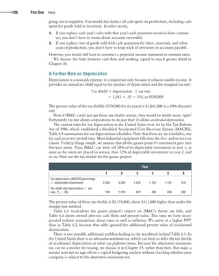
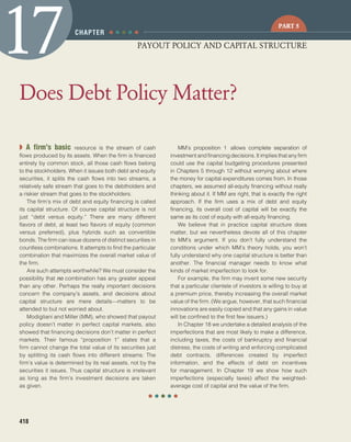
money. The payoff on the investment varies with Macbeth’s operating income, as shown
in Table 17.3. This is exactly the same set of payoffs as the investor would get by buying
one share in the levered company. [Compare the last two lines of Tables 17.2 and 17.3.]
Therefore, a share in the levered company must also sell for $10. If Macbeth goes ahead
and borrows, it will not allow investors to do anything that they could not do already, and
so it will not increase value.”
The argument that you are using is exactly the same as the one MM used to prove
proposition 1.
Consider now the implications of MM’s proposition 1 for the expected returns on Macbeth
stock:
Current Structure:
All Equity
Proposed Structure:
Equal Debt and Equity
Expected earnings per share ($) 1.50 2.00
Price per share ($) 10 10
Expected return on share (%) 15 20
Leverage increases the expected stream of earnings per share but not the share price. The
reason is that the change in the expected earnings stream is exactly offset by a change in
the rate at which the earnings are discounted. The expected return on the share (which for
a perpetuity is equal to the earnings–price ratio) increases from 15% to 20%. We now show
how this comes about.
The expected return on Macbeth’s assets rA is equal to the expected operating income
divided by the total market value of the firm’s securities:
Expected return on assets 5 rA 5
expected operating income
market value of all securities
We have seen that in perfect capital markets the company’s borrowing decision does
not affect either the firm’s operating income or the total market value of its securities.
Therefore the borrowing decision also does not affect the expected return on the firm’s
assets rA.
Suppose that an investor holds all of a company’s debt and all of its equity. This investor
is entitled to all the firm’s operating income; therefore, the expected return on the portfolio
is just rA.
17-2 Financial Risk and Expected Returns
Operating Income ($)
500 1,000 1,500 2,000
Earnings on two shares ($) 1 2 3 4
Less interest at 10% ($) 1 1 1 1
Net earnings on investment ($) 0 1 2 3
Return on $10 investment (%) 0 10 20 30
Expected
outcome
◗ TABLE 17.3
Individual investors
can replicate Macbeth’s
leverage.

confirming pages
The expected return on a portfolio is equal to a weighted average of the expected returns
on the individual holdings. Therefore the expected return on a portfolio consisting of all
the firm’s securities is
Expected return on assets 5 1proportion in debt 3 expected return on debt2
1 1proportion in equity 3 expected return on equity2
rA 5 a
D
D 1 E
3 rDb 1 a
E
D 1 E
3 rEb
This formula is of course an old friend from Chapter 9. The overall expected return rA is
called the company cost of capital or the weighted-average cost of capital (WACC).
We can turn the formula around to solve for rE, the expected return to equity for a
levered firm:
Expected return on equity 5 expected return on assets
1 1expected return on assets 2 expected return on debt2
3 debt–equity ratio
rE 5 rA 1 1rA 2 rD 2
D
E
Proposition 2
This is MM’s proposition 2: The expected rate of return on the common stock of a levered
firm increases in proportion to the debt–equity ratio (D/E), expressed in market values; the
rate of increase depends on the spread between rA, the expected rate of return on a portfolio
of all the firm’s securities, and rD, the expected return on the debt. Note that rE ϭ rA if the
firm has no debt.
We can check out this formula for Macbeth Spot Removers. Before the decision to
borrow
rE 5 rA 5
expected operating income
market value of all securities
5
1,500
10,000
5 .15, or 15%
If the firm goes ahead with its plan to borrow, the expected return on assets rA is still 15%.
The expected return on equity is
rE 5 rA 1 1rA 2 rD 2
D
E
5 .15 1 1.15 2 .102
5,000
5,000
5 .20, or 20%
When the firm was unlevered, equity investors demanded a return of rA. When the firm is
levered, they require a premium of (rA Ϫ rD)D/E to compensate for the extra risk.
MM’s proposition 1 says that financial leverage has no effect on shareholders’ wealth.
Proposition 2 says that the rate of return they can expect to receive on their shares increases
as the firm’s debt–equity ratio increases. How can shareholders be indifferent to increased
leverage when it increases expected return? The answer is that any increase in expected
return is exactly offset by an increase in risk and therefore in shareholders’ required rate of
return.
Look at what happens to the risk of Macbeth shares if it moves to equal debt–equity
proportions. Table 17.4 shows how a shortfall in operating income affects the payoff to the
shareholders.

confirming pages
The debt–equity proportion does not affect the dollar risk borne by equityholders. Sup-
pose operating income drops from $1,500 to $500. Under all-equity financing, equity earn-
ings drop by $1 per share. There are 1,000 outstanding shares, and so total equity earnings
fall by $1 ϫ 1,000 ϭ $1,000. With 50% debt, the same drop in operating income reduces
earnings per share by $2. But there are only 500 shares outstanding, and so total equity
income drops by $2 ϫ 500 ϭ $1,000, just as in the all-equity case.
However, the debt–equity choice does amplify the spread of percentage returns. If the
firm is all-equity-financed, a decline of $1,000 in the operating income reduces the return
on the shares by 10%. If the firm issues risk-free debt with a fixed interest payment of $500
a year, then a decline of $1,000 in the operating income reduces the return on the shares by
20%. In other words, the effect of the proposed leverage is to double the amplitude of the
swings in Macbeth’s shares. Whatever the beta of the firm’s shares before the refinancing,
it would be twice as high afterward.
Now you can see why investors require higher returns on levered equity. The required
return simply rises to match the increased risk.
If operating income falls from $1,500 to $500 Change
No debt: Earnings per share $1.50 $.50 Ϫ$1.00
Return 15% 5% Ϫ10%
50% debt: Earnings per share $2.00 0 Ϫ$2.00
Return 20% 0 Ϫ20%
◗ TABLE 17.4 Financial leverage increases the risk of Macbeth shares. A $1,000 drop
in operating income reduces earnings per share by $1 with all-equity financing, but by $2 with
50% debt.
EXAMPLE 17.1 ● Leverage and the Cost of Equity
Let us revisit a numerical example from Chapter 9. We looked at a company with the
following market-value balance sheet:
Asset value 100 Debt (D) 30 at rD ϭ 7.5%
Equity (E) 70 at rE ϭ 15%
Asset value 100 Firm value (V) 100
and an overall cost of capital of:
rA 5 rD
D
V
1 rE
E
V
5 a7.5 3
30
100
b 1 a15 3
70
100
b 5 12.75%
If the firm is contemplating investment in a project that has the same risk as the firm’s exist-
ing business, the opportunity cost of capital for this project is the same as the firm’s cost of
capital; in other words, it is 12.75%.
What would happen if the firm issued an additional 10 of debt and used the cash to
repurchase 10 of its equity? The revised market-value balance sheet is

confirming pages
Asset value 100 Debt (D) 40
Equity (E) 60
Asset value 100 Firm value (V) 100
The change in financial structure does not affect the amount or risk of the cash flows on
the total package of debt and equity. Therefore, if investors required a return of 12.75% on
the total package before the refinancing, they must require a 12.75% return on the firm’s
assets afterward.
Although the required return on the package of debt and equity is unaffected, the
change in financial structure does affect the required return on the individual securities.
Since the company has more debt than before, the debtholders are likely to demand a
higher interest rate. Suppose that the expected return on the debt rises to 7.875%. Now you
can write down the basic equation for the return on assets
rA 5 rD
D
V
1 rE
E
V
5 a7.875 3
40
100
b 1 arE 3
60
100
b 5 12.75%
and solve for the return on equity rE ϭ 16.0%.
Increasing the amount of debt increased debtholder risk and led to a rise in the
return that debtholders required (rdebt rose from 7.5 to 7.875%). The higher leverage
also made the equity riskier and increased the return that shareholders required (rE
rose from 15% to 16%). The weighted-average return on debt and equity remained at
12.75%:
rA 5 1rD 3 .42 1 1rE 3 .62
5 17.875 3 .42 1 116 3 62 5 12.75%
Suppose that the company decided instead to repay all its debt and to replace it with equity.
In that case all the cash flows would go to the equityholders. The company cost of capital,
rA, would stay at 12.75%, and rE would also be 12.75%.
How Changing Capital Structure Affects Beta
We have looked at how changes in financial structure affect expected return. Let us now
look at the effect on beta.
The stockholders and debtholders both receive a share of the firm’s cash flows, and both
bear part of the risk. For example, if the firm’s assets turn out to be worthless, there will be
no cash to pay stockholders or debtholders. But debtholders usually bear much less risk
than stockholders. Debt betas of large firms are typically in the range of .1 to .3.
If you owned a portfolio of all the firm’s securities, you wouldn’t share the cash flows
with anyone. You wouldn’t share the risks with anyone either; you would bear them all.
Thus the firm’s asset beta is equal to the beta of a portfolio of all the firm’s debt and its
equity.
The beta of this hypothetical portfolio is just a weighted average of the debt and equity
betas:
␤A 5 ␤portfolio 5 ␤D
D
V
1 ␤E
E
V
● ● ● ● ●

confirming pages
Think back to our example. If the debt before the refinancing has a beta of .1 and the equity
has a beta of 1.1, then
␤A 5 a.1 3
30
100
b 1 a1.1 3
70
100
b 5 .8
What happens after the refinancing? The risk of the total package is unaffected, but both
the debt and the equity are now more risky. Suppose that the debt beta increases to .2. We
can work out the new equity beta:
␤A 5 ␤portfolio 5 ␤D
D
V
1 ␤E
E
V
.8 5 a.2 3
40
100
b 1 a␤E 3
60
100
b
␤E 5 1.2
Our example shows how borrowing creates financial leverage or gearing. Financial leverage
does not affect the risk or the expected return on the firm’s assets, but it does push up the
risk of the common stock. Shareholders demand a correspondingly higher return because
of this financial risk.
Now you can see how to unlever betas, that is, how to go from an observed ␤E to ␤A. You
have the equity beta, say, 1.2. You also need the debt beta, say, .2, and the relative market
values of debt (D/V) and equity (E/V). If debt accounts for 40% of overall value V, then
the unlevered beta is
␤A 5 a.2 3
40
100
b 1 a1.2 3
60
100
b 5 .8
This runs the previous example in reverse. Just remember the basic relationship:
␤A 5 ␤portfolio 5 ␤Da
D
V
b 1 ␤Ea
E
V
b
MM’s propositions warn us that higher leverage increases both expected equity returns
and equity risk. It does not increase shareholder value. Having worked through the example
of Macbeth, this much should now seem obvious. But watch out for hidden changes in
leverage, such as a decision to lease new equipment or to underfund the pension scheme.
Do not interpret any resultant increase in the expected equity return as creating additional
shareholder value.
What did financial experts think about debt policy before MM? It is not easy to say because
with hindsight we see that they did not think too clearly.4
However, a “traditional” position
emerged in response to MM. To understand it, we have to return to the weighted-average
cost of capital.
Figure 17.2 sums up the implications of MM’s propositions for the costs of debt and
equity and the weighted-average cost of capital. The figure assumes that the firm’s bonds
are essentially risk-free at low debt levels. Thus rD is independent of D/E, and rE increases
linearly as D/E increases. As the firm borrows more, the risk of default increases and the
firm is required to pay higher rates of interest. Proposition 2 predicts that when this occurs
4
Financial economists in 20 years may remark on Brealey, Myers, and Allen’s blind spots and clumsy reasoning. On the other
hand, they may not remember us at all.
17-3 The Weighted-Average Cost of Capital

confirming pages
the rate of increase in rE slows down. This is also shown in Figure 17.2. The more debt the
firm has, the less sensitive rE is to further borrowing.
Why does the slope of the rE line in Figure 17.2 taper off as D/E increases? Essentially
because holders of risky debt bear some of the firm’s business risk. As the firm borrows
more, more of that risk is transferred from stockholders to bondholders.
Two Warnings
Sometimes the objective in financing decisions is stated not as “maximize overall market
value” but as “minimize the weighted-average cost of capital.” If MM’s proposition 1 holds,
then these are equivalent objectives. If MM’s proposition 1 does not hold, then the capital
structure that maximizes the value of the firm also minimizes the weighted-average cost of
capital, provided that operating income is independent of capital structure. Remember that
the weighted-average cost of capital is the expected rate of return on the market value of all
of the firm’s securities. Anything that increases the value of the firm reduces the weighted-
average cost of capital if operating income is constant. But if operating income is varying
too, all bets are off.
In Chapter 18 we show that financial leverage can affect operating income in several
ways. Therefore maximizing the value of the firm is not always equivalent to minimizing
the weighted-average cost of capital.
Warning 1 Shareholders want management to increase the firm’s value. They are more
interested in being rich than in owning a firm with a low weighted-average cost of capital.
Warning 2 Trying to minimize the weighted-average cost of capital seems to encour-
age logical short circuits like the following. Suppose that someone says, “Shareholders
demand—and deserve—higher expected rates of return than bondholders do. Therefore
debt is the cheaper capital source. We can reduce the weighted-average cost of capital
by borrowing more.” But this doesn’t follow if the extra borrowing leads stockholders to
demand a still higher expected rate of return. According to MM’s proposition 2 the cost
of equity capital rE increases by just enough to keep the weighted-average cost of capital
constant.
Risk-free debt Risky debt debt
equity
D
E
Rates of return
rE = Expected return on equity
rA = Expected return on assets
rD = Expected return on debt
=
◗ FIGURE 17.2
MM’s proposition 2.
The expected return
on equity rE increases
linearly with the debt–
equity ratio so long as
debt is risk-free. But
if leverage increases
the risk of the debt,
debtholders demand
a higher return on the
debt. This causes the
rate of increase in rE to
slow down.

confirming pages
This is not the only logical short circuit you are likely to encounter. We have cited two
more in Problem 15 at the end of this chapter.
Rates of Return on Levered Equity—The Traditional Position
You may ask why we have even mentioned the aim of minimizing the weighted-average
cost of capital if it is often wrong or confusing. We had to because the traditionalists accept
this objective and argue their case in terms of it.
The logical short circuit we just described rested on the assumption that rE, the expected
rate of return demanded by stockholders, does not rise, or rises very slowly, as the firm bor-
rows more. Suppose, just for the sake of argument, that this is true. Then rA, the weighted-
average cost of capital, must decline as the debt–equity ratio rises.
The traditionalists’ position is shown in Figure 17.3. They say that a moderate degree of
financial leverage may increase the expected equity return rE, but not as much as predicted
by MM’s proposition 2. But irresponsible firms that borrow excessively find rE shooting up
faster than MM predict. Therefore the weighted-average cost of capital declines at first, then
rises. It reaches a minimum at some intermediate debt ratio. Remember that minimizing
the weighted-average cost of capital is equivalent to maximizing firm value if operating
income is not affected by borrowing.
Two arguments could be advanced in support of this position. First, perhaps investors
do not notice or appreciate the financial risk created by moderate borrowing, although they
wake up when debt is “excessive.” If so, stockholders in moderately leveraged firms may
accept a lower rate of return than they really should.
That seems naive.5
The second argument is better. It accepts MM’s reasoning as
applied to perfect capital markets but holds that actual markets are imperfect. Because
5
This first argument may reflect a confusion between financial risk and the risk of default. Default is not a serious threat when
borrowing is moderate; stockholders worry about it only when the firm goes “too far.” But stockholders bear financial risk—in the
form of increased volatility of rates of return and a higher beta—even when the chance of default is nil.
Rates of return
debt
equity
D
E
=
rE (MM)
rE (traditional)
rA (traditional)
rA (MM)
rD
Traditionalists believe there is an optimal
debt–equity ratio that minimizes rA.
◗ FIGURE 17.3
The dashed lines
show MM’s view of
the effect of lever-
age on the expected
return on equity rE and
the weighted-average
cost of capital rA. (See
Figure 17.2.) The solid
lines show the traditional
view. Traditionalists say
that borrowing at first
increases rE more slowly
than MM predict but that
rE shoots up with exces-
sive borrowing. If so, the
weighted-average cost of
capital can be minimized
if you use just the right
amount of debt.

confirming pages
of these imperfections, firms that borrow may provide a valuable service for investors.
If so, levered shares might trade at premium prices compared to their theoretical values
in perfect markets.
Suppose that corporations can borrow more cheaply than individuals. Then it would
pay investors who want to borrow to do so indirectly by holding the stock of levered firms.
They would be willing to live with expected rates of return that do not fully compensate
them for the business and financial risk they bear.
Is corporate borrowing really cheaper? It’s hard to say. Interest rates on home mortgages
are not too different from rates on high-grade corporate bonds.6
Rates on margin debt
(borrowing from a stockbroker with the investor’s shares tendered as security) are not too
different from the rates firms pay banks for short-term loans.
There are some individuals who face relatively high interest rates, largely because of the
costs lenders incur in making and servicing small loans. There are economies of scale in
borrowing. A group of small investors could do better by borrowing via a corporation, in
effect pooling their loans and saving transaction costs.7
Suppose that this class of investors is large, both in number and in the aggregate wealth
it brings to capital markets. That creates a clientele for whom corporate borrowing is better
than personal borrowing. That clientele would, in principle, be willing to pay a premium
for the shares of a levered firm.
But maybe it doesn’t have to pay a premium. Perhaps smart financial managers long ago
recognized this clientele and shifted the capital structures of their firms to meet its needs.
The shifts would not have been difficult or costly. But if the clientele is now satisfied, it no
longer needs to pay a premium for levered shares. Only the financial managers who first
recognized the clientele extracted any advantage from it.
Maybe the market for corporate leverage is like the market for automobiles. Americans
need millions of automobiles and are willing to pay thousands of dollars apiece for them.
But that doesn’t mean that you could strike it rich by going into the automobile business.
You’re at least 80 years too late.
Today’s Unsatisfied Clienteles Are Probably
Interested in Exotic Securities
So far we have made little progress in identifying cases where firm value might plausibly
depend on financing. But our examples illustrate what smart financial managers look for.
They look for an unsatisfied clientele, investors who want a particular kind of financial
instrument but because of market imperfections can’t get it or can’t get it cheaply.
MM’s proposition 1 is violated when the firm, by imaginative design of its capital struc-
ture, can offer some financial service that meets the needs of such a clientele. Either the
service must be new and unique or the firm must find a way to provide some old service
more cheaply than other firms or financial intermediaries can.
Now, is there an unsatisfied clientele for garden-variety debt or levered equity? We
doubt it. But perhaps you can invent an exotic security and uncover a latent demand
for it.
In the next several chapters we will encounter a number of new securities that have been
invented by companies and advisers. These securities take the company’s basic cash flows
6
One of the authors once obtained a home mortgage at a rate 1/2 percentage point less than the contemporaneous yield on long-
term AAA bonds.
7
Even here there are alternatives to borrowing on personal account. Investors can draw down their savings accounts or sell a por-
tion of their investment in bonds. The impact of reductions in lending on the investor’s balance sheet and risk position is exactly
the same as increases in borrowing.

confirming pages
and repackage them in ways that are thought to be more attractive to investors. However,
while inventing these new securities is easy, it is more difficult to find investors who will
rush to buy them.
Imperfections and Opportunities
The most serious capital market imperfections are often those created by government. An
imperfection that supports a violation of MM’s proposition 1 also creates a money-making
opportunity. Firms and intermediaries will find some way to reach the clientele of investors
frustrated by the imperfection.
For many years the U.S. government imposed a limit on the rate of interest that
could be paid on savings accounts. It did so to protect savings institutions by limiting
competition for their depositors’ money. The fear was that depositors would run off in
search of higher yields, causing a cash drain that savings institutions would not be able
to meet.
These regulations created an opportunity for firms and financial institutions to design
new savings schemes that were not subject to the interest-rate ceilings. One invention was
the floating-rate note, first issued in 1974 by Citicorp, and with terms designed to appeal to
individual investors. Floating-rate notes are medium-term debt securities whose interest
payments “float” with short-term interest rates. On the Citicorp issue, for example, the cou-
pon rate used to calculate each semiannual interest payment was set at 1 percentage point
above the contemporaneous yield on Treasury bills. The holder of the Citicorp note was
therefore protected against fluctuating interest rates, because Citicorp sent a larger check
when interest rates rose (and, of course, a smaller check when rates fell).
Citicorp evidently found an untapped clientele of investors, for it was able to raise
$650 million in the first offering. The success of the issue suggests that Citicorp was able
to add value by changing its capital structure. However, other companies were quick to
jump on Citicorp’s bandwagon, and within five months an additional $650 million of
floating-rate notes were issued by other companies. By the mid-1980s about $43 billion
of floating-rate securities were outstanding, and now floating-rate debt securities seem
ubiquitous.
Interest-rate regulation also provided financial institutions with an opportunity to create
value by offering money-market funds. These are mutual funds invested in Treasury bills,
commercial paper, and other high-grade, short-term debt instruments. Any saver with a few
thousand dollars to invest can gain access to these instruments through a money-market fund
and can withdraw money at any time by writing a check against his or her fund balance. Thus
the fund resembles a checking or savings account that pays close to market interest rates.
These money-market funds have become enormously popular. By 2009 their assets had risen
to $3.7 trillion.8
Long before interest-rate ceilings were finally removed, most of the gains had gone out
of issuing the new securities to individual investors. Once the clientele was finally satisfied,
MM’s proposition 1 was restored (until the government creates a new imperfection). The
moral of the story is this: If you ever find an unsatisfied clientele, do something right away,
or capital markets will evolve and steal it from you.
This is actually an encouraging message for the economy as a whole. If MM are right,
investors’ demands for different types of securities are satisfied at minimal cost. The cost
8
Money-market funds are not totally safe. In 2008 the Reserve Primary Fund incurred heavy losses on its holdings of Lehman
Brothers debt and became only the second money-market fund in history to “break the buck” by paying investors 97 cents in the
dollar.

confirming pages
of capital will reflect only business risk. Capital will flow to companies with positive-
NPV investments, regardless of the companies’ capital structures. This is the efficient
outcome.
MM left us a simple message. When the firm changes its mix of debt and equity securities,
the risk and expected returns of these securities change, but the company’s overall cost of
capital does not change.
Now if you think that message is too neat and simple, you’re right. The complications
are spelled out in the next two chapters. But we must note one complication here: Interest
paid on a firm’s borrowing can be deducted from taxable income. Thus the after-tax cost
of debt is rD(1 Ϫ Tc), where Tc is the marginal corporate tax rate. So, when companies dis-
count an average-risk project, they do not use the company cost of capital as we have just
computed it. Instead they use the after-tax cost of debt to compute the after-tax weighted-
average cost of capital or WACC:
After-tax WACC 5 rD 11 2 Tc 2
D
V
1 rE
E
V
We briefly introduced this formula in Chapter 9, where we used it to estimate the weighted-
average cost of capital for Union Pacific. In 2009 Union Pacific’s long-term borrowing rate
was rD ϭ 7.8%, and its estimated cost of equity was rE ϭ 9.9%. With a 35% corporate tax
rate, the after-tax cost of debt was rD(1 Ϫ Tc) ϭ 7.8(1 Ϫ .35) ϭ 5.1%. The ratio of debt to
overall company value was D/V ϭ 31.5%. Therefore
After-tax WACC 5 rD 11 2 Tc 2
D
V
1 rE
E
V
5 11 2 .352 3 7.8 3 .315 1 9.9 3 .685 5 8.4%
MM’s proposition 2 states that in the absence of taxes the company cost of capital stays the
same regardless of the amount of leverage. But, if companies receive a tax shield on their
interest payments, then the after-tax WACC declines as debt increases. This is illustrated
in Figure 17.4, which shows how Union Pacific’s WACC changes as the debt–equity ratio
changes.
17-4 A Final Word on the After-Tax Weighted-Average Cost of Capital
Debt–equity ratio (D/E)
Return,%
.00 .70.60.55 .65.50.10 .15.05 .20 .25 .30 .35 .45.40
6
7
8
9
10
11
Opportunity cost of capital (r)
Cost of debt (rD)
Cost of equity (rE)
WACC
◗ FIGURE 17.4
Estimated after-tax
WACC for Union Pacific
at different debt–
equity ratios. The figure
assumes rE ϭ 9.9%
at a 31.5% debt ratio
(equivalent to a 46%
debt–equity ratio) and
a borrowing rate of
rD ϭ 7.8%. Notice that
the debt interest rate is
assumed to increase with
the debt–equity ratio.

confirming pages
Think of the financial manager as taking all of the firm’s real assets and selling them to investors
as a package of securities. Some financial managers choose the simplest package possible: all-
equity financing. Some end up issuing dozens of debt and equity securities. The problem is to
find the particular combination that maximizes the market value of the firm.
Modigliani and Miller’s (MM’s) famous proposition 1 states that no combination is better
than any other—that the firm’s overall market value (the value of all its securities) is independent
of capital structure. Firms that borrow do offer investors a more complex menu of securities, but
investors yawn in response. The menu is redundant. Any shift in capital structure can be dupli-
cated or “undone” by investors. Why should they pay extra for borrowing indirectly (by holding
shares in a levered firm) when they can borrow just as easily and cheaply on their own accounts?
MM agree that borrowing raises the expected rate of return on shareholders’ investments. But
it also increases the risk of the firm’s shares. MM show that the higher risk exactly offsets the
increase in expected return, leaving stockholders no better or worse off.
Proposition 1 is an extremely general result. It applies not just to the debt–equity trade-
off but to any choice of financing instruments. For example, MM would say that the choice
between long-term and short-term debt has no effect on firm value.
The formal proofs of proposition 1 all depend on the assumption of perfect capital markets.
MM’s opponents, the “traditionalists,” argue that market imperfections make personal borrow-
ing excessively costly, risky, and inconvenient for some investors. This creates a natural clientele
willing to pay a premium for shares of levered firms. The traditionalists say that firms should
borrow to realize the premium.
But this argument is incomplete. There may be a clientele for levered equity, but that is not
enough; the clientele has to be unsatisfied. There are already thousands of levered firms avail-
able for investment. Is there still an unsatiated clientele for garden-variety debt and equity? We
doubt it.
Proposition 1 is violated when financial managers find an untapped demand and satisfy it by
issuing something new and different. The argument between MM and the traditionalists finally
boils down to whether this is difficult or easy. We lean toward MM’s view: Finding unsatisfied
clienteles and designing exotic securities to meet their needs is a game that’s fun to play but
hard to win.
If MM are right, the overall cost of capital—the expected rate of return on a portfolio of all
the firm’s outstanding securities—is the same regardless of the mix of securities issued to finance
the firm. The overall cost of capital is usually called the company cost of capital or the weighted-
average cost of capital (WACC). MM say that WACC doesn’t depend on capital structure. But
MM assume away lots of complications. The first complication is taxes. When we recognize
that debt interest is tax-deductible, and compute WACC with the after-tax interest rate, WACC
declines as the debt ratio increases. There is more—lots more—on taxes and other complications
in the next two chapters.
SUMMARY
● ● ● ● ●
● ● ● ● ●
The fall 1988 issue of the Journal of Economic Perspectives contains a collection of articles, including
one by Modigliani and Miller, which review and assess the MM propositions. The summer 1989 issue of
Financial Management contains three more articles under the heading “Reflections on the MM Proposi-
tions 30 Years Later.”
Two surveys of financial innovation include:
K. A. Karow, G. R. Erwin, and J. J. McConnell, “Survey of U.S. Corporate Financing Innova-
tions: 1970–1997,” Journal of Applied Corporate Finance 12 (Spring 1999), pp. 55–69.
P. Tufano, “Financial Innovation,” in G. M. Constantinides, M. Harris, and R. Stulz (eds.),
Handbook of the Economics of Finance, Vol 1A (Amsterdam: Elsevier/North-Holland, 2003).
FURTHER
READING

confirming pages
BASIC
1. Ms. Kraft owns 50,000 shares of the common stock of Copperhead Corporation with a
market value of $2 per share, or $100,000 overall. The company is currently financed as
follows:
Book Value
Common stock (8 million shares) $2 million
Short-term loans $2 million
Copperhead now announces that it is replacing $1 million of short-term debt with an
issue of common stock. What action can Ms. Kraft take to ensure that she is entitled to
exactly the same proportion of profits as before?
2. Spam Corp. is financed entirely by common stock and has a beta of 1.0. The firm is
expected to generate a level, perpetual stream of earnings and dividends. The stock has
a price–earnings ratio of 8 and a cost of equity of 12.5%. The company’s stock is selling
for $50. Now the firm decides to repurchase half of its shares and substitute an equal
value of debt. The debt is risk-free, with a 5% interest rate. The company is exempt from
corporate income taxes. Assuming MM are correct, calculate the following items after the
refinancing:
a. The cost of equity.
b. The overall cost of capital (WACC).
c. The price–earnings ratio.
d. The stock price.
e. The stock’s beta.
3. The common stock and debt of Northern Sludge are valued at $50 million and $30 million,
respectively. Investors currently require a 16% return on the common stock and an 8%
return on the debt. If Northern Sludge issues an additional $10 million of common stock
and uses this money to retire debt, what happens to the expected return on the stock?
Assume that the change in capital structure does not affect the risk of the debt and that
there are no taxes.
4. Suppose that Macbeth Spot Removers issues only $2,500 of debt and uses the proceeds to
repurchase 250 shares.
a. Rework Table 17.2 to show how earnings per share and share return now vary with
operating income.
b. If the beta of Macbeth’s assets is .8 and its debt is risk-free, what would be the beta of
the equity after the debt issue?
PROBLEM SETS
Miller reviews the MM propositions in:
M. H. Miller, “The Modigliani-Miller Propositions after Thirty Years,” Journal of Applied
Corporate Finance 2 (Spring 1989), pp. 6–18.
For a skeptic’s view of MM’s arguments see:
S. Titman, “The Modigliani-Miller Theorem and the Integration of Financial Markets,”
Financial Management 31 (Spring 2002), pp. 101–115.
● ● ● ● ●

confirming pages
5. True or false?
a. MM’s propositions assume perfect financial markets, with no distorting taxes or other
imperfections.
b. MM’s proposition 1 says that corporate borrowing increases earnings per share but
reduces the price–earnings ratio.
c. MM’s proposition 2 says that the cost of equity increases with borrowing and that the
increase is proportional to D/V, the ratio of debt to firm value.
d. MM’s proposition 2 assumes that increased borrowing does not affect the interest rate
on the firm’s debt.
e. Borrowing does not increase financial risk and the cost of equity if there is no risk of
bankruptcy.
f. Borrowing increases firm value if there is a clientele of investors with a reason to prefer debt.
6. Look back to Section 17.1. Suppose that Ms. Macbeth’s investment bankers have informed
her that since the new issue of debt is risky, debtholders will demand a return of 12.5%,
which is 2.5% above the risk-free interest rate.
a. What are rA and rE?
b. Suppose that the beta of the unlevered stock was .6. What will ␤A, ␤E, and ␤D be after
the change to the capital structure?
7. Note the two blank graphs in Figure 17.5 below. On graph (a), assume MM are right,
and plot the relationship between financial leverage (debt-equity ratio) and (i) the rates of
return on debt and equity and (ii) the weighted-average cost of capital. Then fill in graph
(b), assuming the traditionalists are right.
8. Gaucho Services starts life with all-equity financing and a cost of equity of 14%. Suppose
it refinances to the following market-value capital structure:
Debt (D) 45% at rD ϭ 9.5%
Equity (E) 55%
Use MM’s proposition 2 to calculate the new cost of equity. Gaucho pays taxes at a mar-
ginal rate of Tc ϭ 40%. Calculate Gaucho’s after-tax weighted-average cost of capital.
INTERMEDIATE
9. Companies A and B differ only in their capital structure. A is financed 30% debt and 70%
equity; B is financed 10% debt and 90% equity. The debt of both companies is risk-free.
a. Rosencrantz owns 1% of the common stock of A. What other investment package
would produce identical cash flows for Rosencrantz?
b. Guildenstern owns 2% of the common stock of B. What other investment package
would produce identical cash flows for Guildenstern?
Rates of return
Leverage
(a)
Rates of return
Leverage
(b)
◗ FIGURE 17.5
See Problem 7.

confirming pages
c. Show that neither Rosencrantz nor Guildenstern would invest in the common stock of
B if the total value of company A were less than that of B.
10. Here is a limerick:
There once was a man named Carruthers,
Who kept cows with miraculous udders.
He said, “Isn’t this neat?
They give cream from one teat,
And skim milk from each of the others!”
What is the analogy between Mr. Carruthers’s cows and firms’ financing decisions? What
would MM’s proposition 1, suitably adapted, say about the value of Mr. Carruthers’s cows?
Explain.
11. Executive Chalk is financed solely by common stock and has outstanding 25 million shares
with a market price of $10 a share. It now announces that it intends to issue $160 million
of debt and to use the proceeds to buy back common stock.
a. How is the market price of the stock affected by the announcement?
b. How many shares can the company buy back with the $160 million of new debt that it
issues?
c. What is the market value of the firm (equity plus debt) after the change in capital
structure?
d. What is the debt ratio after the change in structure?
e. Who (if anyone) gains or loses?
Now try the next question.
12. Executive Cheese has issued debt with a market value of $100 million and has outstand-
ing 15 million shares with a market price of $10 a share. It now announces that it intends
to issue a further $60 million of debt and to use the proceeds to buy back common
stock. Debtholders, seeing the extra risk, mark the value of the existing debt down to
$70 million.
a. How is the market price of the stock affected by the announcement?
b. How many shares can the company buy back with the $60 million of new debt that it
issues?
c. What is the market value of the firm (equity plus debt) after the change in capital
structure?
d. What is the debt ratio after the change in structure?
e. Who (if anyone) gains or loses?
13. Hubbard’s Pet Foods is financed 80% by common stock and 20% by bonds. The expected
return on the common stock is 12% and the rate of interest on the bonds is 6%. Assum-
ing that the bonds are default-risk free, draw a graph that shows the expected return of
Hubbard’s common stock (rE) and the expected return on the package of common stock
and bonds (rA) for different debt–equity ratios.
14. “MM totally ignore the fact that as you borrow more, you have to pay higher rates of inter-
est.” Explain carefully whether this is a valid objection.
15. Indicate what’s wrong with the following arguments:
a. “As the firm borrows more and debt becomes risky, both stockholders and bondholders
demand higher rates of return. Thus by reducing the debt ratio we can reduce both the
cost of debt and the cost of equity, making everybody better off.”
b. “Moderate borrowing doesn’t significantly affect the probability of financial distress
or bankruptcy. Consequently moderate borrowing won’t increase the expected rate of
return demanded by stockholders.”

confirming pages
16. Each of the following statements is false or at least misleading. Explain why in each case.
a. “A capital investment opportunity offering a 10% DCF rate of return is an attractive
project if it can be 100% debt-financed at an 8% interest rate.”
b. “The more debt the firm issues, the higher the interest rate it must pay. That is one
important reason why firms should operate at conservative debt levels.”
17. Can you invent any new kinds of debt that might be attractive to investors? Why do you
think they have not been issued?
18. Imagine a firm that is expected to produce a level stream of operating profits. As leverage
is increased, what happens to:
a. The ratio of the market value of the equity to income after interest?
b. The ratio of the market value of the firm to income before interest if (i) MM are right
and (ii) the traditionalists are right?
19. Archimedes Levers is financed by a mixture of debt and equity. You have the following
information about its cost of capital:
rE ϭ rD ϭ 12% rA ϭ
␤E ϭ 1.5 ␤D ϭ ␤A ϭ
rf ϭ 10% rm ϭ 18% D/V ϭ .5
Can you fill in the blanks?
20. Look back to Problem 19. Suppose now that Archimedes repurchases debt and issues
equity so that D/V ϭ .3. The reduced borrowing causes rD to fall to 11%. How do the
other variables change?
21. Omega Corporation has 10 million shares outstanding, now trading at $55 per share.
The firm has estimated the expected rate of return to shareholders at about 12%. It
has also issued long-term bonds at an interest rate of 7%. It pays tax at a marginal rate
of 35%.
a. What is Omega’s after-tax WACC?
b. How much higher would WACC be if Omega used no debt at all? (Hint: For this
problem you can assume that the firm’s overall beta [␤A] is not affected by its capital
structure or the taxes saved because debt interest is tax-deductible.)
22. Gamma Airlines has an asset beta of 1.5. The risk-free interest rate is 6%, and the market
risk premium is 8%. Assume the capital asset pricing model is correct. Gamma pays taxes
at a marginal rate of 35%. Draw a graph plotting Gamma’s cost of equity and after-tax
WACC as a function of its debt-to-equity ratio D/E, from no debt to D/E ϭ 1.0. Assume
that Gamma’s debt is risk-free up to D/E ϭ .25. Then the interest rate increases to 6.5% at
D/E ϭ .5, 7% at D/E ϭ .8, and 8% at D/E ϭ 1.0. As in Problem 21, you can assume that
the firm’s overall beta (␤A) is not affected by its capital structure or the taxes saved because
debt interest is tax-deductible.
CHALLENGE
23. Consider the following three tickets: ticket A pays $10 if _______ is elected as president,
ticket B pays $10 if _______ is elected, and ticket C pays $10 if neither is elected. (Fill in the
blanks yourself.) Could the three tickets sell for less than the present value of $10? Could
they sell for more? Try auctioning off the tickets. What are the implications for MM’s
proposition 1?
24. People often convey the idea behind MM’s proposition 1 by various supermarket analo-
gies, for example, “The value of a pie should not depend on how it is sliced,” or, “The cost
of a whole chicken should equal the cost of assembling one by buying two drumsticks, two
wings, two breasts, and so on.”

confirming pages
Actually proposition 1 doesn’t work in the supermarket. You’ll pay less for an uncut
whole pie than for a pie assembled from pieces purchased separately. Supermarkets
charge more for chickens after they are cut up. Why? What costs or imperfections
cause proposition 1 to fail in the supermarket? Are these costs or imperfections likely
to be important for corporations issuing securities on the U.S. or world capital markets?
Explain.
25. Suppose that new security designs could be patented.9
The patent holder could restrict
use of the new design or charge other firms royalties for using it. What effect would such
patents have on MM’s capital-structure irrelevance theory?
9
So far security designs cannot be patented, but other financial applications have received patent protection. See J. Lerner, “Where
Does State Street Lead? A First Look at Finance Patents,” Journal of Finance 57 (April 2002), pp. 901–930.

● ● ● ● ●
confirming pages
440
◗ In Chapter 17 we found that debt policy rarely
matters in well-functioning capital markets with no
frictions or imperfections. Few financial managers would
accept that conclusion as a practical guideline. If debt
policy doesn’t matter, then they shouldn’t worry about
it—financing decisions could be routine or erratic—it
wouldn’t matter. Yet financial managers do worry about
debt policy. This chapter explains why.
If debt policy were completely irrelevant, then actual
debt ratios should vary randomly from firm to firm and
industry to industry. Yet almost all airlines, utilities,
banks, and real estate development companies
rely heavily on debt. And so do many firms in capital-
intensive industries such as steel, aluminum, chemicals,
petroleum, and mining. On the other hand, it is rare to
find a pharmaceutical company or advertising agency
that is not predominantly equity-financed. Glamorous
growth companies rarely use much debt despite rapid
expansion and often heavy requirements for capital.
The explanation of these patterns lies partly in the
things we left out of the last chapter. We mostly ignored
taxes. We assumed bankruptcy was cheap, quick, and
painless. It isn’t, and there are costs associated with
financial distress even if legal bankruptcy is ultimately
avoided. We ignored potential conflicts of interest
between the firm’s security holders. For example,
we did not consider what happens to the firm’s “old”
creditors when new debt is issued or when a shift
in investment strategy takes the firm into a riskier
business. We ignored the information problems that
favor debt over equity when cash must be raised from
new security issues. We ignored the incentive effects
of financial leverage on management’s investment and
payout decisions.
Now we will put all these things back in: taxes first,
then the costs of bankruptcy and financial distress. This
will lead us to conflicts of interest and to information and
incentive problems. In the end we will have to admit that
debt policy does matter.
However, we will not throw away the MM theory we
developed so carefully in Chapter 17. We’re shooting
for a theory combining MM’s insights plus the effects of
taxes, costs of bankruptcy and financial distress, and
various other complications. We’re not dropping back
to a theory based on inefficiencies in the capital market.
Instead, we want to see how well-functioning capital
markets respond to taxes and the other things covered
in this chapter.
How Much Should a
Corporation Borrow?
18 CHAPTER
PART 5
Debt financing has one important advantage under the corporate income tax system in
the U.S. and many other countries. The interest that the company pays is a tax-deductible
expense. Thus the return to bondholders escapes taxation at the corporate level.
Table 18.1 shows simple income statements for firm U, which has no debt, and firm
L, which has borrowed $1,000 at 8%. L’s tax bill is $28 less than U’s. This is the tax shield
18-1 Corporate Taxes
● ● ● ● ●

confirming pages
Chapter 18 How Much Should a Corporation Borrow? 441
provided by the debt of L. In effect the government pays 35% of the interest expense of L.
The total income that L can pay out to its bondholders and stockholders increases by that
amount.
Tax shields can be valuable assets. Suppose that the debt of L is fixed and permanent.
(That is, the company commits to refinance its present debt obligations when they mature
and to keep rolling over its debt obligations indefinitely.) Then L can look forward to a
permanent stream of cash flows of $28 per year. The risk of these flows is likely to be less
than the risk of the operating assets of L. The tax shields depend only on the corporate tax
rate1
and on the ability of L to earn enough to cover interest payments. The corporate tax
rate has been pretty stable. And the ability of L to earn its interest payments must be reason-
ably sure; otherwise it could not have borrowed at 8%. Therefore we should discount the
interest tax shields at a relatively low rate.
But what rate? One common assumption is that the risk of the tax shields is the same as
that of the interest payments generating them. Thus we discount at 8%, the expected rate
of return demanded by investors who are holding the firm’s debt:
PV1tax shield2 5
28
.08
5 $350
In effect the government assumes 35% of the $1,000 debt obligation of L.
Under these assumptions, the present value of the tax shield is independent of the return
on the debt rD. It equals the corporate tax rate Tc times the amount borrowed D:
Interest payment 5 return on debt 3 amount borrowed
5 rD 3 D
PV1tax shield2 5
corporate tax rate 3 interest payment
expected return on debt
5
TcrDD
rD
5 Tc D
1
Always use the marginal corporate tax rate, not the average rate. Average rates are often much lower than marginal rates because
of accelerated depreciation and other tax adjustments. For large corporations, the marginal rate is usually taken as the statutory
rate, which was 35% when this chapter was written (2009). However, effective marginal rates can be less than the statutory rate,
especially for smaller, riskier companies that cannot be sure that they will earn taxable income in the future.
◗ TABLE 18.1 The tax deductibility of interest increases the total income that can be paid out to
bondholders and stockholders.
Income Statement of Firm U Income Statement of Firm L
Earnings before interest and taxes $1,000 $1,000
Interest paid to bondholders 0 80
Pretax income 1,000 920
Tax at 35% 350 322
Net income to stockholders $ 650 $ 598
Total income to both bondholders
and stockholders
$0 ϩ 650 ϭ $650 $80 ϩ 598 ϭ $678
Interest tax shield (.35 ϫ interest) $0 $28

confirming pages
Of course, PV(tax shield) is less if the firm does not plan to borrow a permanent fixed
amount,2
or if it may not have enough taxable income to use the interest tax shields.3
How Do Interest Tax Shields Contribute
to the Value of Stockholders’ Equity?
MM’s proposition 1 amounts to saying that the value of a pie does not depend on how it is
sliced. The pie is the firm’s assets, and the slices are the debt and equity claims. If we hold
the pie constant, then a dollar more of debt means a dollar less of equity value.
But there is really a third slice, the government’s. Look at Table 18.2. It shows an
expanded balance sheet with pretax asset value on the left and the value of the government’s
tax claim recognized as a liability on the right. MM would still say that the value of the
pie—in this case pretax asset value—is not changed by slicing. But anything the firm can do
to reduce the size of the government’s slice obviously makes stockholders better off. One
thing it can do is borrow money, which reduces its tax bill and, as we saw in Table 18.1,
increases the cash flows to debt and equity investors. The after-tax value of the firm (the
sum of its debt and equity values as shown in a normal market value balance sheet) goes
up by PV(tax shield).
Recasting Merck’s Capital Structure
Merck is a large, successful firm that uses relatively little long-term debt. Table 18.3(a)
shows simplified book and market value balance sheets for Merck in December 2008.
Suppose that you were Merck’s financial manager with complete responsibility for its
capital structure. You decide to borrow an additional $1 billion on a permanent basis and
use the proceeds to repurchase shares.
Table 18.3(b) shows the new balance sheets. The book version simply has $1,000 million
more long-term debt and $1,000 million less equity. But we know that Merck’s assets must
be worth more because its tax bill has been reduced by 35% of the interest on the new
2
In this example, we assume that the amount of debt is fixed and stable over time. The natural alternative assumption is a fixed
ratio of debt to firm value. If the ratio is fixed, then the level of debt and the amount of interest tax shields will fluctuate as firm
value fluctuates. In that case projected interest tax shields can’t be discounted at the cost of debt. We cover this point in detail in
the next chapter.
3
If the income of L does not cover interest in some future year, the tax shield is not necessarily lost. L can carry back the loss and
receive a tax refund up to the amount of taxes paid in the previous two years. If L has a string of losses, and thus no prior tax pay-
ments that can be refunded, then losses can be carried forward and used to shield income in later years.
Normal Balance Sheet (Market Values)
Asset value of (present value
of after-tax cash flows)
Total assets
Debt
Equity
Total value
Expanded Balance Sheet (Market Values)
Pretax asset value (present value
of pretax cash flows)
Debt
Government’s claim (present
value of future taxes)
Total pretax assets
Equity
Total pretax value
◗ TABLE 18.2
Normal and expanded
market value balance
sheets. In a normal
balance sheet, assets are
valued after tax. In the
expanded balance sheet,
assets are valued pretax,
and the value of the
government’s tax claim
is recognized on the
right-hand side. Interest
tax shields are valuable
because they reduce the
government’s claim.

confirming pages
debt. In other words, Merck has an increase in PV(interest tax shield), which is worth
TcD ϭ .35 ϫ $1,000 million ϭ $350 million. If the MM theory holds except for taxes, firm
value must increase by $350 million to $79,397 million. Merck’s equity ends up worth
$64,278 million.
Now you have repurchased $1,000 million worth of shares, but Merck’s equity value
has dropped by only $650 million. Therefore Merck’s stockholders must be $350 million
ahead. Not a bad day’s work.4
MM and Taxes
We have just developed a version of MM’s proposition 1 as corrected by them to reflect
corporate income taxes.5
The new proposition is
Value of firm 5 value if all-equity-financed 1 PV1tax shield2
In the special case of permanent debt,
Value of firm 5 value if all-equity-financed 1 Tc D
4
Notice that as long as the bonds are sold at a fair price, all the benefits from the tax shield must go to the shareholders.
5
Interest tax shields are recognized in MM’s original article, F. Modigliani and M. H. Miller, “The Cost of Capital, Corporation
Finance and the Theory of Investment,” American Economic Review 48 (June 1958), pp. 261–296. The valuation procedure used in
Table 18.3(b) is presented in their 1963 article “Corporate Income Taxes and the Cost of Capital: A Correction,” American Economic
Review 53 (June 1963), pp. 433–443.
Book Values
Net working capital $4,986.2 $3,943.3 Long-term debt
10,175.4 Other long-term liabilities
Long-term assets 27,890.8 18,758.3 Equity
Total assets $32,877.0 $32,877.0 Total value
Market Values
PV interest tax shield 1,380.2 10,175.4 Other long-term liabilities
◗ TABLE 18.3a Simplified
balance sheets for Merck, Decem-
ber 2008 (figures in millions).
Notes:
1. Market value is equal to book value for
net working capital, long-term debt,
and other long-term liabilities. Market
value of equity ϭ number of shares
times closing price for December
2008. The difference between the
market and book values of long-term
assets is equal to the difference
between the market and book values
of equity.
2. PV interest tax shield assumes fixed,
perpetual debt, with a 35% tax rate.
Book Values
10,175.4 Other long-term liabilities
Market Values
PV interest tax shield 1,730.2 10,175.4 Other long-term liabilities
◗ TABLE 18.3b Balance
sheets for Merck with additional
$1 billion of long-term debt sub-
stituted for stockholders’ equity
(figures in millions).

confirming pages
Our imaginary financial surgery on Merck provides the perfect illustration of the prob-
lems inherent in this “corrected” theory. That $350 million came too easily; it seems
to violate the law that there is no such thing as a money machine. And if Merck’s
stockholders would be richer with $4,943 million of corporate debt, why not $5,943
or $15,943 million? At what debt level should Merck stop borrowing? Our formula
implies that firm value and stockholders’ wealth continue to go up as D increases. The
optimal debt policy appears to be embarrassingly extreme. All firms should be 100%
debt-financed.
MM were not that fanatical about it. No one would expect the formula to apply at
extreme debt ratios. There are several reasons why our calculations overstate the value
of interest tax shields. First, it’s wrong to think of debt as fixed and perpetual; a firm’s
ability to carry debt changes over time as profits and firm value fluctuate. Second,
many firms face marginal tax rates less than 35%. Third, you can’t use interest tax
shields unless there will be future profits to shield—and no firm can be absolutely sure
of that.
But none of these qualifications explains why companies like Merck survive and thrive
at low debt ratios. It’s hard to believe that Merck’s financial managers are simply missing
the boat.
A conservative debt policy can of course be great comfort when a company suffers a sud-
den adverse shock. For Merck, that shock came in September 2004, when it became clear
that its blockbuster painkiller Vioxx increased the risk of heart attacks in some patients.
When Merck withdrew Vioxx from the market, it lost billions of dollars in future revenues
and had to spend or set aside nearly $5 billion for legal costs and settlements. Yet the
company’s credit rating was not harmed, and it retained ample cash flow to fund all its
investments, including research and development, and to maintain its regular dividend. But
if Merck was that strong financially after the loss of Vioxx, was its debt policy before the
loss excessively conservative? Why did it pass up the opportunity to borrow a few billion
more (as in Table 18.3[b]), thus substituting tax-deductible interest for taxable income to
shareholders?
We seem to have argued ourselves into a blind alley. But there may be two ways out:
1. Perhaps a fuller examination of the U.S. system of corporate and personal taxation will
uncover a tax disadvantage of corporate borrowing, offsetting the present value of the
interest tax shield.
2. Perhaps firms that borrow incur other costs—bankruptcy costs, for example.
We now explore these two escape routes.
When personal taxes are introduced, the firm’s objective is no longer to minimize the corpo-
rate tax bill; the firm should try to minimize the present value of all taxes paid on corporate
income. “All taxes” include personal taxes paid by bondholders and stockholders.
Figure 18.1 illustrates how corporate and personal taxes are affected by leverage. Depend-
ing on the firm’s capital structure, a dollar of operating income will accrue to investors
either as debt interest or equity income (dividends or capital gains). That is, the dollar can
go down either branch of Figure 18.1.
Notice that Figure 18.1 distinguishes between Tp, the personal tax rate on interest, and
TpE, the effective personal tax rate on equity income. This rate can be well below TP,
depending on the mix of dividends and capital gains realized by shareholders. The top
marginal rate on dividends and capital gains is now (2009) only 15% while the top rate on
18-2 Corporate and Personal Taxes

confirming pages
other income, including interest income, is 35%. Also capital gains taxes can be deferred
until shares are sold, so the top effective capital gains rate is usually less than 15%.
The firm’s objective should be to arrange its capital structure to maximize after-tax
income. You can see from Figure 18.1 that corporate borrowing is better if (1 Ϫ Tp) is more
than (1 Ϫ TpE) ϫ (1 Ϫ Tc); otherwise it is worse. The relative tax advantage of debt over
equity is
Relative tax advantage of debt 5
1 2 Tp
11 2 TpE 2 11 2 Tc 2
This suggests two special cases. First, suppose that debt and equity income were taxed at
the same effective personal rate. But with TpE ϭ Tp, the relative advantage depends only on
the corporate rate:
Relative advantage 5
1 2 Tp
11 2 TpE 2 11 2 Tc 2
5
1
1 2 Tc
In this case, we can forget about personal taxes. The tax advantage of corporate bor-
rowing is exactly as MM calculated it.6
They do not have to assume away personal taxes.
Their theory of debt and taxes requires only that debt and equity be taxed at the same
rate.
6
Personal taxes reduce the dollar amount of corporate interest tax shields, but the appropriate discount rate for cash flows after
personal tax is also lower. If investors are willing to lend at a prospective return before personal taxes of rD, then they must also be
willing to accept a return after personal taxes of rD(1 Ϫ Tp), where Tp is the marginal rate of personal tax. Thus we can compute the
value after personal taxes of the tax shield on permanent debt:
PV1tax shield2 5
Tc 3 rDD 3 11 2 Tp 2
rD 3 11 2 Tp 2
5 Tc D
This brings us back to our previous formula for firm value:
Value of firm 5 value if all-equity-financed 1 Tc D
Corporate tax None Tc
Income after
corporate tax
$1.00 $1.00 –Tc
Personal tax Tp TpE(1.00 –Tc )
1.00 –Tc –TpE(1.00 –Tc )
=(1.00 –TpE )(1.00 –Tc )
(1.00 –Tp )Income after all taxes
Operating income
$1.00
Paid out as
interest
Or paid out as
equity income
To bondholder To stockholder
◗ FIGURE 18.1
The firm’s capital struc-
ture determines whether
operating income is paid
out as interest or equity
income. Interest is taxed
only at the personal
level. Equity income is
taxed at both the cor-
porate and the personal
levels. However, TpE,
the personal tax rate on
equity income, can be
less than Tp, the per-
sonal tax rate on interest
income.

confirming pages
The second special case occurs when corporate and personal taxes cancel to make debt
policy irrelevant. This requires
1 2 Tp 5 11 2 TpE 2 11 2 Tc 2
This case can happen only if Tc, the corporate rate, is less than the personal rate Tp and if
TpE, the effective rate on equity income, is small. Merton Miller explored this situation at
a time when U.S. tax rates on interest and dividends were much higher than now, but we
won’t go into the details of his analysis here.7
In any event we seem to have a simple, practical decision rule. Arrange the firm’s capital
structure to shunt operating income down that branch of Figure 18.1 where the tax is least.
Unfortunately that is not as simple as it sounds. What’s TpE, for example? The shareholder
roster of any large corporation is likely to include tax-exempt investors (such as pension
funds or university endowments) as well as millionaires. All possible tax brackets will be
mixed together. And it’s the same with Tp, the personal tax rate on interest. The large cor-
poration’s “typical” bondholder might be a tax-exempt pension fund, but many taxpaying
investors also hold corporate debt.
Some investors may be much happier to buy your debt than others. For example,
you should have no problems inducing pension funds to lend; they don’t have to worry
about personal tax. But taxpaying investors may be more reluctant to hold debt and
will be prepared to do so only if they are compensated by a high rate of interest. Inves-
tors paying tax on interest at the top rate of 35% may be particularly reluctant to hold
debt. They will prefer to hold common stock or tax-exempt bonds issued by states and
municipalities.
To determine the net tax advantage of debt, companies would need to know the tax
rates faced by the marginal investor—that is, an investor who is equally happy to hold
debt or equity. This makes it hard to put a precise figure on the tax benefit, but we can
nevertheless provide a back-of-the-envelope calculation. Let’s consider a large, dividend-
paying company like Merck. Merck’s dividend payout ratio has averaged about 65%, so
for each $1.00 of income, $.65 is received as dividends and $.35 as capital gains. Sup-
pose the marginal investor is in the top tax bracket, paying 35% on interest and 15% on
dividends and capital gains. Let’s assume that deferred realization of capital gains cuts
the effective capital gains rate in half, to 15/2 ϭ 7.5%. Therefore, if the investor invests
in Merck common stock, the tax on each $1.00 of equity income is TpE ϭ (.65 ϫ 15) ϩ
(.35 ϫ 7.5) ϭ 12.4%.
Now we can calculate the effect of shunting a dollar of income down each of the two
branches in Figure 18.1:
Interest Equity Income
Income before tax $1.00 $1.00
Less corporate tax at Tc ϭ .35 0 .35
Income after corporate tax 1.00 .65
Personal tax at Tp ϭ .35 and TpE ϭ .124 .35 .081
Income after all taxes $ .65 $ .569
Advantage to debt ϭ $.081
The advantage to debt financing appears to be about $.08 on the dollar.
We should emphasize that our back-of-the-envelope calculation is just that. But it’s
interesting to see how debt’s tax advantage shrinks when we account for the relatively low
personal tax rate on equity income.
7
M. H. Miller, “Debt and Taxes,” Journal of Finance 32 (May 1977), pp. 261–276.

confirming pages
Most financial managers believe that there is a moderate tax advantage to corporate
borrowing, at least for companies that are reasonably sure they can use the corporate tax
shields. For companies that cannot benefit from corporate tax shields there is probably a
moderate tax disadvantage.
Do companies make full use of interest tax shields? John Graham argues that they don’t.
His estimates suggest that a typical tax-paying corporation could add 7.5% to firm value
by levering up to a still-conservative debt ratio.8
This is hardly spare change. Therefore it
still appears that financial managers have passed by some easy tax savings. Perhaps they saw
some offsetting disadvantage to increased borrowing. We now explore this second escape
route.
Financial distress occurs when promises to creditors are broken or honored with difficulty.
Sometimes financial distress leads to bankruptcy. Sometimes it only means skating on thin ice.
As we will see, financial distress is costly. Investors know that levered firms may fall into
financial distress, and they worry about it. That worry is reflected in the current market
value of the levered firm’s securities. Thus, the value of the firm can be broken down into
three parts:
Value value if PV(costs of
of firm
ϭ
all-equity-finaced
ϩ PV(tax shield) Ϫ
financial distress)
The costs of financial distress depend on the probability of distress and the magnitude of
costs encountered if distress occurs.
Figure 18.2 shows how the trade-off between the tax benefits and the costs of distress
could determine optimal capital structure. PV(tax shield) initially increases as the firm
8
Graham’s estimates for individual firms recognize both the uncertainty in future profits and the existence of noninterest tax
shields. See J. R. Graham, “How Big Are the Tax Benefits of Debt?” Journal of Finance 55 (October 2000), pp. 1901–1941.
18-3 Costs of Financial Distress
Market value
PV costs
of financial
distress
PV tax
shield
Value if
all-equity-
financed
Debt ratio
Optimal
debt ratio
◗ FIGURE 18.2
The value of the firm
is equal to its value if
all-equity-financed plus
PV tax shield minus
PV costs of financial
distress. According to
the trade-off theory of
capital structure, the
manager should choose
the debt ratio that maxi-
mizes firm value.

confirming pages
borrows more. At moderate debt levels the probability of financial distress is trivial,
and so PV(cost of financial distress) is small and tax advantages dominate. But at some
point the probability of financial distress increases rapidly with additional borrowing;
the costs of distress begin to take a substantial bite out of firm value. Also, if the firm
can’t be sure of profiting from the corporate tax shield, the tax advantage of additional
debt is likely to dwindle and eventually disappear. The theoretical optimum is reached
when the present value of tax savings due to further borrowing is just offset by increases
in the present value of costs of distress. This is called the trade-off theory of capital
structure.
Costs of financial distress cover several specific items. Now we identify these costs and try
to understand what causes them.
Bankruptcy Costs
You rarely hear anything nice said about corporate bankruptcy. But there is some good
in almost everything. Corporate bankruptcies occur when stockholders exercise their
right to default. That right is valuable; when a firm gets into trouble, limited liability
allows stockholders simply to walk away from it, leaving all its troubles to its creditors.
The former creditors become the new stockholders, and the old stockholders are left
with nothing.
Stockholders in corporations automatically get limited liability. But suppose that this
were not so. Suppose that there are two firms with identical assets and operations. Each
firm has debt outstanding, and each has promised to repay $1,000 (principal and interest)
next year. But only one of the firms, Ace Limited, enjoys limited liability. The other firm,
Ace Unlimited, does not; its stockholders are personally liable for its debt.9
Figure 18.3 compares next year’s possible payoffs to the creditors and stockholders of
these two firms. The only differences occur when next year’s asset value turns out to be less
than $1,000. Suppose that next year the assets of each company are worth only $500. In
this case Ace Limited defaults. Its stockholders walk away; their payoff is zero. Bondholders
get the assets worth $500. But Ace Unlimited’s stockholders can’t walk away. They have to
cough up $500, the difference between asset value and the bondholders’ claim. The debt is
paid whatever happens.
Suppose that Ace Limited does go bankrupt. Of course, its stockholders are disap-
pointed that their firm is worth so little, but that is an operating problem having nothing to
do with financing. Given poor operating performance, the right to go bankrupt—the right
to default—is a valuable privilege. As Figure 18.3 shows, Ace Limited’s stockholders are in
better shape than Unlimited’s are.
The example illuminates a mistake people often make in thinking about the costs of
bankruptcy. Bankruptcies are thought of as corporate funerals. The mourners (creditors
and especially shareholders) look at their firm’s present sad state. They think of how valu-
able their securities used to be and how little is left. But they may also think of the lost
value as a cost of bankruptcy. That is the mistake. The decline in the value of assets is what
the mourning is really about. That has no necessary connection with financing. The bank-
ruptcy is merely a legal mechanism for allowing creditors to take over when the decline in
the value of assets triggers a default. Bankruptcy is not the cause of the decline in value. It
is the result.
Be careful not to get cause and effect reversed. When a person dies, we do not cite the
implementation of his or her will as the cause of death.
9
Ace Unlimited could be a partnership or sole proprietorship, which do not provide limited liability.

confirming pages
We said that bankruptcy is a legal mechanism allowing creditors to take over when a
firm defaults. Bankruptcy costs are the costs of using this mechanism. There are no bank-
ruptcy costs at all shown in Figure 18.3. Note that only Ace Limited can default and go
bankrupt. But, regardless of what happens to asset value, the combined payoff to the bond-
holders and stockholders of Ace Limited is always the same as the combined payoff to the
bondholders and stockholders of Ace Unlimited. Thus the overall market values of the
two firms now (this year) must be identical. Of course, Ace Limited’s stock is worth more
than Ace Unlimited’s stock because of Ace Limited’s right to default. Ace Limited’s debt is
worth correspondingly less.
Our example was not intended to be strictly realistic. Anything involving courts and
lawyers cannot be free. Suppose that court and legal fees are $200 if Ace Limited defaults.
Payoff to
bondholders
ACE LIMITED
(limited liability)
1,000
500
500 1,000
Payoff
Asset
value
Payoff to
bondholders
ACE UNLIMITED
(unlimited liability)
1,000
500 1,000
Payoff
Asset
value
Payoff to
stockholders
1,000
–1,000
0
500 1,000
Payoff
Asset
value
Payoff to
stockholders
1,000
–1,000
–500
0
500 1,000
Payoff
Asset
value
◗ FIGURE 18.3
Comparison of limited and unlimited liability for two otherwise identical firms. If the two firms’ asset values
are less than $1,000, Ace Limited stockholders default and its bondholders take over the assets. Ace Unlimited
stockholders keep the assets, but they must reach into their own pockets to pay off its bondholders. The total
payoff to both stockholders and bondholders is the same for the two firms.

confirming pages
The fees are paid out of the remaining value of Ace’s assets. Thus if asset value turns out
to be $500, creditors end up with only $300. Figure 18.4 shows next year’s total payoff to
bondholders and stockholders net of this bankruptcy cost. Ace Limited, by issuing risky
debt, has given lawyers and the court system a claim on the firm if it defaults. The market
value of the firm is reduced by the present value of this claim.
It is easy to see how increased leverage affects the present value of the costs of financial
distress. If Ace Limited borrows more, it increases the probability of default and the value
of the lawyers’ claim. It increases PV (costs of financial distress) and reduces Ace’s present
market value.
The costs of bankruptcy come out of stockholders’ pockets. Creditors foresee the costs
and foresee that they will pay them if default occurs. For this they demand compensation
in advance in the form of higher payoffs when the firm does not default; that is, they
demand a higher promised interest rate. This reduces the possible payoffs to stockholders
and reduces the present market value of their shares.
Evidence on Bankruptcy Costs
Bankruptcy costs can add up fast. While United Airlines was in bankruptcy, it paid
over $350 million to lawyers, accountants, and consultants.10
Enron set a record with
legal, accounting, and other professional costs of nearly $1 billion. Professional fees for
another distressed energy company, Mirant Corp., were a bit more moderate. The “burn
rate” of fees for the first year of Mirant’s bankruptcy proceedings was $120 to $140
million.11
Daunting as such numbers may seem, they are not a large fraction of the compa-
nies’ asset values. Lawrence Weiss, who studied 31 firms that went bankrupt between
1980 and 1986, found average costs of about 3% of total book assets and 20% of the
market value of equity in the year prior to bankruptcy. A study by Andrade and Kaplan
of a sample of troubled and highly leveraged firms estimated costs of financial distress
amounting to 10% to 20% of predistress market value, although they found it hard to
10
“Bankruptcy Lawyers Flying High; Airlines’ Woes Mean Big Paydays for Consultants and Law Firms; Partner’s $177,000 Bill for
August,” The Wall Street Journal, October 21, 2005, p. C.1.
11
“Enron Bankruptcy Specialist to File for Additional Payment; On Top of $63.4 Million, ‘Success Fee’ to Be Sought of Additional
$25 Million,” The Wall Street Journal, September 3, 2004, p. A.2; and “Mirant Bankruptcy Legal Fees Seen Topping $120 Million,”
Reuters, January 20, 2004.
◗ FIGURE 18.4
Total payoff to Ace
Limited security
holders. There is a $200
bankruptcy cost in the
event of default (shaded
area).
Combined payoff
to bondholders
and stockholders
200 1,000
Payoff
Asset
value
200 Bankruptcy cost
1,000
(Promised
payment to
bondholders)

confirming pages
decide whether these costs were caused by financial distress or by the business setbacks
that led to distress.12
Bankruptcy eats up a larger fraction of asset value for small companies than for large
ones. There are significant economies of scale in going bankrupt. For example, a study of
smaller U.K. bankruptcies by Franks and Sussman found that fees (legal and accounting)
and other costs soaked up roughly 20% to 40% of the proceeds from liquidation of the
companies.13
Direct versus Indirect Costs of Bankruptcy
So far we have discussed the direct (that is, legal and administrative) costs of bankruptcy.
There are indirect costs too, which are nearly impossible to measure. But we have circum-
stantial evidence indicating their importance.
Managing a bankrupt firm is not easy. Consent of the bankruptcy court is required for
many routine business decisions, such as the sale of assets or investment in new equipment.
At best this involves time and effort; at worst proposals to reform and revive the firm are
thwarted by impatient creditors, who stand first in line for cash from asset sales or liquida-
tion of the entire firm.
Sometimes the problem is reversed: The bankruptcy court is so anxious to maintain
the firm as a going concern that it allows the firm to engage in negative-NPV activities.
When Eastern Airlines entered the “protection” of the bankruptcy court in 1989, it still
had some valuable, profit-making routes and salable assets such as planes and terminal
facilities. The creditors would have been best served by a prompt liquidation, which prob-
ably would have generated enough cash to pay off all debt and preferred stockholders. But
the bankruptcy judge was keen to keep Eastern’s planes flying at all costs, so he allowed
the company to sell many of its assets to fund hefty operating losses. When Eastern finally
closed down after two years, it was not just bankrupt, but administratively insolvent: There
was almost nothing for creditors, and the company was running out of cash to pay legal
expenses.14
We do not know what the sum of direct and indirect costs of bankruptcy amounts to.
We suspect it is a significant number, particularly for large firms for which proceedings
would be lengthy and complex. Perhaps the best evidence is the reluctance of creditors
to force bankruptcy. In principle, they would be better off to end the agony and seize the
assets as soon as possible. Instead, creditors often overlook defaults in the hope of nursing
the firm over a difficult period. They do this in part to avoid costs of bankruptcy. There is
an old financial saying, “Borrow $1,000 and you’ve got a banker. Borrow $10,000,000 and
you’ve got a partner.”
Creditors may also shy away from bankruptcy because they worry about violations of
absolute priority. Absolute priority means that creditors are paid in full before stockholders
receive a penny. But sometimes reorganizations provide something for everyone, including
consolation prizes for stockholders. Sometimes other claimants move up in the queue. For
12
The pioneering study of bankruptcy costs is J. B. Warner, “Bankruptcy Costs: Some Evidence,” Journal of Finance 26 (May
1977), pp. 337–348. See also L. A. Weiss, “Bankruptcy Resolution: Direct Costs and Violation of Priority of Claims,” Journal
of Financial Economics 27 (October 1990), pp. 285–314; E. I. Altman, “A Further Investigation of the Bankruptcy Cost Ques-
tion,” Journal of Finance 39 (September 1984), pp. 1067–1089; and G. Andrade and S. N. Kaplan, “How Costly Is Financial (not
Economic) Distress? Evidence from Highly Leveraged Transactions That Became Distressed,” Journal of Finance 53 (October 1998),
pp. 1443–1493.
13
J. Franks and O. Sussman, “Financial Distress and Bank Restructuring of Small to Medium Size UK Companies,” Review of
Finance 9 (2005), pp. 65–96. Karin Thornburg found that the Swedish bankruptcy system is reasonably efficient for smaller firms,
however. See “Bankruptcy Auctions: Costs, Debt Recovery and Firm Survival,” Journal of Financial Economics 58 (December 2000),
pp. 337–368.
14
See L. A. Weiss and K. H. Wruck, “Information Problems, Conflicts of Interest, and Asset Stripping: Chapter 11’s Failure in the
Case of Eastern Airlines,” Journal of Financial Economics 48 (1998), pp. 55–97.

confirming pages
example, after the Chrysler bankruptcy in 2009, the State of Indiana sued (unsuccessfully)
on behalf of local pension funds that had invested in Chrysler bonds. The funds com-
plained bitterly about the terms of sale of the bankrupt company’s assets to Fiat, arguing
that they would get only $.29 on the dollar, while other, more junior claimants fared better.
The Chrysler bankruptcy was a special case, however. One of the key players in the pro-
ceedings was the U.S. government which was anxious to protect tens of thousands of jobs
in the middle of a severe recession.
We cover bankruptcy procedures in more detail in Chapter 32.
Financial Distress without Bankruptcy
Not every firm that gets into trouble goes bankrupt. As long as the firm can scrape up
enough cash to pay the interest on its debt, it may be able to postpone bankruptcy for many
years. Eventually the firm may recover, pay off its debt, and escape bankruptcy altogether.
But the mere threat of financial distress can be costly to the threatened firm. Customers
and suppliers are extra cautious about doing business with a firm that may not be around
for long. Customers worry about resale value and the availability of service and replacement
parts. (This was a serious drag on Chrysler’s sales prebankruptcy, for example.) Suppliers are
disinclined to put effort into servicing the distressed firm’s account and may demand cash
on the nail for their products. Potential employees are unwilling to sign on and existing
staff keep slipping away from their desks for job interviews.
High debt, and thus high financial risk, also appear to reduce firms’ appetites for busi-
ness risk. For example, Luigi Zingales looked at the fortunes of U.S. trucking companies
after the trucking industry was deregulated in the late 1970s.15
The deregulation sparked
a wave of competition and restructuring. Survival required new investment and improve-
ments in operating efficiency. Zingales found that conservatively financed trucking compa-
nies were more likely to survive in the new competitive environment. High-debt firms were
more likely to drop out of the game.
Debt and Incentives
When a firm is in trouble, both bondholders and stockholders want it to recover, but in
other respects their interests may be in conflict. In times of financial distress the security
holders are like many political parties—united on generalities but threatened by squabbling
on any specific issue.
Financial distress is costly when these conflicts of interest get in the way of proper oper-
ating, investment, and financing decisions. Stockholders are tempted to forsake the usual
objective of maximizing the overall market value of the firm and to pursue narrower self-
interest instead. They are tempted to play games at the expense of their creditors. We now
illustrate how such games can lead to costs of financial distress.
Here is the Circular File Company’s book balance sheet:
Circular File Company (Book Values)
Net working capital $ 20 $ 50 Bonds outstanding
Fixed assets 80 50 Common stock
Total assets $100 $100 Total value
We will assume there is only one share and one bond outstanding. The stockholder is also
the manager. The bondholder is somebody else.
15
L. Zingales, “Survival of the Fittest or the Fattest? Exit and Financing in the Trucking Industry,” Journal of Finance 53 (June 1998),
pp. 905–938.

confirming pages
Here is its balance sheet in market values—a clear case of financial distress, since the face
value of Circular’s debt ($50) exceeds the firm’s total market value ($30):
Circular File Company (Market Values)
Net working capital $20 $25 Bonds outstanding
If the debt matured today, Circular’s owner would default, leaving the firm bankrupt. But
suppose that the bond actually matures one year hence, that there is enough cash for Cir-
cular to limp along for one year, and that the bondholder cannot “call the question” and
force bankruptcy before then.
The one-year grace period explains why the Circular share still has value. Its owner is
betting on a stroke of luck that will rescue the firm, allowing it to pay off the debt with
something left over. The bet is a long shot—the owner wins only if firm value increases from
$30 to more than $50.16
But the owner has a secret weapon: He controls investment and
operating strategy.
Risk Shifting: The First Game
Suppose that Circular has $10 cash. The following investment opportunity comes up:
Now Possible Payoffs Next Year
$120 (10% probability)
Invest
$10
$0 (90% probability)
This is a wild gamble and probably a lousy project. But you can see why the owner would
be tempted to take it anyway. Why not go for broke? Circular will probably go under any-
way, so the owner is essentially betting with the bondholder’s money. But the owner gets
most of the loot if the project pays off.
Suppose that the project’s NPV is Ϫ$2 but that it is undertaken anyway, thus depressing
firm value by $2. Circular’s new balance sheet might look like this:
Firm value falls by $2, but the owner is $3 ahead because the bond’s value has fallen by
$5.17
The $10 cash that used to stand behind the bond has been replaced by a very risky
asset worth only $8.
Thus a game has been played at the expense of Circular’s bondholder. The game illus-
trates the following general point: Stockholders of levered firms gain when business risk
increases. Financial managers who act strictly in their shareholders’ interests (and against
the interests of creditors) will favor risky projects over safe ones. They may even take risky
projects with negative NPVs.
16
We are not concerned here with how to work out whether $5 is a fair price for stockholders to pay for the bet. We will come to
that in Chapter 23 when we discuss risky debt.
17
We are not calculating this $5 drop. We are simply using it as a plausible assumption. The tools necessary for a calculation come
in Chapters 21 and 23.

confirming pages
This warped strategy for capital budgeting clearly is costly to the firm and to the econ-
omy as a whole. Why do we associate the costs with financial distress? Because the temp-
tation to play is strongest when the odds of default are high. A blue-chip company like
Exxon Mobil would never invest in our negative-NPV gamble. Its creditors are not vulner-
able to one risky project.
Refusing to Contribute Equity Capital: The Second Game
We have seen how stockholders, acting in their immediate, narrow self-interest, may take
projects that reduce the overall market value of their firm. These are errors of commission.
Conflicts of interest may also lead to errors of omission.
Assume that Circular cannot scrape up any cash, and therefore cannot take that wild
gamble. Instead a good opportunity comes up: a relatively safe asset costing $10 with a pres-
ent value of $15 and NPV ϭ ϩ$5.
This project will not in itself rescue Circular, but it is a step in the right direction. We
might therefore expect Circular to issue $10 of new stock and to go ahead with the invest-
ment. Suppose that two new shares are issued to the original owner for $10 cash. The proj-
ect is taken. The new balance sheet might look like this:
The total value of the firm goes up by $15 ($10 of new capital and $5 NPV). Notice
that the Circular bond is no longer worth $25, but $33. The bondholder receives a capital
gain of $8 because the firm’s assets include a new, safe asset worth $15. The probability of
default is less, and the payoff to the bondholder if default occurs is larger.
The stockholder loses what the bondholder gains. Equity value goes up not by $15 but
by $15 Ϫ $8 ϭ $7. The owner puts in $10 of fresh equity capital but gains only $7 in mar-
ket value. Going ahead is in the firm’s interest but not the owner’s.
Again, our example illustrates a general point. If we hold business risk constant, any
increase in firm value is shared among bondholders and stockholders. The value of any
investment opportunity to the firm’s stockholders is reduced because project benefits must be
shared with bondholders. Thus it may not be in the stockholders’ self-interest to contribute
fresh equity capital even if that means forgoing positive-NPV investment opportunities.
This problem theoretically affects all levered firms, but it is most serious when firms land
in financial distress. The greater the probability of default, the more bondholders have to
gain from investments that increase firm value.
And Three More Games, Briefly
As with other games, the temptation to play the next three games is particularly strong in
financial distress.
Cash In and Run Stockholders may be reluctant to put money into a firm in financial
distress, but they are happy to take the money out—in the form of a cash dividend, for
example. The market value of the firm’s stock goes down by less than the amount of the
dividend paid, because the decline in firm value is shared with creditors. This game is just
“refusing to contribute equity capital” run in reverse.18
18
If stockholders or managers take money out of the firm in anticipation of financial distress or bankruptcy, the bankruptcy court
can treat the payout as fraudulent conveyance and claw back the money to the firm and its creditors.

confirming pages
Playing for Time When the firm is in financial distress, creditors would like to salvage
what they can by forcing the firm to settle up. Naturally, stockholders want to delay this
as long as they can. There are various devious ways of doing this, for example, through
accounting changes designed to conceal the true extent of trouble, by encouraging false
hopes of spontaneous recovery, or by cutting corners on maintenance, research and devel-
opment, and so on, in order to make this year’s operating performance look better.
Bait and Switch This game is not always played in financial distress, but it is a quick way to
get into distress. You start with a conservative policy, issuing a limited amount of relatively
safe debt. Then you suddenly switch and issue a lot more. That makes all your debt risky,
imposing a capital loss on the “old” bondholders. Their capital loss is the stockholders’
gain.
A dramatic example of bait and switch occurred in October 1988, when the manage-
ment of RJR Nabisco announced its intention to acquire the company in a leveraged buy-out
(LBO). This put the company “in play” for a transaction in which existing shareholders
would be bought out and the company would be “taken private.” The cost of the buy-out
would be almost entirely debt-financed. The new private company would start life with an
extremely high debt ratio.
RJR Nabisco had debt outstanding with a market value of about $2.4 billion. The
announcement of the coming LBO drove down this market value by $298 million.19
What the Games Cost
Why should anyone object to these games so long as they are played by consenting adults?
Because playing them means poor decisions about investments and operations. These poor
decisions are agency costs of borrowing.
The more the firm borrows, the greater is the temptation to play the games (assuming
the financial manager acts in the stockholders’ interest). The increased odds of poor deci-
sions in the future prompt investors to mark down the present market value of the firm.
The fall in value comes out of the shareholders’ pockets. Therefore it is ultimately in their
interest to avoid temptation. The easiest way to do this is to limit borrowing to levels at
which the firm’s debt is safe or close to it.
Banks and other corporate lenders are also not financial innocents. They realize that
games may be played at their expense and so protect themselves by rationing the amount
that they will lend or by imposing restrictions on the company’s actions.
EXAMPLE 18.1 ● Ms. Ketchup Faces Credit Rationing
Consider the case of Henrietta Ketchup, a budding entrepreneur with two possible invest-
ment projects that offer the following payoffs:
Investment Payoff
Probability
of Payoff
Project 1 Ϫ12 ϩ15 1.0
Project 2 Ϫ12 ϩ24 .5
0 .5
19
We thank Paul Asquith for these figures. RJR Nabisco was finally taken private not by its management but by another LBO
partnership. We discuss this LBO in Chapter 32.

confirming pages
Project 1 is surefire and very profitable; project 2 is risky and a rotten project. Ms. Ketchup
now approaches her bank and asks to borrow the present value of $10 (she will find the
remaining money out of her own purse). The bank calculates that the payoff will be split
as follows:
Expected Payoff
to Bank
Expected Payoff
to Ms. Ketchup
Project 1 ϩ10 ϩ5
Project 2 (.5 ϫ 10) ϩ (.5 ϫ 0) ϭ ϩ5 .5 ϫ (24 Ϫ 10) ϭ ϩ7
If Ms. Ketchup accepts project 1, the bank’s debt is certain to be paid in full; if she
accepts project 2, there is only a 50% chance of payment and the expected payoff to the
bank is only $5. Unfortunately, Ms. Ketchup will prefer to take project 2, for if things go
well, she gets most of the profit, and if they go badly, the bank bears most of the loss.
Unless Ms. Ketchup can convince the bank that she will not gamble with its money, the
bank will limit the amount that it is prepared to lend.20
How can Ms. Ketchup in Example 18.1 reassure the bank of her intentions? The obvi-
ous answer is to give it veto power over potentially dangerous decisions. There we have the
ultimate economic rationale for all that fine print backing up corporate debt. Debt contracts
frequently limit dividends or equivalent transfers of wealth to stockholders; the firm may not
be allowed to pay out more than it earns, for example. Additional borrowing is almost always
limited. For example, many companies are prevented by existing bond indentures from issuing
any additional long-term debt unless their ratio of earnings to interest charges exceeds 2.0.
Sometimes firms are restricted from selling assets or making major investment outlays
except with the lenders’ consent. The risks of playing for time are reduced by specifying
accounting procedures and by giving lenders access to the firm’s books and its financial
forecasts.
Of course, fine print cannot be a complete solution for firms that insist on issuing risky
debt. The fine print has its own costs; you have to spend money to save money. Obviously
a complex debt contract costs more to negotiate than a simple one. Afterward it costs the
lender more to monitor the firm’s performance. Lenders anticipate monitoring costs and
demand compensation in the form of higher interest rates; thus the monitoring costs—
another agency cost of debt—are ultimately paid by stockholders.
Perhaps the most severe costs of the fine print stem from the constraints it places on
operating and investment decisions. For example, an attempt to prevent the risk-shifting
game may also prevent the firm from pursuing good investment opportunities. At the mini-
mum there are delays in clearing major investments with lenders. In some cases lenders may
veto high-risk investments even if net present value is positive. The lenders are tempted to
play a game of their own, forcing the firm to stay in cash or low-risk assets even if good
projects are forgone.
Debt contracts cannot cover every possible manifestation of the games we have just dis-
cussed. Any attempt to do so would be hopelessly expensive and doomed to failure in any
event. Human imagination is insufficient to conceive of all the possible things that could
go wrong. Therefore contracts are always incomplete. We will always find surprises coming at
us on dimensions we never thought to think about.
20
You might think that, if the bank suspects Ms. Ketchup will undertake project 2, it should just raise the interest rate on its loan.
In this case Ms. Ketchup will not want to take on project 2 (they can’t both be happy with a lousy project). But Ms. Ketchup also
would not want to pay a high rate of interest if she is going to take on project 1 (she would do better to borrow less money at the
risk-free rate). So simply raising the interest rate is not the answer.
● ● ● ● ●

confirming pages
We hope we have not left the impression that managers and stockholders always suc-
cumb to temptation unless restrained. Usually they refrain voluntarily, not only from a
sense of fair play but also on pragmatic grounds: A firm or individual that makes a killing
today at the expense of a creditor will be coldly received when the time comes to borrow
again. Aggressive game playing is done only by out-and-out crooks and by firms in extreme
financial distress. Firms limit borrowing precisely because they don’t wish to land in distress
and be exposed to the temptation to play.
Costs of Distress Vary with Type of Asset
Suppose your firm’s only asset is a large downtown hotel, mortgaged to the hilt. The reces-
sion hits, occupancy rates fall, and the mortgage payments cannot be met. The lender takes
over and sells the hotel to a new owner and operator. You use your firm’s stock certificates
for wallpaper.
What is the cost of bankruptcy? In this example, probably very little. The value of the
hotel is, of course, much less than you hoped, but that is due to the lack of guests, not to
the bankruptcy. Bankruptcy doesn’t damage the hotel itself. The direct bankruptcy costs
are restricted to items such as legal and court fees, real estate commissions, and the time the
lender spends sorting things out.
Suppose we repeat the story of Heartbreak Hotel for Fledgling Electronics. Everything
is the same, except for the underlying real assets—not real estate but a high-tech going con-
cern, a growth company whose most valuable assets are technology, investment opportuni-
ties, and its employees’ human capital.
If Fledgling gets into trouble, the stockholders may be reluctant to put up money to
cash in on its growth opportunities. Failure to invest is likely to be much more serious for
Fledgling than for the Heartbreak Hotel.
If Fledgling finally defaults on its debt, the lender will find it much more difficult to cash
in by selling off the assets. Many of them are intangibles that have value only as a part of
a going concern.
Could Fledgling be kept as a going concern through default and reorganization? It may
not be as hopeless as putting a wedding cake through a car wash, but there are a number
of serious difficulties. First, the odds of defections by key employees are higher than they
would be if the firm had never gotten into financial trouble. Special guarantees may have
to be given to customers who have doubts about whether the firm will be around to service
its products. Aggressive investment in new products and technology will be difficult; each
class of creditors will have to be convinced that it is in its interest for the firm to invest new
money in risky ventures.
Some assets, like good commercial real estate, can pass through bankruptcy and reorga-
nization largely unscathed;21
the values of other assets are likely to be considerably dimin-
ished. The losses are greatest for the intangible assets that are linked to the health of the
firm as a going concern—for example, technology, human capital, and brand image. That
may be why debt ratios are low in the pharmaceutical industry, where value depends on
continued success in research and development, and in many service industries where value
depends on human capital. We can also understand why highly profitable growth compa-
nies, such as Microsoft or Google, use mostly equity finance.
21
In 1989 the Rockefeller family sold 80% of Rockefeller Center—several acres of extremely valuable Manhattan real estate—to
Mitsubishi Estate Company for $1.4 billion. A REIT, Rockefeller Center Properties, held a $1.3 billion mortgage loan (the REIT’s
only asset) secured by this real estate. But rents and occupancy rates did not meet forecasts, and by 1995 Mitsubishi had incurred
losses of about $600 million. Then Mitsubishi quit, and Rockefeller Center was bankrupt. That triggered a complicated series of
maneuvers and negotiations. But did this damage the value of the Rockefeller Center properties? Was Radio City Music Hall, one
of the properties, any less valuable because of the bankruptcy? We doubt it.

confirming pages
The moral of these examples is this: Do not think only about the probability that borrowing
will bring trouble. Think also of the value that may be lost if trouble comes.
Heartbreak Hotel for Enron? Enron was one of the most glamorous, fast-growing, and
(apparently) profitable companies of the 1990s. It played a lead role in the deregulation of
electric power markets, both in the United States and internationally. It invested in elec-
tric power generation and distribution, gas pipelines, telecommunications networks, and
various other ventures. It also built up an active energy trading business. At its peak the
aggregate market value of Enron’s common stock exceeded $60 billion. By the end of 2001,
Enron was in bankruptcy and its shares were worthless.
With hindsight we see that Enron was playing many of the games that we described
earlier in this section. It was borrowing aggressively and hiding the debt in “special purpose
entities” (SPEs). The SPEs also allowed it to pump up its reported earnings, playing for time
while making more and more risky investments. When the bubble burst, there was hardly
any value left.
The collapse of Enron didn’t really destroy $60 billion in value, because that $60 billion
wasn’t there in the first place. But there were genuine costs of financial distress. Let’s focus
on Enron’s energy trading business. That business was not as profitable as it appeared, but
it was nevertheless a valuable asset. It provided an important service for wholesale energy
customers and suppliers who wanted to buy or sell contracts that locked in the future prices
and quantities of electricity, natural gas, and other commodities.
What happened to this business when it became clear that Enron was in financial dis-
tress and probably headed for bankruptcy? It disappeared. Trading volume went to zero
immediately. None of its customers were willing to make a new trade with Enron, because
it was far from clear that Enron would be around to honor its side of the bargain. With no
trading volume, there was no trading business. As it turned out, Enron’s trading business
more resembled Fledgling Electronics than a tangible asset like Heartbreak Hotel.
The value of Enron’s trading business depended on Enron’s creditworthiness. The value
should have been protected by conservative financing. Most of the lost value can be traced
back to Enron’s aggressive borrowing. This loss of value was therefore a cost of financial
distress.
The Trade-off Theory of Capital Structure
Financial managers often think of the firm’s debt–equity decision as a trade-off between
interest tax shields and the costs of financial distress. Of course, there is controversy about
how valuable interest tax shields are and what kinds of financial trouble are most threaten-
ing, but these disagreements are only variations on a theme. Thus, Figure 18.2 illustrates
the debt–equity trade-off.
This trade-off theory of capital structure recognizes that target debt ratios may vary from
firm to firm. Companies with safe, tangible assets and plenty of taxable income to shield
ought to have high target ratios. Unprofitable companies with risky, intangible assets ought
to rely primarily on equity financing.
If there were no costs of adjusting capital structure, then each firm should always be at
its target debt ratio. However, there are costs, and therefore delays, in adjusting to the opti-
mum. Firms cannot immediately offset the random events that bump them away from their
capital structure targets, so we should see random differences in actual debt ratios among
firms having the same target debt ratio.
All in all, this trade-off theory of capital structure choice tells a comforting story. Unlike
MM’s theory, which seemed to say that firms should take on as much debt as possible, it
avoids extreme predictions and rationalizes moderate debt ratios. Also, if you ask financial
managers whether their firms have target debt ratios, they will usually say yes—although the
target is often specified not as a debt ratio but as a debt rating. For example, the firm might

confirming pages
manage its capital structure to maintain a single-A bond rating. Ratio or rating, a target is
consistent with the trade-off theory.22
But what are the facts? Can the trade-off theory of capital structure explain how compa-
nies actually behave?
The answer is “yes and no.” On the “yes” side, the trade-off theory successfully explains
many industry differences in capital structure. High-tech growth companies, whose assets
are risky and mostly intangible, normally use relatively little debt. Airlines can and do bor-
row heavily because their assets are tangible and relatively safe.23
On the “no” side, there are some things the trade-off theory cannot explain. It cannot
explain why some of the most successful companies thrive with little debt. Think of Merck,
which as Table 18.3 (a) shows is basically all-equity-financed. Granted, Merck’s most valu-
able assets are intangible, the fruits of its pharmaceutical research and development. We
know that intangible assets and conservative capital structures go together. But Merck also
has a very large corporate income tax bill (about $2 billion in 2008) and the highest possible
credit rating. It could borrow enough to save tens of millions of dollars without raising a
whisker of concern about possible financial distress.
Merck illustrates an odd fact about real-life capital structures: The most profitable com-
panies commonly borrow the least.24
Here the trade-off theory fails, for it predicts exactly
the reverse. Under the trade-off theory, high profits should mean more debt-servicing
capacity and more taxable income to shield and so should give a higher target debt ratio.25
In general it appears that public companies rarely make major shifts in capital structure
just because of taxes,26
and it is hard to detect the present value of interest tax shields in
firms’ market values.27
Also, there are large, long-lived differences between debt ratios of
firms in the same industry, even after controlling for attributes that the trade-off theory says
should be important.28
A final point on the “no” side for the trade-off theory: Debt ratios today are no higher
than they were in the early 1900s, when income tax rates were low (or zero). Debt ratios in
other industrialized countries are equal to or higher than those in the U.S. Many of these
countries have imputation tax systems, which should eliminate the value of the interest tax
shields.29
22
See J. Graham and C. Harvey, “The Theory and Practice of Corporate Finance: Evidence from the Field,” Journal of Financial
Economics 60 (May/June 2001), pp. 187–244.
23
We are not suggesting that all airline companies are safe; many are not. But aircraft can support debt where airlines cannot. If
Fly-by-Night Airlines fails, its planes retain their value in another airline’s operations. There’s a good secondary market in used
aircraft, so a loan secured by aircraft can be well protected even if made to an airline flying on thin ice (and in the dark).
24
For example, in an international comparison Wald found that profitability was the single largest determinant of firm capital
structure. See J. K. Wald, “How Firm Characteristics Affect Capital Structure: An International Comparison,” Journal of Financial
Research 22 (Summer 1999), pp. 161–187.
25
Here we mean debt as a fraction of the book or replacement value of the company’s assets. Profitable companies might not bor-
row a greater fraction of their market value. Higher profits imply higher market value as well as stronger incentives to borrow.
26
Mackie-Mason found that taxpaying companies are more likely to issue debt (vs. equity) than nontaxpaying companies. This
shows that taxes do affect financing choices. However, it is not necessarily evidence for the trade-off theory. Look back to Section
18.2, and note the special case where corporate and personal taxes cancel to make debt policy irrelevant. In that case, taxpaying firms
would see no net tax advantage to debt: corporate interest tax shields would be offset by the taxes paid by investors in the firm’s debt.
But the balance would tip in favor of equity for a firm that was losing money and reaping no benefits from interest tax shields. See
J. Mackie-Mason, “Do Taxes Affect Corporate Financing Decisions?” Journal of Finance 45 (December 1990), pp. 1471–1493.
27
A study by E. F. Fama and K. R. French, covering over 2,000 firms from 1965 to 1992, failed to find any evidence that inter-
est tax shields contributed to firm value. See “Taxes, Financing Decisions and Firm Value,” Journal of Finance 53 (June 1998),
pp. 819–843.
28
M. L. Lemmon, M. R. Roberts, and J. F. Zender, “Back to the Beginning: Persistence and the Cross-Section of Corporate Capital
Structure,” Journal of Finance 63 (August 2008), pp. 1575–1608.
29
We described the Australian imputation tax system in Section 16.7. Look again at Table 16.3, supposing that an Australian cor-
poration pays A$10 of interest. This reduces the corporate tax by A$3.00; it also reduces the tax credit taken by the shareholders
by A$3.00. The final tax does not depend on whether the corporation or the shareholder borrows.
You can check this by redrawing Figure 18.1 for the Australian system. The corporate tax rate Tc will cancel out. Since income
after all taxes depends only on investors’ tax rates, there is no special advantage to corporate borrowing.

confirming pages
None of this disproves the trade-off theory. As George Stigler emphasized, theories are
not rejected by circumstantial evidence; it takes a theory to beat a theory. So we now turn
to a completely different theory of financing.
The pecking-order theory starts with asymmetricinformation—a fancy term indicating that manag-
ers know more about their companies’ prospects, risks, and values than do outside investors.
Managers obviously know more than investors. We can prove that by observing stock
price changes caused by announcements by managers. For example, when a company
announces an increased regular dividend, stock price typically rises, because investors inter-
pret the increase as a sign of management’s confidence in future earnings. In other words,
the dividend increase transfers information from managers to investors. This can happen
only if managers know more in the first place.
Asymmetric information affects the choice between internal and external financing and
between new issues of debt and equity securities. This leads to a pecking order, in which
investment is financed first with internal funds, reinvested earnings primarily; then by new
issues of debt; and finally with new issues of equity. New equity issues are a last resort when
the company runs out of debt capacity, that is, when the threat of costs of financial distress
brings regular insomnia to existing creditors and to the financial manager.
We will take a closer look at the pecking order in a moment. First, you must appreci-
ate how asymmetric information can force the financial manager to issue debt rather than
common stock.
Debt and Equity Issues with Asymmetric Information
To the outside world Smith & Company and Jones, Inc., our two example companies, are
identical. Each runs a successful business with good growth opportunities. The two busi-
nesses are risky, however, and investors have learned from experience that current expecta-
tions are frequently bettered or disappointed. Current expectations price each company’s
stock at $100 per share, but the true values could be higher or lower:
Smith & Co. Jones, Inc.
True value could be higher, say $120 $120
Best current estimate 100 100
True value could be lower, say 80 80
Now suppose that both companies need to raise new money from investors to fund
capital investment. They can do this either by issuing bonds or by issuing new shares of
common stock. How would the choice be made? One financial manager—we will not tell
you which one—might reason as follows:
Sell stock for $100 per share? Ridiculous! It’s worth at least $120. A stock issue now would
hand a free gift to new investors. I just wish those skeptical shareholders would appreciate
the true value of this company. Our new factories will make us the world’s lowest-cost pro-
ducer. We’ve painted a rosy picture for the press and security analysts, but it just doesn’t
seem to be working. Oh well, the decision is obvious: we’ll issue debt, not underpriced
equity. A debt issue will save underwriting fees too.
The other financial manager is in a different mood:
Beefalo burgers were a hit for a while, but it looks like the fad is fading. The fast-food
division’s gotta find some good new products or it’s all downhill from here. Export mar-
kets are OK for now, but how are we going to compete with those new Siberian ranches?
Fortunately the stock price has held up pretty well—we’ve had some good short-run news
18-4 The Pecking Order of Financing Choices

confirming pages
for the press and security analysts. Now’s the time to issue stock. We have major invest-
ments underway, and why add increased debt service to my other worries?
Of course, outside investors can’t read the financial managers’ minds. If they could, one
stock might trade at $120 and the other at $80.
Why doesn’t the optimistic financial manager simply educate investors? Then the com-
pany could sell stock on fair terms, and there would be no reason to favor debt over equity
or vice versa.
This is not so easy. (Note that both companies are issuing upbeat press releases.) Inves-
tors can’t be told what to think; they have to be convinced. That takes a detailed layout of
the company’s plans and prospects, including the inside scoop on new technology, product
design, marketing plans, and so on. Getting this across is expensive for the company and
also valuable to its competitors. Why go to the trouble? Investors will learn soon enough,
as revenues and earnings evolve. In the meantime the optimistic financial manager can
finance growth by issuing debt.
Now suppose there are two press releases:
Jones, Inc., will issue $120 million of five-year senior notes.
Smith & Co. announced plans today to issue 1.2 million new shares of common stock.
The company expects to raise $120 million.
As a rational investor, you immediately learn two things. First, Jones’s financial manager
is optimistic and Smith’s is pessimistic. Second, Smith’s financial manager is also naive to
think that investors would pay $100 per share. The attempt to sell stock shows that it must
be worth less. Smith might sell stock at $80 per share, but certainly not at $100.30
Smart financial managers think this through ahead of time. The end result? Both Smith
and Jones end up issuing debt. Jones, Inc., issues debt because its financial manager is
optimistic and doesn’t want to issue undervalued equity. A smart, but pessimistic, financial
manager at Smith issues debt because an attempt to issue equity would force the stock price
down and eliminate any advantage from doing so. (Issuing equity also reveals the manager’s
pessimism immediately. Most managers prefer to wait. A debt issue lets bad news come out
later through other channels.)
The story of Smith and Jones illustrates how asymmetric information favors debt issues
over equity issues. If managers are better informed than investors and both groups are ratio-
nal, then any company that can borrow will do so rather than issuing fresh equity. In other
words, debt issues will be higher in the pecking order.
Taken literally this reasoning seems to rule out any issue of equity. That’s not right,
because asymmetric information is not always important and there are other forces at work.
For example, if Smith had already borrowed heavily, and would risk financial distress by
borrowing more, then it would have a good reason to issue common stock. In this case
announcement of a stock issue would not be entirely bad news. The announcement would
still depress the stock price—it would highlight managers’ concerns about financial distress—
but the fall in price would not necessarily make the issue unwise or infeasible.
High-tech, high-growth companies can also be credible issuers of common stock. Such
companies’ assets are mostly intangible, and bankruptcy or financial distress would be espe-
cially costly. This calls for conservative financing. The only way to grow rapidly and keep
a conservative debt ratio is to issue equity. If investors see equity issued for these reasons,
problems of the sort encountered by Smith’s financial manager become much less serious.
With such exceptions noted, asymmetric information can explain the dominance of
debt financing over new equity issues, at least for mature public corporations. Debt issues
are frequent; equity issues, rare. The bulk of external financing comes from debt, even in
30
A Smith stock issue might not succeed even at $80. Persistence in trying to sell at $80 could convince investors that the stock
is worth even less!

confirming pages
the United States, where equity markets are highly information-efficient. Equity issues are
even more difficult in countries with less well developed stock markets.
None of this says that firms ought to strive for high debt ratios—just that it’s better to
raise equity by plowing back earnings than issuing stock. In fact, a firm with ample inter-
nally generated funds doesn’t have to sell any kind of security and thus avoids issue costs
and information problems completely.
Implications of the Pecking Order
The pecking-order theory of corporate financing goes like this.
1. Firms prefer internal finance.
2. They adapt their target dividend payout ratios to their investment opportunities,
while trying to avoid sudden changes in dividends.
3. Sticky dividend policies, plus unpredictable fluctuations in profitability and invest-
ment opportunities, mean that internally generated cash flow is sometimes more
than capital expenditures and other times less. If it is more, the firm pays off debt or
invests in marketable securities. If it is less, the firm first draws down its cash balance
or sells its marketable securities.
4. If external finance is required, firms issue the safest security first. That is, they start
with debt, then possibly hybrid securities such as convertible bonds, then perhaps
equity as a last resort.
In this theory, there is no well-defined target debt–equity mix, because there are two kinds
of equity, internal and external, one at the top of the pecking order and one at the bottom.
Each firm’s observed debt ratio reflects its cumulative requirements for external finance.
The pecking order explains why the most profitable firms generally borrow less—not because
they have low target debt ratios but because they don’t need outside money. Less profitable
firms issue debt because they do not have internal funds sufficient for their capital investment
programs and because debt financing is first on the pecking order of external financing.
In the pecking-order theory, the attraction of interest tax shields is assumed to be
second-order. Debt ratios change when there is an imbalance of internal cash flow, net of
dividends, and real investment opportunities. Highly profitable firms with limited invest-
ment opportunities work down to low debt ratios. Firms whose investment opportunities
outrun internally generated funds are driven to borrow more and more.
This theory explains the inverse intraindustry relationship between profitability and finan-
cial leverage. Suppose firms generally invest to keep up with the growth of their industries.
Then rates of investment will be similar within an industry. Given sticky dividend payouts,
the least profitable firms will have less internal funds and will end up borrowing more.
The Trade-off Theory vs. the Pecking-Order Theory—Some Recent Tests
In 1995 Rajan and Zingales published a study of debt versus equity choices by large firms
in Canada, France, Germany, Italy, Japan, the U.K., and the U.S. Rajan and Zingales found
that the debt ratios of individual companies seemed to depend on four main factors:31
1. Size. Large firms tend to have higher debt ratios.
2. Tangible assets. Firms with high ratios of fixed assets to total assets have higher debt ratios.
3. Profitability. More profitable firms have lower debt ratios.
4. Market to book. Firms with higher ratios of market-to-book value have lower debt ratios.
31
R. G. Rajan and L. Zingales, “What Do We Know about Capital Structure? Some Evidence from International Data,” Journal
of Finance 50 (December 1995), pp. 1421–1460. The same four factors seem to work in developing economies. See L. Booth,
V. Aivazian, A. Demirguc-Kunt, and V. Maksimovic, “Capital Structure in Developing Countries,” Journal of Finance 56 (February
2001), pp. 87–130.

confirming pages
These results convey good news for both the trade-off and pecking-order theories. Trade-
off enthusiasts note that large companies with tangible assets are less exposed to costs of
financial distress and would be expected to borrow more. They interpret the market-to-
book ratio as a measure of growth opportunities and argue that growth companies could
face high costs of financial distress and would be expected to borrow less. Pecking-order
advocates stress the importance of profitability, arguing that profitable firms use less debt
because they can rely on internal financing. They interpret the market-to-book ratio as just
another measure of profitability.
It seems that we have two competing theories, and they’re both right! That’s not a
comfortable conclusion. So recent research has tried to run horse races between the two
theories in order to find the circumstances in which one or the other wins. It seems that the
pecking order works best for large, mature firms that have access to public bond markets.
These firms rarely issue equity. They prefer internal financing, but turn to debt markets if
needed to finance investment. Smaller, younger, growth firms are more likely to rely on
equity issues when external financing is required.32
There is also some evidence that debt ratios incorporate the cumulative effects of market
timing.33
Market timing is an example of behavioral corporate finance. Suppose that inves-
tors are sometimes irrationally exuberant (as in the late 1990s) and sometimes irrationally
despondent. If the financial manager’s views are more stable than investors’, then he or she
can take advantage by issuing shares when the stock price is too high and switching to debt
when the price is too low. Thus lucky companies with a history of buoyant stock prices will
issue less debt and more shares, ending up with low debt ratios. Unfortunate and unpopular
companies will avoid share issues and end up with high debt ratios.
Market timing could explain why companies tend to issue shares after run-ups in stock
prices and also why aggregate stock issues are concentrated in bull markets and fall sharply
in bear markets.
There are other behavioral explanations for corporate financing policies. For example,
Bertrand and Schoar tracked the careers of individual CEOs, CFOs, and other top manag-
ers. Their individual “styles” persisted as they moved from firm to firm.34
For example,
older CEOs tended to be more conservative and pushed their firms to lower debt. CEOs
with MBA degrees tended to be more aggressive. In general, financial decisions depended
not just on the nature of the firm and its economic environment, but also on the personali-
ties of the firm’s top management.
The Bright Side and the Dark Side of Financial Slack
Other things equal, it’s better to be at the top of the pecking order than at the bottom.
Firms that have worked down the pecking order and need external equity may end up living
with excessive debt or passing by good investments because shares can’t be sold at what
managers consider a fair price.
In other words, financial slack is valuable. Having financial slack means having cash,
marketable securities, readily salable real assets, and ready access to debt markets or to bank
financing. Ready access basically requires conservative financing so that potential lenders
see the company’s debt as a safe investment.
32
L. Shyam-Sunder and S. C. Myers found that the pecking-order hypothesis outperformed the trade-off hypothesis for a sample
of large companies in the 1980s. See “Testing Static Trade-off against Pecking-Order Theories of Capital Structure,” Journal of Finan-
cial Economics 51 (February 1999), pp. 219–244. M. Frank and V. Goyal found that the performance of the pecking-order hypothesis
deteriorated in the 1990s, especially for small growth firms. See “Testing the Pecking Order Theory of Capital Structure,” Journal
of Financial Economics 67 (February 2003), pp. 217–248. See also E. Fama and K. French, “Testing Trade-off and Pecking Order
Predictions about Dividends and Debt,” Review of Financial Studies 15 (Spring 2002), pp. 1–33; and M. L. Lemmon and J. F. Zender,
“Debt Capacity and Tests of Capital Structure Theories,” Journal of Financial and Quantitative Analysis, forthcoming.
33
M. Baker and J. Wurgler, “Market Timing and Capital Structure,” Journal of Finance 57 (February 2002), pp. 1–32.
34
M. Bertrand and A. Schoar, “Managing with Style: The Effect of Managers on Firm Policies,” Quarterly Journal of Economics 118
(November 2003), pp. 1169–1208.

● ● ● ● ●
confirming pages
464
FINANCE IN PRACTICE
◗ In 2006, Ford Motor Company brought in a new
CEO, Alan Mulally, who launched a thorough restruc-
turing of the company. The company had to cut costs,
improve efficiency, and renew its products. This was a
massive investment, but debt financing was available.
The company decided to borrow as much as it could,
to maximize the amount of cash on hand to pay for
the restructuring.
In December 2006, Ford issued $5 billion of senior
convertible notes. It also arranged a $7 billion, seven-
year term loan and an $11.5 billion, five-year revolv-
ing credit facility. The total was $23.5 billion.
Ford was able to get this money by pledging almost
all of its assets as collateral, including its U.S. property,
plant, and equipment; its equity investments in Ford
Credit and Ford’s foreign subsidiaries; and its trade-
marks, including the Ford brand name and logo.
Why did Ford decide to use up all of its financial
slack in one gigantic gulp? First, debt financing was
available on relatively easy terms in 2006. Second,
Mulally must have been aware of the history of restruc-
turing programs in the U.S. auto industry. Some of
these initiatives were failures, some partial successes,
but none solved Ford, GM, or Chrysler’s competitive
problems. The companies shrank but did not improve
significantly.
So Mulally was in effect sending a wake-up call to
Ford’s managers and employees: “We’ve raised all the
cash that we can get. This is our last chance to reform
the company. If we don’t make it, Ford is gone.”
As we write in 2009 Ford has not followed GM and
Chrysler into bankruptcy. It’s losing money in a severe
recession, but still launching new models. It looks like
Ford is a survivor.
Ford Cashes in All of its Financial Slack
In the long run, a company’s value rests more on its capital investment and operating
decisions than on financing. Therefore, you want to make sure your firm has sufficient
financial slack so that financing is quickly available for good investments. Financial slack is
most valuable to firms with plenty of positive-NPV growth opportunities. That is another
reason why growth companies usually aspire to conservative capital structures.
Of course financial slack is only valuable if you’re willing to use it. Take a look at the nearby
box, which describes how Ford used up all of its financial slack in one enormous debt issue.
There is also a dark side to financial slack. Too much of it may encourage managers
to take it easy, expand their perks, or empire-build with cash that should be paid back to
stockholders. In other words, slack can make agency problems worse.
Michael Jensen has stressed the tendency of managers with ample free cash flow (or
unnecessary financial slack) to plow too much cash into mature businesses or ill-advised
acquisitions. “The problem,” Jensen says, “is how to motivate managers to disgorge the
cash rather than investing it below the cost of capital or wasting it in organizational
inefficiencies.”35
If that’s the problem, then maybe debt is an answer. Scheduled interest and principal
payments are contractual obligations of the firm. Debt forces the firm to pay out cash.
Perhaps the best debt level would leave just enough cash in the bank, after debt service, to
finance all positive-NPV projects, with not a penny left over.
We do not recommend this degree of fine-tuning, but the idea is valid and important.
Debt can discipline managers who are tempted to invest too much. It can also provide the
pressure to force improvements in operating efficiency. We pick up this theme again in
Chapter 32.
35
M. C. Jensen, “Agency Costs of Free Cash Flow, Corporate Finance and Takeovers,” American Economic Review 26 (May 1986),
pp. 323–329.

confirming pages
Is There a Theory of Optimal Capital Structure?
No. That is, there is no one theory that can capture everything that drives thousands of
corporations’ debt vs. equity choices. Instead there are several theories, each more or less
helpful, depending on each particular corporation’s assets, operations, and circumstances.
In other words, relax: Don’t waste time searching for a magic formula for the optimal
debt ratio. Remember too that most value comes from the left side of the balance sheet, that
is, from the firm’s operations, assets, and growth opportunities. Financing is less important.
Of course, financing can subtract value rapidly if you screw it up, but you won’t do that.
In practice, financing choices depend on the relative importance of the factors discussed in
this chapter. In some cases, reducing taxes will be the primary objective. Thus high debt ratios
are found in the lease-financing business (see Chapter 25). Long-term leases are often tax-driven
transactions. High debt ratios are also found in developed commercial real estate. For example,
modern downtown office buildings can be safe, cash-cow assets if the office space is rented to
creditworthy tenants. Bankruptcy costs are small, so it makes sense to lever up and save taxes.
For smaller growth companies, interest tax shields are less important than preserving
financial slack. Profitable growth opportunities are valuable only if financing is available
when it comes time to invest. Costs of financial distress are high, so it’s no surprise that
growth companies try to use mostly equity financing.
Mature public corporations often end up following the pecking order. Information
problems deter large equity issues, so such firms prefer to finance investment with retained
earnings. They issue more debt when investments outrun retained earnings, and pay down
debt when earnings outpace investment.
Sooner or later a corporation’s operations age to the point where growth opportunities
evaporate. In that case, the firm may issue large amounts of debt and retire equity, to con-
strain investment and force payout of cash to investors. The higher debt ratio may come
voluntarily or be forced by a takeover.
These examples are not exhaustive, but they give some flavor of how a thoughtful CEO
can set financing strategy.
● ● ● ● ●
Our task in this chapter was to show why capital structure matters. We did not throw away
MM’s proposition that capital structure is irrelevant; we added to it. However, we did not arrive
at any simple, universal theory of optimal capital structure.
The trade-off theory emphasizes interest tax shields and the costs of financial distress. The
value of the firm is broken down as
Value if all-equity-financed 1 PV1tax shield2 2 PV1costs of financial distress2
According to this theory, the firm should increase debt until the value from PV(tax shield) is just
offset, at the margin, by increases in PV(costs of financial distress).
The costs of financial distress are:
1. Bankruptcy costs
a. Direct costs such as legal and accounting fees.
b. Indirect costs reflecting the difficulty of managing a company undergoing liquidation
or reorganization.
2. Costs of financial distress short of bankruptcy
a. Doubts about a firm’s creditworthiness can hobble its operations. Customers and sup-
pliers will be reluctant to deal with a firm that may not be around next year. Key
employees will be tempted to leave. Highly leveraged firms seem to be less vigorous
product-market competitors.
SUMMARY

confirming pages
b. Conflicts of interest between bondholders and stockholders of firms in financial dis-
tress may lead to poor operating and investment decisions. Stockholders acting in their
narrow self-interest can gain at the expense of creditors by playing “games” that reduce
the overall value of the firm.
c. The fine print in debt contracts is designed to prevent these games. But fine print
increases the costs of writing, monitoring, and enforcing the debt contract.
The value of the interest tax shield would be easy to compute if we had only corporate taxes
to worry about. In that case the net tax saving from borrowing would be just the marginal cor-
porate tax rate Tc times rDD, the interest payment. If debt is fixed, the tax shield can be valued
by discounting at the borrowing rate rD. In the special case of fixed, permanent debt
PV1tax shield2 5
Tc rDD
rD
5 Tc D
However, corporate taxes are only part of the story. If investors pay higher taxes on interest
income than on equity income (dividends and capital gains), then interest tax shields to the cor-
poration will be partly offset by higher taxes paid by investors. The low (15% maximum) U.S. tax
rates on dividends and capital gains have reduced the tax advantage to corporate borrowing.
The trade-off theory balances the tax advantages of borrowing against the costs of financial
distress. Corporations are supposed to pick a target capital structure that maximizes firm value.
Firms with safe, tangible assets and plenty of taxable income to shield ought to have high targets.
Unprofitable companies with risky, intangible assets ought to rely more on equity financing.
This theory of capital structure successfully explains many industry differences in capital
structure, but it does not explain why the most profitable firms within an industry generally have
the most conservative capital structures. Under the trade-off theory, high profitability should
mean high debt capacity and a strong tax incentive to use that capacity.
There is a competing, pecking-order theory, which states that firms use internal financing
when available and choose debt over equity when external financing is required. This explains
why the less profitable firms in an industry borrow more—not because they have higher target
debt ratios but because they need more external financing and because debt is next on the peck-
ing order when internal funds are exhausted.
The pecking order is a consequence of asymmetric information. Managers know more about
their firms than outside investors do, and they are reluctant to issue stock when they believe the
price is too low. They try to time issues when shares are fairly priced or overpriced. Investors
understand this, and interpret a decision to issue shares as bad news. That explains why stock
price usually falls when a stock issue is announced.
Debt is better than equity when these information problems are important. Optimistic man-
agers will prefer debt to undervalued equity, and pessimistic managers will be pressed to follow
suit. The pecking-order theory says that equity will be issued only when debt capacity is running
out and financial distress threatens.
The pecking-order theory stresses the value of financial slack. Without sufficient slack, the
firm may be caught at the bottom of the pecking order and be forced to choose between issuing
undervalued shares, borrowing and risking financial distress, or passing up positive-NPV invest-
ment opportunities.
There is, however, a dark side to financial slack. Surplus cash or credit tempts managers to
overinvest or to indulge an easy and glamorous corporate lifestyle. When temptation wins, or
threatens to win, a high debt ratio can help: It forces the company to disgorge cash and prods
managers and organizations to try harder to be more efficient.
● ● ● ● ●
The research literature on capital structure is enormous. We cite only a few of the most important and inter-
esting articles. The following review articles give broader surveys.
M. Harris and A. Raviv, “The Theory of Capital Structure,” Journal of Finance 46 (March
1991), pp. 297–355.
FURTHER
READING

confirming pages
S. C. Myers, “Financing of Corporations,” in G. M. Constantinides, M. Harris, and R. Stulz
(eds.), Handbook of the Economics of Finance (Amsterdam: Elsevier North-Holland, 2003).
The Winter 2005 issue of the Journal of Applied Corporate Finance contains several articles on
capital structure decisions in practice.
The following paper surveys chief financial officers’ views about capital structure:
J. Graham and C. Harvey, “How Do CFOs Make Capital Budgeting and Capital Structure
Decisions?” Journal of Applied Corporate Finance 15 (Spring 2002), pp. 8–23.
● ● ● ● ●
BASIC
1. The present value of interest tax shields is often written as TcD, where D is the amount
of debt and Tc is the marginal corporate tax rate. Under what assumptions is this present
value correct?
2. Here are book and market value balance sheets of the United Frypan Company (UF):
Market
Net working capital $ 20 $ 40 Debt
Long-term assets 140 120 Equity
$160 $160
Book
Net working capital $ 20 $ 40 Debt
Long-term assets 80 60 Equity
$100 $100
Assume that MM’s theory holds with taxes. There is no growth, and the $40 of debt is
expected to be permanent. Assume a 40% corporate tax rate.
a. How much of the firm’s value is accounted for by the debt-generated tax shield?
b. How much better off will UF’s shareholders be if the firm borrows $20 more and uses
it to repurchase stock?
3. What is the relative tax advantage of corporate debt if the corporate tax rate is Tc ϭ .35, the
personal tax rate is Tp ϭ .35, but all equity income is received as capital gains and escapes
tax entirely (TpE ϭ 0)? How does the relative tax advantage change if the company decides
to pay out all equity income as cash dividends that are taxed at 15%?
4. “The firm can’t use interest tax shields unless it has (taxable) income to shield.” What does
this statement imply for debt policy? Explain briefly.
5. This question tests your understanding of financial distress.
a. What are the costs of going bankrupt? Define these costs carefully.
b. “A company can incur costs of financial distress without ever going bankrupt.” Explain
how this can happen.
c. Explain how conflicts of interest between bondholders and stockholders can lead to
costs of financial distress.
6. On February 29, 2009, when PDQ Computers announced bankruptcy, its share price fell
from $3.00 to $.50 per share. There were 10 million shares outstanding. Does that imply
bankruptcy costs of 10 ϫ (3.00 Ϫ .50) ϭ $25 million? Explain.
7. The traditional theory of optimal capital structure states that firms trade off corporate
interest tax shields against the possible costs of financial distress due to borrowing. What
does this theory predict about the relationship between book profitability and target book
debt ratios? Is the theory’s prediction consistent with the facts?
PROBLEM SETS

confirming pages
8. Rajan and Zingales identified four variables that seemed to explain differences in debt
ratios in several countries. What are the four variables?
9. Why does asymmetric information push companies to raise external funds by borrowing
rather than by issuing common stock?
10. Fill in the blanks: According to the pecking-order theory,
a. The firm’s debt ratio is determined by ________.
b. Debt ratios depend on past profitability, because ________.
11. For what kinds of companies is financial slack most valuable? Are there situations in which
financial slack should be reduced by borrowing and paying out the proceeds to the stock-
holders? Explain.
INTERMEDIATE
12. Compute the present value of interest tax shields generated by these three debt issues.
Consider corporate taxes only. The marginal tax rate is Tc ϭ .35.
a. A $1,000, one-year loan at 8%.
b. A five-year loan of $1,000 at 8%. Assume no principal is repaid until maturity.
c. A $1,000 perpetuity at 7%.
13. Suppose that, in an effort to reduce the federal deficit, Congress increases the top per-
sonal tax rate on interest and dividends to 35% but retains a 15% tax rate on realized
capital gains. The corporate tax rate stays at 35%. Compute the total corporate plus
personal taxes paid on debt versus equity income if (a) all capital gains are realized imme-
diately and (b) capital gains are deferred forever. Assume capital gains are half of equity
income.
14. “The trouble with MM’s argument is that it ignores the fact that individuals can deduct
interest for personal income tax.” Show why this is not an objection if personal tax rates on
interest and equity income are the same.
15. Look back at the Merck example in Section 18-1. Suppose Merck increases its long-term debt
to $10 billion. It uses the additional debt to repurchase shares. Reconstruct Table 18.3(b)
with the new capital structure. How much additional value is added for Merck shareholders
if the table’s assumptions are correct?
16. In Section 18-3, we briefly referred to three games: Playing for time, cash in and run, and
bait and switch.
For each game, construct a simple numerical example (like the example for the risk-
shifting game) showing how shareholders can gain at the expense of creditors. Then explain
how the temptation to play these games could lead to costs of financial distress.
17. Look at some real companies with different types of assets. What operating problems
would each encounter in the event of financial distress? How well would the assets keep
their value?
18. Let us go back to Circular File’s market value balance sheet:
Who gains and who loses from the following maneuvers?
a. Circular scrapes up $5 in cash and pays a cash dividend.
b. Circular halts operations, sells its fixed assets, and converts net working capital into $20
cash. Unfortunately the fixed assets fetch only $6 on the secondhand market. The $26
cash is invested in Treasury bills.

confirming pages
c. Circular encounters an acceptable investment opportunity, NPV ϭ 0, requiring an
investment of $10. The firm borrows to finance the project. The new debt has the same
security, seniority, etc., as the old.
d. Suppose that the new project has NPV ϭ ϩ$2 and is financed by an issue of preferred
stock.
e. The lenders agree to extend the maturity of their loan from one year to two in order to
give Circular a chance to recover.
19. The Salad Oil Storage (SOS) Company has financed a large part of its facilities with long-
term debt. There is a significant risk of default, but the company is not on the ropes yet.
Explain:
a. Why SOS stockholders could lose by investing in a positive-NPV project financed by
an equity issue.
b. Why SOS stockholders could gain by investing in a negative-NPV project financed by
cash.
c. Why SOS stockholders could gain from paying out a large cash dividend.
20. a. Who benefits from the fine print in bond contracts when the firm gets into financial
trouble? Give a one-sentence answer.
b. Who benefits from the fine print when the bonds are issued? Suppose the firm is
offered the choice of issuing (i) a bond with standard restrictions on dividend payout,
additional borrowing, etc., and (ii) a bond with minimal restrictions but a much higher
interest rate? Suppose the interest rates on both (i) and (ii) are fair from the viewpoint
of lenders. Which bond would you expect the firm to issue? Why?
21. “I was amazed to find that the announcement of a stock issue drives down the value of
the issuing firm by 30%, on average, of the proceeds of the issue. That issue cost dwarfs
the underwriter’s spread and the administrative costs of the issue. It makes common stock
issues prohibitively expensive.”
a. You are contemplating a $100 million stock issue. On past evidence, you anticipate that
announcement of this issue will drive down stock price by 3% and that the market value
of your firm will fall by 30% of the amount to be raised. On the other hand, additional
equity financing is required to fund an investment project that you believe has a posi-
tive NPV of $40 million. Should you proceed with the issue?
b. Is the fall in market value on announcement of a stock issue an issue cost in the same
sense as an underwriter’s spread? Respond to the quote that begins this question.
Use your answer to (a) as a numerical example to explain your response to (b).
22. Ronald Masulis analyzed the stock price impact of exchange offers of debt for equity or vice
versa.36
In an exchange offer, the firm offers to trade freshly issued securities for seasoned
securities in the hands of investors. Thus, a firm that wanted to move to a higher debt
ratio could offer to trade new debt for outstanding shares. A firm that wanted to move to
a more conservative capital structure could offer to trade new shares for outstanding debt
securities.
Masulis found that debt for equity exchanges were good news (stock price increased on
announcement) and equity for debt exchanges were bad news.
a. Are these results consistent with the trade-off theory of capital structure?
b. Are the results consistent with the evidence that investors regard announcements of (i)
stock issues as bad news, (ii) stock repurchases as good news, and (iii) debt issues as no
news, or at most trifling disappointments?
c. How could Masulis’s results be explained?
36
R. W. Masulis, “The Effects of Capital Structure Change on Security Prices: A Study of Exchange Offers,” Journal of Financial
Economics 8 (June 1980), pp. 139–177, and “The Impact of Capital Structure Change on Firm Value,” Journal of Finance 38 (March
1983), pp. 107–126.

confirming pages
23. The possible payoffs from Ms. Ketchup’s projects (see Example 18.1, pages 455 & 456)
have not changed but there is now a 40% chance that Project 2 will pay off $24 and a 60%
chance that it will pay off $0.
a. Recalculate the expected payoffs to the bank and Ms. Ketchup if the bank lends the
present value of $10. Which project would Ms. Ketchup undertake?
b. What is the maximum amount the bank could lend that would induce Ms. Ketchup to
take Project 1?
24. Some corporations’ debt–equity targets are expressed not as a debt ratio but as a target debt
rating on the firm’s outstanding bonds. What are the pros and cons of setting a target rating
rather than a target ratio?
CHALLENGE
25. Most financial managers measure debt ratios from their companies’ book balance sheets.
Many financial economists emphasize ratios from market-value balance sheets. Which is
the right measure in principle? Does the trade-off theory propose to explain book or mar-
ket leverage? How about the pecking-order theory?
26. The trade-off theory relies on the threat of financial distress. But why should a public cor-
poration ever have to land in financial distress? According to the theory, the firm should
operate at the top of the curve in Figure 18.2. Of course market movements or business
setbacks could bump it up to a higher debt ratio and put it on the declining, right-hand
side of the curve. But in that case, why doesn’t the firm just issue equity, retire debt, and
move to back up to the optimal debt ratio?
What are the reasons why companies don’t issue stock—or enough stock—quickly enough
to avoid financial distress?
● ● ● ● ●
You can download data for the following questions from Standard & Poor’s Market Insight
Web site (www.mhhe.com/edumarketinsight).
1. Look up Merck on the Market Insight database.
a. Recalculate book- and market-value balance sheets using the most recent available
financial information. Use the same format as for Table 18.3.
b. Track Merck’s long-term debt and debt ratio over the last five years. How have they
changed? Does it appear that Merck has a stable target debt ratio? Do you see any
evidence of pecking-order financing?
c. How much has Merck spent to repurchase its own shares? Would the trade-off theory
predict share repurchases for a conservatively financed company like Merck?
2. Select three or four companies from the Market Insight database. Estimate how much more
these companies could borrow before they would exhaust taxable profits.
3. The Market Insight database gives access to dozens of industry surveys. Check out the
financial tables at the end of these surveys for several different industries. We suggest that
you start with Autos and Auto Parts, Broadcasting and Cable TV, Department Stores and
Trucking, plus a couple more industries that interest you. Write down the debt-to-capital
ratios for a few of the largest companies in each industry, and average within the industry.
Can you explain the differences between these industry-average ratios?
REAL-TIME
DATA ANALYSIS

● ● ● ● ●
confirming pages
471
PART 5
◗ In Chapters 5 and 6 we showed how to value a
capital investment project by a four-step procedure:
1. Forecast after-tax cash flows, assuming all-equity
financing.
2. Assess the project’s risk.
3. Estimate the opportunity cost of capital.
4. Calculate NPV, using the opportunity cost of capital
as the discount rate.
There’s nothing wrong with this procedure, but now
we’re going to extend it to include value contributed by
financing decisions. There are two ways to do this:
1. Adjust the discount rate. The adjustment is typically
downward, to account for the value of interest tax
shields. This is the most common approach, which
is usually implemented via the after-tax weighted-
average cost of capital (WACC). We introduced the
after-tax WACC in Chapters 9 and 17, but here we
provide a lot more guidance on how it is calculated
and used.
2. Adjust the present value. That is, start by estimating
the firm or project’s base-case value, assuming it is
all-equity-financed, and then adjust this base-case
value to account for financing.
Adjusted present value 1APV2
ϭ base-case value ϩ value of financing side effects
Once you identify and value the financing side
effects, calculating APV is no more than addition
or subtraction.
This is a how-to-do-it chapter. In the first section,
we explain and derive the after-tax WACC and use it
to value a project and business. Then in Section 19-2
we work through a more complex and realistic valuation
problem. Section 19-3 covers some tricks of the trade:
helpful hints on how to estimate inputs and on how to
adjust WACC when business risk or capital structure
changes. Section 19-4 turns to the APV method. The idea
behind APV is simple enough, but tracing through all the
financing side effects can be tricky. We conclude the
chapter with a question-and-answer section designed
to clarify points that managers and students often find
confusing. The Appendix covers an important special
case, namely, the after-tax valuation of safe cash flows.
Financing and Valuation
19CHAPTER
We first addressed problems of valuation and capital budgeting in Chapters 2 to 6. In those
early chapters we said hardly a word about financing decisions. In fact we proceeded under
the simplest possible financing assumption, namely, all-equity financing. We were really
assuming a Modigliani–Miller (MM) world in which all financing decisions are irrelevant.
In a strict MM world, firms can analyze real investments as if they are all-equity-financed;
the actual financing plan is a mere detail to be worked out later.
Under MM assumptions, decisions to spend money can be separated from decisions
to raise money. Now we reconsider the capital budgeting decision when investment and
financing decisions interact and cannot be wholly separated.
19-1 The After-Tax Weighted-Average Cost of Capital
● ● ● ● ●

confirming pages
One reason that financing and investment decisions interact is taxes. Interest is a tax-
deductible expense. Think back to Chapters 9 and 17 where we introduced the after-tax
weighted-average cost of capital:
WACC ϭ rD 11 Ϫ Tc 2
D
V
ϩ rE
E
V
Here D and E are the market values of the firm’s debt and equity, V ϭ D ϩ E is the total
market value of the firm, rD and rE are the costs of debt and equity, and Tc is the marginal
corporate tax rate.
Notice that the WACC formula uses the after-tax cost of debt rD (1 Ϫ Tc). That is how
the after-tax WACC captures the value of interest tax shields. Notice too that all the vari-
ables in the WACC formula refer to the firm as a whole. As a result, the formula gives the
right discount rate only for projects that are just like the firm undertaking them. The for-
mula works for the “average” project. It is incorrect for projects that are safer or riskier than
the average of the firm’s existing assets. It is incorrect for projects whose acceptance would
lead to an increase or decrease in the firm’s target debt ratio.
The WACC is based on the firm’s current characteristics, but managers use it to discount
future cash flows. That’s fine as long as the firm’s business risk and debt ratio are expected
to remain constant, but when the business risk and debt ratio are expected to change, dis-
counting cash flows by the WACC is only approximately correct.
EXAMPLE 19.1 ● Calculating Sangria’s WACC
Sangria is a U.S.-based company whose products aim to promote happy, low-stress life-
styles. Let’s calculate Sangria’s WACC. Its book and market-value balance sheets are:
Sangria Corporation (Book Values, $ millions)
Asset value $1,000 $ 500 Debt
_____ 500 Equity
$1,000 $1,000
Sangria Corporation (Market Values, $ millions)
Asset value $1,250 $ 500 Debt
_____ 750 Equity
$1,250 $1,250
We calculated the market value of equity on Sangria’s balance sheet by multiplying its
current stock price ($7.50) by 100 million, the number of its outstanding shares. The com-
pany’s future prospects are good, so the stock is trading above book value ($7.50 vs. $5.00
per share). However, interest rates have been stable since the firm’s debt was issued and the
book and market values of debt are in this case equal.
Sangria’s cost of debt (the market interest rate on its existing debt and on any new bor-
rowing1
) is 6%. Its cost of equity (the expected rate of return demanded by investors in
Sangria’s stock) is 12.4%.
1
Always use an up-to-date interest rate (yield to maturity), not the interest rate when the firm’s debt was first issued and not the
coupon rate on the debt’s book value.

confirming pages
Chapter 19 Financing and Valuation 473
The market-value balance sheet shows assets worth $1,250 million. Of course we can’t
observe this value directly, because the assets themselves are not traded. But we know what
they are worth to debt and equity investors ($500 ϩ 750 ϭ $1,250 million). This value is
entered on the left of the market-value balance sheet.
Why did we show the book balance sheet? Only so you could draw a big X through it.
Do so now.
When estimating the weighted-average cost of capital, you are not interested in past
investments but in current values and expectations for the future. Sangria’s true debt ratio
is not 50%, the book ratio, but 40%, because its assets are worth $1,250 million. The cost
of equity, rE ϭ .124, is the expected rate of return from purchase of stock at $7.50 per share,
the current market price. It is not the return on book value per share. You can’t buy shares
in Sangria for $5 anymore.
Sangria is consistently profitable and pays taxes at the marginal rate of 35%. This tax
rate is the final input for Sangria’s WACC. The inputs are summarized here:
Cost of debt (rD) .06
Cost of equity (rE) .124
Marginal tax rate (Tc) .35
Debt ratio (D/V) 500/1,250 ϭ .4
Equity ratio (E/V) 750/1,250 ϭ .6
The company’s after-tax WACC is:
WACC ϭ .06 ϫ 11 Ϫ .352 ϫ .4 ϩ .124 ϫ .6 ϭ .090, or 9.0%
● ● ● ● ●
That’s how you calculate the weighted-average cost of capital. Now let’s see how Sangria
would use it.
EXAMPLE 19.2 ● Using Sangria’s WACC to value a project
Sangria’s enologists have proposed investing $12.5 million in the construction of a per-
petual crushing machine, which (conveniently for us) never depreciates and generates a
perpetual stream of earnings and cash flow of $1.731 million per year pretax. The project is
average risk, so we can use WACC. The after-tax cash flow is:
Pretax cash flow $1.731 million
Tax at 35% .606
After-tax cash flow C ϭ $1.125 million
Notice: This after-tax cash flow takes no account of interest tax shields on debt supported
by the perpetual crusher project. As we explained in Chapter 6, standard capital bud-
geting practice calculates after-tax cash flows as if the project were all-equity-financed.
However, the interest tax shields will not be ignored: We are about to discount the proj-
ect’s cash flows by Sangria’s WACC, in which the cost of debt is entered after tax. The
value of interest tax shields is picked up not as higher after-tax cash flows, but in a lower
discount rate.
The crusher generates a perpetual after-tax cash flow of C ϭ $1.125 million, so NPV is:
NPV ϭ 212.5 ϩ
1.125
0.09
ϭ 0

confirming pages
NPV ϭ 0 means a barely acceptable investment. The annual cash flow of $1.125 million
per year amounts to a 9% rate of return on investment (1.125/12.5 ϭ .09), exactly equal to
Sangria’s WACC.
If project NPV is exactly zero, the return to equity investors must exactly equal the cost
of equity, 12.4%. Let’s confirm that Sangria shareholders can actually look forward to a
12.4% return on their investment in the perpetual crusher project.
Suppose Sangria sets up this project as a mini-firm. Its market-value balance sheet looks
like this:
Perpetual Crusher (Market Values, $ millions)
Asset value $ 12.5 $ 5.0 Debt
_____ 7.5 Equity
$ 12.5 $ 12.5
Calculate the expected dollar return to shareholders:
After-tax interest ϭ rD 11 Ϫ Tc 2D ϭ .06 ϫ 11 Ϫ .352 ϫ 5 ϭ .195
Expected equity income ϭ C Ϫ rD 11 Ϫ Tc 2D ϭ 1.125 Ϫ .195 ϭ .93
The project’s earnings are level and perpetual, so the expected rate of return on equity is
equal to the expected equity income divided by the equity value:
Expected equity return ϭ rE ϭ
expected equity income
equity value
ϭ
.93
7.5
ϭ .124, or 12.4%
The expected return on equity equals the cost of equity, so it makes sense that the project’s
NPV is zero.
● ● ● ● ●
Review of Assumptions
When discounting the perpetual crusher’s cash flows at Sangria’s WACC, we assume that:
• The project’s business risks are the same as those of Sangria’s other assets and remain
so for the life of the project.
• The project supports the same fraction of debt to value as in Sangria’s overall capital
structure, which remains constant for the life of the project.
You can see the importance of these two assumptions: If the perpetual crusher had
greater business risk than Sangria’s other assets, or if the acceptance of the project would
lead to a permanent, material change in Sangria’s debt ratio,2
then Sangria’s shareholders
would not be content with a 12.4% expected return on their equity investment in the
project.
We have illustrated the WACC formula only for a project offering perpetual cash
flows. But the formula works for any cash-flow pattern if the firm adjusts its borrowing
2
Users of WACC need not worry about small or temporary fluctuations in debt-to-value ratios. Suppose that Sangria man-
agement decides for convenience to borrow $12.5 million to allow immediate construction of the crusher. This does not
necessarily change Sangria’s long-term financing policy. If the crusher supports only $5.0 million of debt, Sangria would
have to pay down debt to restore its overall debt ratio to 40%. For example, it could fund later projects with less debt and
more equity.

confirming pages
to maintain a constant debt ratio over time.3
When the firm departs from this borrowing
policy, WACC is only approximately correct.
On most workdays the financial manager concentrates on valuing projects, arranging
financing, and helping run the firm more effectively. The valuation of the business as a
whole is left to investors and financial markets. But on some days the financial manager
has to take a stand on what an entire business is worth. When this happens, a big decision
is typically in the offing. For example:
• If firm A is about to make a takeover offer for firm B, then A’s financial managers have
to decide how much the combined business A ϩ B is worth under A’s management.
This task is particularly difficult if B is a private company with no observable share
price.
• If firm C is considering the sale of one of its divisions, it has to decide what the divi-
sion is worth in order to negotiate with potential buyers.
• When a firm goes public, the investment bank must evaluate how much the firm is
worth in order to set the issue price.
In addition, thousands of analysts in stockbrokers’ offices and investment firms spend every
workday burrowing away in the hope of finding undervalued firms. Many of these analysts
use the valuation tools we are about to cover.
In Chapter 4 we took a first pass at valuing an entire business. We assumed then that
the business was financed solely by equity. Now we will show how WACC can be used
to value a company that is financed by a mixture of debt and equity as long as the debt
ratio is expected to remain approximately constant. You just treat the company as if it
were one big project. You forecast the company’s cash flows (the hardest part of the
3
We can prove this statement as follows. Denote expected after-tax cash flows (assuming all-equity financing) as C1, C2, . . ., CT.
With all-equity financing, these flows would be discounted at the opportunity cost of capital r. But we need to value the cash flows
for a firm that is financed partly with debt.
Start with value in the next to last period: VT Ϫ 1 ϭ DT Ϫ 1 ϩ ET Ϫ 1. The total cash payoff to debt and equity investors is the
cash flow plus the interest tax shield. The expected total return to debt and equity investors is:
Expected cash payoff in T ϭ CT ϩ Tc rD DT 2 1 (1)
ϭ VT 2 1 ¢1 1 rD
DT 2 1
VT 2 1
1 rE
ET 2 1
VT 2 1
≤ (2)
Assume the debt ratio is constant at L ϭ D/V. Equate (1) and (2) and solve for VT Ϫ 1:
VT 2 1 5
CT
1 ϩ 11 2 Tc 2rDL 1 rE 11 2 L2
5
CT
1 1 WACC
The logic repeats for VT Ϫ 2. Note that the next period’s payoff includes VT Ϫ 1:
Expected cash payoff in T Ϫ 1 ϭ CT 2 1 ϩ Tc rD DT 2 2 1VT 2 1
ϭ VT 2 2 ¢1 ϩ rD
DT 2 2
VT 2 2
ϩ rE
ET 2 2
VT 2 2
≤
VT 2 2 5
CT 2 1 ϩ VT 2 1
1 ϩ 11 Ϫ Tc 2rD L ϩ rE 11 Ϫ L2
ϭ
CT 2 1 ϩ VT 2 1
1 ϩ WACC
ϭ
CT 2 1
1 ϩ WACC
1
CT
11 ϩ WACC22
We can continue all the way back to date 0:
V0 ϭ a
T
t 5 1
Ct
11 ϩ WACC2t
19-2 Valuing Businesses

confirming pages
exercise) and discount back to present value. But be sure to remember three important
points:
1. If you discount at WACC, cash flows have to be projected just as you would for a
capital investment project. Do not deduct interest. Calculate taxes as if the company
were all-equity-financed. (The value of interest tax shields is not ignored, because the
after-tax cost of debt is used in the WACC formula.)
2. Unlike most projects, companies are potentially immortal. But that does not mean
that you need to forecast every year’s cash flow from now to eternity. Financial
managers usually forecast to a medium-term horizon and add a terminal value to the
cash flows in the horizon year. The terminal value is the present value at the horizon
of all subsequent cash flows. Estimating the terminal value requires careful attention
because it often accounts for the majority of the company’s value.
3. Discounting at WACC values the assets and operations of the company. If the object
is to value the company’s equity, that is, its common stock, don’t forget to subtract
the value of the company’s outstanding debt.
Here’s an example.
Valuing Rio Corporation
Sangria is tempted to acquire the Rio Corporation, which is also in the business of promot-
ing relaxed, happy lifestyles. Rio has developed a special weight-loss program called the
Brazil Diet, based on barbecues, red wine, and sunshine. The firm guarantees that within
three months you will have a figure that will allow you to fit right in at Ipanema or Copa-
cabana beach in Rio de Janeiro. But before you head for the beach, you’ve got the job of
working out how much Sangria should pay for Rio.
Rio is a U.S. company. It is privately held, so Sangria has no stock-market price to
rely on. Rio has 1.5 million shares outstanding and debt with a market and book value of
$36 million. Rio is in the same line of business as Sangria, so we will assume that it has the
same business risk as Sangria and can support the same proportion of debt. Therefore we
can use Sangria’s WACC.
Your first task is to forecast Rio’s free cash flow (FCF). Free cash flow is the amount of cash
that the firm can pay out to investors after making all investments necessary for growth.
Free cash flow is calculated assuming the firm is all-equity-financed. Discounting the free
cash flows at the after-tax WACC gives the total value of Rio (debt plus equity). To find the
value of its equity, you will need to subtract the $36 million of debt.
We will forecast each year’s free cash flow out to a valuation horizon (H) and predict
the business’s value at that horizon (PVH). The cash flows and horizon value are then dis-
counted back to the present:
PV 5
FCF1
1 1 WACC
1
FCF2
11ϩ WACC22
1 . . . 1
FCFH
11ϩ WACC2H
1
PVH
11ϩ WACC2H
PV (free cash flow) PV (horizon value)
Of course, the business will continue after the horizon, but it’s not practical to forecast free
cash flow year by year to infinity. PVH stands in for the value in year H of free cash flow in
periods H ϩ 1, H ϩ 2, etc.
Free cash flow and net income are not the same. They differ in several important ways:
• Income is the return to shareholders, calculated after interest expense. Free cash flow is
calculated before interest.
• Income is calculated after various noncash expenses, including depreciation. Therefore
we will add back depreciation when we calculate free cash flow.
• Capital expenditures and investments in working capital do not appear as expenses on
the income statement, but they do reduce free cash flow.

confirming pages
Free cash flow can be negative for rapidly growing firms, even if the firms are profitable,
because investment exceeds cash flow from operations. Negative free cash flow is normally
temporary, fortunately for the firm and its stockholders. Free cash flow turns positive as
growth slows down and the payoffs from prior investments start to roll in.
Table 19.1 sets out the information that you need to forecast Rio’s free cash flows. We
will follow common practice and start with a projection of sales. In the year just ended Rio
had sales of $83.6 million. In recent years sales have grown by between 5% and 8% a year.
You forecast that sales will grow by about 7% a year for the next three years. Growth will
then slow to 4% for years 4 to 6 and to 3% starting in year 7.
The other components of cash flow in Table 19.1 are driven by these sales forecasts. For
example, you can see that costs are forecasted at 74% of sales in the first year with a gradual
increase to 76% of sales in later years, reflecting increased marketing costs as Rio’s competi-
tors gradually catch up.
Increasing sales are likely to require further investment in fixed assets and working capi-
tal. Rio’s net fixed assets are currently about $.79 for each dollar of sales. Unless Rio has
surplus capacity or can squeeze more output from its existing plant and equipment, its
investment in fixed assets will need to grow along with sales. Therefore we assume that
◗ TABLE 19.1 Free-cash-flow projections and company value for Rio Corporation ($ millions).
Visit us at
www.mhhe.com/bma
Gross fixed assets
Less accumulated depreciation
Net fixed assets
Net working capital
Fixed assets and working capital
0 21 3 4 5 6 7
EBITDA (1–2)
Depreciation
Profit before tax (EBIT) (3–4)
Tax
Profit after tax (5–6)
Assumptions:
PV free cash flow, years 1–6
PV of company
PV horizon value 113.4
Sales
Cost of goods sold
Investment in fixed assets
Investment in working capital
Free cash flow (7 ϩ 4 Ϫ 8 Ϫ 9)
Sales growth, %
Tax rate, %
WACC, %
Long-term growth forecast, %
Costs (percent of sales)
Working capital (percent of sales)
Net fixed assets (percent of sales)
Depreciation (percent of net fixed assets)
23.3
9.9
13.4
4.7
8.7
109.6
38.9
70.7
11.6
89.5
66.2
14.6
0.5
3.5
7.0
74.0
79.0
13.0
14.0
24.4
10.6
13.8
4.8
9.0
125.1
49.5
75.6
12.4
95.8
71.3
15.5
0.8
3.2
7.0
74.5
79.0
13.0
14.0
26.1
11.3
14.8
5.2
9.6
141.8
60.8
80.9
13.3
102.5
76.3
16.6
0.9
3.4
7.0
74.5
79.0
13.0
14.0
26.6
11.8
14.9
5.2
9.7
156.8
72.6
84.2
13.9
106.6
79.9
15.0
0.5
5.9
4.0
75.0
79.0
13.0
14.0
27.7
12.3
15.4
5.4
10.0
172.4
84.9
87.5
14.4
110.8
83.1
15.6
0.6
6.1
4.0
75.0
79.0
13.0
14.0
28.2
12.7
15.5
5.4
10.1
188.6
97.6
91.0
15.0
115.2
87.0
16.2
0.6
6.0
4.0
75.5
79.0
13.0
14.0
118.7
90.2
28.5
13.1
15.4
5.4
10.0
15.9
0.4
6.8
3.0
76.0
13.0
79.0
14.0
204.5
110.7
93.8
15.4
Latest
Year
(Horizon value in year 6)
Forecast
20.3
87.9
67.6
20.5
3.3
17.2
6.0
11.2
95.0
29.0
66.0
11.1
83.6
63.1
11.0
1.0
2.5
6.7
75.5
79.2
35.0
9.0
3.0
13.3
5.0
1
2
3
4
5
6
7
8
9
10

confirming pages
every dollar of sales growth requires an increase of $.79 in net fixed assets. We also assume
that working capital grows in proportion to sales.
Rio’s free cash flow is calculated in Table 19.1 as profit after tax, plus depreciation,
minus investment. Investment is the change in the stock of (gross) fixed assets and working
capital from the previous year. For example, in year 1:
Free cash flow ϭ Profit after tax ϩ depreciation Ϫ investment in fixed assets
Ϫ investment in working capital
ϭ 8.7 ϩ 9.9 Ϫ 1109.6 Ϫ 95.02 Ϫ 111.6 Ϫ 11.12 ϭ $3.5 million
Estimating Horizon Value
We will forecast cash flows for each of the first six years. After that, Rio’s sales are expected
to settle down to stable, long-term growth starting in year 7. To find the present value of
the cash flows in years 1 to 6, we discount at the 9% WACC:
PV ϭ
3.5
1.09
ϩ
3.2
1.092
ϩ
3.4
1.093
ϩ
5.9
1.094
ϩ
6.1
1.095
ϩ
6.0
1.096
ϭ $20.3 million
Now we need to find the value of the cash flows from year 7 onward. In Chapter 4 we
looked at several ways to estimate horizon value. Here we will use the constant-growth DCF
formula. This requires a forecast of the free cash flow for year 7, which we have worked out
in the final column of Table 19.1, assuming a long-run growth rate of 3% per year.4
The
free cash flow is $6.8 million, so
PVH ϭ
FCFH ϩ 1
WACC Ϫ g
ϭ
6.8
.09 Ϫ .03
ϭ $113.4 million
PV at year 0 ϭ
1
1.096
ϫ 113.4 ϭ $67.6 million
We now have all we need to value the business:
PV1company2 ϭ PV1cash flow years 1–62 ϩ PV1horizon value2
ϭ $20.3 ϩ 67.6 ϭ $87.9 million
This is the total value of Rio. To find the value of the equity, we simply subtract the value
of the debt:
Total value of equity ϭ $87.9 Ϫ 36.0 ϭ $51.9 million
And to find the value per share, we divide by the total number of shares outstanding:
Value per share ϭ 51.9/1.5 ϭ $34.60
Thus Sangria could afford to pay up to $34.60 per share for Rio.
You now have an estimate of the value of Rio Corporation. But how confident can you
be in this figure? Notice that less than a quarter of Rio’s value comes from cash flows in
the first six years. The rest comes from the horizon value. Moreover, this horizon value
can change in response to only minor changes in assumptions. For example, if the long-run
growth rate is 4% rather than 3%, Rio needs to invest more to support this higher growth,
but firm value increases from $87.9 million to $89.9 million.
In Chapter 4 we stressed that wise managers won’t stop at this point. They will check
their calculations by identifying comparable companies and comparing their price–earnings
multiples and ratios of market to book value.5
4
Notice that expected free cash flow increases by about 14% from year 6 to year 7 because the transition from 4% to 3% sales
growth reduces required investment. But sales, investment, and free cash flow will all increase at 3% once the company settles into
stable growth. Recall that the first cash flow in the constant-growth DCF formula occurs in the next year, year 7 in this case. Growth
progresses at a steady-state 3% from year 7 onward. Therefore it’s OK to use the 3% growth rate in the horizon-value formula.
5
See Section 4-5.

confirming pages
When you forecast cash flows, it is easy to become mesmerized by the numbers and
just do it mechanically. As we pointed out in Chapter 11, it is important to take a stra-
tegic view. Are the revenue figures consistent with what you expect your competitors
to do? Are the costs you have predicted realistic? Probe the assumptions behind the
numbers to make sure they are sensible. Be particularly careful about the growth rates
and profitability assumptions that drive horizon values. Don’t assume that the business
you are valuing will grow and earn more than the cost of capital in perpetuity.6
This
would be a nice outcome for the business, but not an outcome that competition will
tolerate.
You should also check whether the business is worth more dead than alive. Sometimes
a company’s liquidation value exceeds its value as a going concern. Smart financial analysts
sometimes ferret out idle or underexploited assets that would be worth much more if sold
to someone else. You may end up counting these assets at their likely sale price and valuing
the rest of the business without them.
WACC vs. the Flow-to-Equity Method
When valuing Rio we forecast the cash flows assuming all-equity financing and we used
the WACC to discount these cash flows. The WACC formula picked up the value of the
interest tax shields. Then to find equity value, we subtracted the value of debt from the
total value of the firm.
If our task is to value a firm’s equity, there’s an obvious alternative to discounting com-
pany cash flows at the firm’s WACC: Discount cash flows to equity, after interest and after
taxes, at the cost of equity capital. This is called the flow-to-equity method. If the company’s
debt ratio is constant over time, the flow-to equity method should give the same answer as
discounting cash flows at the WACC and then subtracting debt.
The flow-to-equity method seems simple, and it is simple if the proportions of debt and
equity financing stay reasonably close to constant for the life of the company. But the cost
of equity depends on financial leverage; in other words, it depends on financial risk as well
as business risk. If financial leverage is expected to change significantly, discounting flows
to equity at today’s cost of equity will not give the right answer.
Some Tricks of the Trade
Sangria had just one asset and two sources of financing. A real company’s market-value
balance sheet has many more entries, for example:7
6
Table 19.1 is too optimistic in this respect, because the horizon value increases with the assumed long-run growth rate. This
implies that Rio has valuable growth opportunities (PVGO) even after the horizon in year 6. A more sophisticated spreadsheet
would add an intermediate growth stage, say from years 7 through 10, and gradually reduce profitability to competitive levels. See
Problem 26 at the end of this chapter.
7
This balance sheet is for exposition and should not be confused with a real company’s books. It includes the value of growth
opportunities, which accountants do not recognize, though investors do. It excludes certain accounting entries, for example,
deferred taxes.
Deferred taxes arise when a company uses faster depreciation for tax purposes than it uses in reports to investors. That means
the company reports more in taxes than it pays. The difference is accumulated as a liability for deferred taxes. In a sense there is
a liability, because the Internal Revenue Service “catches up,” collecting extra taxes, as assets age. But this is irrelevant in capital
investment analysis, which focuses on actual after-tax cash flows and uses accelerated tax depreciation.
Deferred taxes should not be regarded as a source of financing or an element of the weighted-average cost of capital formula.
The liability for deferred taxes is not a security held by investors. It is a balance sheet entry created for accounting purposes.
Deferred taxes can be important in regulated industries, however. Regulators take deferred taxes into account in calculating
allowed rates of return and the time patterns of revenues and consumer prices.
19-3 Using WACC In Practice

confirming pages
Current assets,
including cash, inventory,
and accounts receivable
Current liabilities,
including accounts payable
and short-term debt
Property, plant, and equipment Long-term debt (D)
Preferred stock (P)
Growth opportunities Equity (E)
Total assets Total liabilities plus equity
Several questions immediately arise:
How does the formula change when there are more than two sources of financing? Easy:
There is one cost for each element. The weight for each element is proportional to its market
value. For example, if the capital structure includes both preferred and common shares,
D
V
ϩ rP
P
V
ϩ rE
E
V
where rP is investors’ expected rate of return on the preferred stock, P is the amount of
preferred stock outstanding, and V ϭ D ϩ P ϩ E.
What about short-term debt? Many companies consider only long-term financing when
calculating WACC. They leave out the cost of short-term debt. In principle this is incor-
rect. The lenders who hold short-term debt are investors who can claim their share of
operating earnings. A company that ignores this claim will misstate the required return on
capital investments.
But “zeroing out” short-term debt is not a serious error if the debt is only temporary,
seasonal, or incidental financing or if it is offset by holdings of cash and marketable securi-
ties. Suppose, for example, that one of your foreign subsidiaries takes out a six-month loan
to finance its inventory and accounts receivable. The dollar equivalent of this loan will
show up as a short-term debt. At the same time headquarters may be lending money by
investing surplus dollars in short-term securities. If this lending and borrowing offset, there
is no point in including the cost of short-term debt in the weighted-average cost of capital,
because the company is not a net short-term borrower.
What about other current liabilities? Current liabilities are usually “netted out” by sub-
tracting them from current assets. The difference is entered as net working capital on the
left-hand side of the balance sheet. The sum of long-term financing on the right is called
total capitalization.
Net working capital Long-term debt (D)
ϭ current assets
Ϫ current liabilities Preferred stock (P)
Property, plant, and equipment
Growth opportunities Equity (E)
Total capitalization (V)
When net working capital is treated as an asset, forecasts of cash flows for capital
investment projects must treat increases in net working capital as a cash outflow and
decreases as an inflow. This is standard practice, which we followed in Section 6-2. We
also did so when we estimated the future investments that Rio would need to make in
working capital.
Since current liabilities include short-term debt, netting them out against current assets
excludes the cost of short-term debt from the weighted-average cost of capital. We have just
explained why this can be an acceptable approximation. But when short-term debt is an
important, permanent source of financing—as is common for small firms and firms outside
the United States—it should be shown explicitly on the right-hand side of the balance sheet,

confirming pages
not netted out against current assets.8
The interest cost of short-term debt is then one ele-
ment of the weighted-average cost of capital.
How are the costs of financing calculated? You can often use stock market data to
get an estimate of rE, the expected rate of return demanded by investors in the company’s
stock. With that estimate, WACC is not too hard to calculate, because the borrowing
rate rD and the debt and equity ratios D/V and E/V can be directly observed or estimated
without too much trouble.9
Estimating the value and required return for preferred shares is
likewise usually not too complicated.
Estimating the required return on other security types can be troublesome. Convertible
debt, where the investors’ return comes partly from an option to exchange the debt for the
company’s stock, is one example. We leave convertibles to Chapter 24.
Junk debt, where the risk of default is high, is likewise difficult. The higher the odds of
default, the lower the market price of the debt, and the higher is the promised rate of inter-
est. But the weighted-average cost of capital is an expected, that is average, rate of return,
not a promised one. For example, in July 2009, MGM Mirage bonds maturing in 2015 sold
at only 66% of face value and offered a 15% promised yield, nearly 13 percentage points
above yields on the highest-quality debt issues maturing at the same time. The price and
yield on the MGM bond demonstrated investors’ concern about the company’s chronic
financial ill-health. But the 15% yield was not an expected return, because it did not average
in the losses to be incurred if MGM were to default. Including 15% as a “cost of debt” in a
calculation of WACC would therefore have overstated MGM’s true cost of capital.
This is bad news: There is no easy or tractable way of estimating the expected rate of
return on most junk debt issues.10
The good news is that for most debt the odds of default
are small. That means the promised and expected rates of return are close, and the promised
rate can be used as an approximation in the weighted-average cost of capital.
Company vs. Industry WACCs Of course you want to know what your company’s WACC
is. Yet industry WACCs are sometimes more useful. Here’s an example. Kansas City South-
ern used to be a portfolio of (1) the Kansas City Southern Railroad, with operations run-
ning from the U.S. Midwest south to Texas and Mexico, and (2) Stillwell Financial, an
investment-management business that included the Janus mutual funds. It’s hard to think
of two more dissimilar businesses. Kansas City Southern’s overall WACC was not right
for either of them. The company would have been well advised to use a railroad industry
WACC for its railroad operations and an investment management WACC for Stillwell.
KCS spun off Stillwell in 2000 and is now a pure-play railroad. But even now the
company would be wise to check its WACC against a railroad industry WACC. Industry
WACCs are less exposed to random noise and estimation errors. Fortunately for Kansas
City Southern, there are several large, pure-play U.S. railroads from which a railroad indus-
try WACC can be estimated.11
Of course, use of an industry WACC for a particular com-
pany’s investments assumes that the company and industry have approximately the same
business risk and financing.
8
Financial practitioners have rules of thumb for deciding whether short-term debt is worth including in WACC. One rule checks
whether short-term debt is at least 10% of total liabilities and net working capital is negative. If so, then short-term debt is almost
surely being used to finance long-term assets and is explicitly included in WACC.
9
Most corporate debt is not actively traded, so its market value cannot be observed directly. But you can usually value a nontraded
debt security by looking to securities that are traded and that have approximately the same default risk and maturity. See Chapter 23.
For healthy firms the market value of debt is usually not too far from book value, so many managers and analysts use book
value for D in the weighted-average cost of capital formula. However, be sure to use market, not book, values for E.
10
When betas can be estimated for the junk issue or for a sample of similar issues, the expected return can be calculated from the
capital asset pricing model. Otherwise the yield should be adjusted for the probability of default. Evidence on historical default
rates on junk bonds is described in Chapter 23.
11
See Tables 4.4 and 9.1.

confirming pages
Mistakes People Make in Using the Weighted-Average Formula
The weighted-average formula is very useful but also dangerous. It tempts people to make
logical errors. For example, manager Q, who is campaigning for a pet project, might look
at the formula
D
V
ϩ rE
E
V
and think, “Aha! My firm has a good credit rating. It could borrow, say, 90% of the proj-
ect’s cost if it likes. That means D/V ϭ .9 and E/V ϭ .1. My firm’s borrowing rate rD is 8%,
and the required return on equity, rE, is 15%. Therefore
WACC ϭ .0811 Ϫ .352 1.92 ϩ .151.12 ϭ .062
or 6.2%. When I discount at that rate, my project looks great.”
Manager Q is wrong on several counts. First, the weighted-average formula works only
for projects that are carbon copies of the firm. The firm isn’t 90% debt-financed.
Second, the immediate source of funds for a project has no necessary connection
with the hurdle rate for the project. What matters is the project’s overall contribution
to the firm’s borrowing power. A dollar invested in Q’s pet project will not increase
the firm’s debt capacity by $.90. If the firm borrows 90% of the project’s cost, it is
really borrowing in part against its existing assets. Any advantage from financing the
new project with more debt than normal should be attributed to the old projects, not
to the new one.
Third, even if the firm were willing and able to lever up to 90% debt, its cost of capital
would not decline to 6.2% (as Q’s naive calculation predicts). You cannot increase the debt
ratio without creating financial risk for stockholders and thereby increasing rE, the expected
rate of return they demand from the firm’s common stock. Going to 90% debt would cer-
tainly increase the borrowing rate, too.
Adjusting WACC when Debt Ratios and Business Risks Differ
The WACC formula assumes that the project or business to be valued will be financed in
the same debt–equity proportions as the company (or industry) as a whole. What if that is
not true? For example, what if Sangria’s perpetual crusher project supports only 20% debt,
versus 40% for Sangria overall?
Moving from 40% to 20% debt may change all the inputs to the WACC formula.12
Obviously the financing weights change. But the cost of equity rE is less, because financial
risk is reduced. The cost of debt may be lower too.
Take another look at Figure 17.4 on page 433, which plots WACC and the costs of debt
and equity as a function of the debt–equity ratio. The flat line is r, the opportunity cost of
capital. Remember, this is the expected rate of return that investors would want from the
project if it were all-equity-financed. The opportunity cost of capital depends only on busi-
ness risk and is the natural reference point.
Suppose Sangria or the perpetual crusher project were all-equity-financed (D/V ϭ 0). At
that point WACC equals cost of equity, and both equal the opportunity cost of capital.
Start from that point in Figure 19.1. As the debt ratio increases, the cost of equity increases,
because of financial risk, but notice that WACC declines. The decline is not caused by use
of “cheap” debt in place of “expensive” equity. It falls because of the tax shields on debt
interest payments. If there were no corporate income taxes, the weighted-average cost of
12
Even the tax rate could change. For example, Sangria might have enough taxable income to cover interest payments at 20% debt
but not at 40% debt. In that case the effective marginal tax rate would be higher at 20% than 40% debt.

confirming pages
capital would be constant, and equal to the opportunity cost of capital, at all debt ratios.
We showed this in Chapter 17.
Figure 19.1 shows the shape of the relationship between financing and WACC, but ini-
tially we have numbers only for Sangria’s current 40% debt ratio. We want to recalculate
WACC at a 20% ratio.
Here is the simplest way to do it. There are three steps.
Step 1 Calculate the opportunity cost of capital. In other words, calculate WACC and the
cost of equity at zero debt. This step is called unlevering the WACC. The simplest unlever-
ing formula is
Opportunity cost of capital ϭ r ϭ rDD/V ϩ rEE/V
This formula comes directly from Modigliani and Miller’s proposition 1 (see Section 17-1).
If taxes are left out, the weighted-average cost of capital equals the opportunity cost of
capital and is independent of leverage.
Step 2 Estimate the cost of debt, rD, at the new debt ratio, and calculate the new cost of
equity.
rE ϭ r ϩ 1r Ϫ rD 2D/E
This formula is Modigliani and Miller’s proposition 2 (see Section 17-2). It calls for D/E,
the ratio of debt to equity, not debt to value.
Step 3 Recalculate the weighted-average cost of capital at the new financing weights.
Let’s do the numbers for Sangria at D/V ϭ .20, or 20%.
Step 1. Sangria’s current debt ratio is D/V ϭ .4. So
r ϭ .061.42 ϩ .1241.62 ϭ .0984, or 9.84%
.25
(D/V = .2)
.67
(D/V = .4)
10.8
9.42
6.0
12.4
9.0
6.0
Cost of equity (rE )
Opportunity cost of capital (r = 9.84)
WACC
9.84
6
Debt–equity
ratio (D/E )
Rates of
return, %
Cost of debt (rD
)
◗ FIGURE 19.1
This plot shows WACC
for the Sangria Corpora-
tion at debt-to-equity
ratios of 25% and 67%.
The corresponding debt-
to-value ratios are 20%
and 40%.
Visit us at
www.mhhe.com/bma

confirming pages
Step 2. We will assume that the debt cost stays at 6% when the debt ratio is 20%. Then
rE ϭ .0984 ϩ 1.0984 Ϫ .062 1.252 ϭ .108, or 10.8%
Note that the debt–equity ratio is .2/.8 ϭ .25.
Step 3. Recalculate WACC.
WACC ϭ .0611 Ϫ .352 1.22 ϩ .1081.82 ϭ .0942, or 9.42%
Figure 19.1 enters these numbers on the plot of WACC versus the debt–equity ratio.
Unlevering and Relevering Betas
Our three-step procedure (1) unlevers and then (2) relevers the cost of equity. Some finan-
cial managers find it convenient to (1) unlever and then (2) relever the equity beta. Given
the beta of equity at the new debt ratio, the cost of equity is determined from the capital
asset pricing model. Then WACC is recalculated.
The formula for unlevering beta was given in Section 17-2.
␤A ϭ ␤D 1D/V2 ϩ ␤E 1E/V2
This equation says that the beta of a firm’s assets is revealed by the beta of a portfolio of all
of the firm’s outstanding debt and equity securities. An investor who bought such a portfo-
lio would own the assets free and clear and absorb only business risks.
The formula for relevering beta closely resembles MM’s proposition 2, except that betas
are substituted for rates of return:
␤E ϭ ␤A ϩ 1␤A Ϫ ␤D 2D/E
Use this formula to recalculate ␤E when D/E changes.
The Importance of Rebalancing
The formulas for WACC and for unlevering and relevering expected returns are simple,
but we must be careful to remember underlying assumptions. The most important point
is rebalancing.
Calculating WACC for a company at its existing capital structure requires that the
capital structure not change; in other words, the company must rebalance its capital
structure to maintain the same market-value debt ratio for the relevant future. Take
Sangria Corporation as an example. It starts with a debt-to-value ratio of 40% and a
market value of $1,250 million. Suppose that Sangria’s products do unexpectedly well
in the marketplace and that market value increases to $1,500 million. Rebalancing
means that it will then increase debt to .4 ϫ 1,500 ϭ $600 million,13
thus regain-
ing a 40% ratio. If market value instead falls, Sangria would have to pay down debt
proportionally.
Of course real companies do not rebalance capital structure in such a mechanical
and compulsive way. For practical purposes, it’s sufficient to assume gradual but steady
adjustment toward a long-run target. But if the firm plans significant changes in capital
structure (for example, if it plans to pay off its debt), the WACC formula won’t work.
In such cases, you should turn to the APV method, which we describe in the next
section.
13
The proceeds of the additional borrowing would be paid out to shareholders or used, along with additional equity investment,
to finance Sangria’s growth.

confirming pages
Our three-step procedure for recalculating WACC makes a similar rebalancing assump-
tion.14
Whatever the starting debt ratio, the firm is assumed to rebalance to maintain that
ratio in the future.15
The Modigliani–Miller Formula, Plus Some Final Advice
What if the firm does not rebalance to keep its debt ratio constant? In this case the only gen-
eral approach is adjusted present value, which we cover in the next section. But sometimes
financial managers turn to other discount-rate formulas, including one derived by Modigli-
ani and Miller (MM). MM considered a company or project generating a level, perpetual
stream of cash flows financed with fixed, perpetual debt, and derived a simple after-tax
discount rate:16
rMM ϭ r11 Ϫ TcD/V2
14
Similar, but not identical. The basic WACC formula is correct whether rebalancing occurs at the end of each period or con-
tinuously. The unlevering and relevering formulas used in steps 1 and 2 of our three-step procedure are exact only if rebalancing
is continuous so that the debt ratio stays constant day-to-day and week-to-week. However, the errors introduced from annual
rebalancing are very small and can be ignored for practical purposes.
15
Here’s why the formulas work with continuous rebalancing. Think of a market-value balance sheet with assets and interest tax
shields on the left and debt and equity on the right, with D ϩ E ϭ PV(assets) ϩ PV(tax shield). The total risk (beta) of the firm’s
debt and equity equals the blended risk of PV(assets) and PV(tax shield)
␤ D
D
V
1 ␤E
E
V
5 a␤A 1 112 a2␤tax shield (1)
where ␣ is the proportion of the total firm value from its assets and 1 Ϫ ␣ is the proportion from interest tax shields. If the firm
readjusts its capital structure to keep D/V constant, then the beta of the tax shield must be the same as the beta of the assets. With
rebalancing, an x% change in firm value V changes debt D by x%. So the interest tax shield Tc rD D will change by x% as well.
Thus the risk of the tax shield must be the same as the risk of the firm as a whole:
␤tax shield ϭ ␤A ϭ ␤D
D
V
ϩ ␤E
E
V
(2)
This is our unlevering formula expressed in terms of beta. Since expected returns depend on beta:
rA 5 rD
D
V
1 rE
E
V
(3)
Rearrange formulas (2) and (3) to get the relevering formulas for ␤E and rE.
␤E ϭ ␤A ϩ 1␤A Ϫ ␤D2D/E
rE ϭ rA ϩ 1rA Ϫ rD2D/E
All this assumes continuous rebalancing. Suppose instead that the firm rebalances once a year, so that the next year’s interest
tax shield, which depends on this year’s debt, is known. Then you can use a formula developed by Miles and Ezzell:
rMiles-Ezzell ϭ rA Ϫ 1D/V2rDTc ¢
1 ϩ rA
1 ϩ rD
≤
See J. Miles and J. Ezzell, “The Weighted Average Cost of Capital, Perfect Capital Markets, and Project Life: A Clarification,”
Journal of Financial and Quantitative Analysis 15 (September 1980), pp. 719–730.
16
The formula first appeared in F. Modigliani and M. H. Miller, “Corporate Income Taxes and the Cost of Capital: A Cor-
rection,” American Economic Review 53 (June 1963) pp. 433–443. It is explained more fully in M. H. Miller and F. Modigliani:
“Some Estimates of the Cost of Capital to the Electric Utility Industry: 1954–1957,” American Economic Review 56 (June 1966),
pp. 333–391.
Given perpetual fixed debt,
V ϭ
C
r
ϩ TcD
V ϭ
C
r11 Ϫ TcD/V2
5
C
r MM

confirming pages
Here it’s easy to unlever: just set the debt-capacity parameter (D/V) equal to zero.17
MM’s formula is still used in practice, but the formula is exact only in the special case
where there is a level, perpetual stream of cash flows and fixed, perpetual debt. However,
the formula is not a bad approximation for shorter-lived projects when debt is issued in a
fixed amount.18
So which team do you want to play with, the fixed-debt team or the rebalancers? If you
join the fixed-debt team you will be outnumbered. Most financial managers use the plain,
after-tax WACC, which assumes constant market-value debt ratios and therefore assumes
rebalancing. That makes sense, because the debt capacity of a firm or project must depend
on its future value, which will fluctuate.
At the same time, we must admit that the typical financial manager doesn’t care much if
his or her firm’s debt ratio drifts up or down within a reasonable range of moderate finan-
cial leverage. The typical financial manager acts as if a plot of WACC against the debt ratio
is “flat” (constant) over this range. This too makes sense, if we just remember that interest
tax shields are the only reason why the after-tax WACC declines in Figure 17.4 or 19.1. The
WACC formula doesn’t explicitly capture costs of financial distress or any of the other
nontax complications discussed in Chapter 18.19
All these complications may roughly can-
cel the value added by interest tax shields (within a range of moderate leverage). If so, the
financial manager is wise to focus on the firm’s operating and investment decisions, rather
than on fine-tuning its debt ratio.
The idea behind adjusted present value (APV) is to divide and conquer. APV does not
attempt to capture taxes or other effects of financing in a WACC or adjusted discount rate.
A series of present value calculations is made instead. The first establishes a base-case value
for the project or firm: its value as a separate, all-equity-financed venture. The discount rate
for the base-case value is just the opportunity cost of capital. Once the base-case value is
set, then each financing side effect is traced out, and the present value of its cost or benefit
to the firm is calculated. Finally, all the present values are added together to estimate the
project’s total contribution to the value of the firm:
APV ϭ base-case NPV ϩ sum of PVs of financing side effects20
17
In this case the relevering formula for the cost of equity is:
rE ϭ rA ϩ 11 Ϫ Tc 2 1rA Ϫ rD2D/E
The unlevering and relevering formulas for betas are
␤A 5
␤D11 Ϫ Tc 2D/E ϩ ␤E
1 ϩ 11 Ϫ Tc 2D/E
and
␤E ϭ ␤A ϩ 11 Ϫ Tc 2 1␤ A Ϫ ␤D2D/E
See R. Hamada: “The Effect of a Firm’s Capital Structure on the Systematic Risk of Common Stocks,” Journal of Finance 27 (May
1972), pp. 435–452.
18
See S. C. Myers, “Interactions of Corporate Financing and Investment Decisions—Implications for Capital Budgeting,” Journal
of Finance 29 (March 1974), pp. 1–25.
19
Costs of financial distress can show up as rapidly increasing costs of debt and equity, especially at high debt ratios. The costs
of financial distress could “flatten out” the WACC curve in Figures 17.4 and 19.1, and finally increase WACC as leverage climbs.
Thus some practitioners calculate an industry WACC and take it as constant, at least within the range of debt ratios observed for
healthy companies in the industry.
Personal taxes could also generate a flatter curve for after-tax WACC as a function of leverage. See Section 18-2.
20
“The adjusted-present-value rule was developed in S. C. Myers, “Interactions of Corporate Financing and Investment
Decisions—Implications for Capital Budgeting,” Journal of Finance 29 (March 1974), pp. 1–25.
19-4 Adjusted Present Value

confirming pages
The most important financing side effect is the interest tax shield on the debt supported by
the project (a plus). Other possible side effects are the issue costs of securities (a minus) or
financing packages subsidized by a supplier or government (a plus).
APV gives the financial manager an explicit view of the factors that are adding or sub-
tracting value. APV can prompt the manager to ask the right follow-up questions. For
example, suppose that base-case NPV is positive but less than the costs of issuing shares to
finance the project. That should prompt the manager to look around to see if the project
can be rescued by an alternative financing plan.
APV for the Perpetual Crusher
APV is easiest to understand in simple numerical examples. Let’s apply it to Sangria’s
perpetual crusher project. We start by showing that APV is equivalent to discounting at
WACC if we make the same assumptions about debt policy.
We used Sangria’s WACC (9%) as the discount rate for the crusher’s projected cash
flows. The WACC calculation assumed that debt will be maintained at a constant 40% of
the future value of the project or firm. In this case, the risk of interest tax shields is the same
as the risk of the project.21
Therefore we will discount the tax shields at the opportunity cost
of capital (r). We calculated the opportunity cost of capital in the last section by unlevering
Sangria’s WACC to obtain r ϭ 9.84%.
The first step is to calculate base-case NPV. We discount after-tax project cash flows of
$1.125 million at the opportunity cost of capital of 9.84% and subtract the $12.5 million
outlay. The cash flows are perpetual, so:
Base-case NPV ϭ 212.5 ϩ
1.125
.0984
ϭ 2$1.067 million
Thus the project would not be worthwhile with all-equity financing. But it actually sup-
ports debt of $5 million. At a 6% borrowing rate (rD ϭ .06) and a 35% tax rate (Tc ϭ .35),
annual tax shields are .35 ϫ .06 ϫ 5 ϭ .105, or $105,000.
What are those tax shields worth? If the firm is constantly rebalancing its debt, we dis-
count at r ϭ 9.84%:
PV1interest tax shields, debt rebalanced2 ϭ
105,000
.0984
ϭ $1.067 million
APV is the sum of base-case value and PV(interest tax shields)
APV ϭ 21.067 million ϩ 1.067 million ϭ 0
This is exactly the same as we obtained by one-step discounting with WACC. The per-
petual crusher is a break-even project by either valuation method.
But with APV, we don’t have to hold debt at a constant proportion of value. Suppose
Sangria plans to keep project debt fixed at $5 million. In this case we assume the risk of the
tax shields is the same as the risk of the debt and we discount at the 6% rate on debt:
PV1tax shields, debt fixed2 ϭ
105,000
.06
ϭ $1.75 million
APV ϭ 21.067 ϩ 1.75 ϭ $.683 million
Now the project is more attractive. With fixed debt, the interest tax shields are safe and
therefore worth more. (Whether the fixed debt is safer for Sangria is another matter. If the
perpetual crusher project fails, the $5 million of fixed debt may end up as a burden on
Sangria’s other assets.)
21
That is, ␤A ϭ ␤ tax shields. See footnote 15 above.

confirming pages
Other Financing Side Effects
Suppose Sangria has to finance the perpetual crusher by issuing debt and equity. It issues
$7.5 million of equity with issue costs of 7% ($525,000) and $5 million of debt with issue
costs of 2% ($100,000). Assume the debt is fixed once issued, so that interest tax shields are
worth $1.75 million. Now we can recalculate APV, taking care to subtract the issue costs:
APV ϭ 21.067 ϩ 1.75 Ϫ .525 Ϫ .100 ϭ .058 million, or $58,000
The issue costs would reduce APV to nearly zero.
Sometimes there are favorable financing side effects that have nothing to do with taxes.
For example, suppose that a potential manufacturer of crusher machinery offers to sweeten
the deal by leasing it to Sangria on favorable terms. Then you could calculate APV as the
sum of base-case NPV plus the NPV of the lease. Or suppose that a local government offers
to lend Sangria $5 million at a very low interest rate if the crusher is built and operated
locally. The NPV of the subsidized loan could be added in to APV. (We cover leases in
Chapter 25 and subsidized loans in the Appendix to this chapter.)
APV for Businesses
APV can also be used to value businesses. Let’s take another look at the valuation of Rio.
In Table 19.1, we assumed a constant 40% debt ratio and discounted free cash flow at San-
gria’s WACC. Table 19.2 runs the same analysis, but with a fixed debt schedule.
We’ll suppose that Sangria has decided to make an offer for Rio. If successful, it plans
to finance the purchase with $51 million of debt. It intends to pay down the debt to
$45 million in year 6. Recall Rio’s horizon value of $113.4 million, which is calculated in
Table 19.1 and shown again in Table 19.2. The debt ratio at the horizon is therefore pro-
jected at 45/113.4 ϭ .397, about 40%. Thus Sangria plans to take Rio back to a normal 40%
debt ratio at the horizon.22
But Rio will be carrying a heavier debt load before the horizon.
For example, the $51 million of initial debt is about 58% of company value as calculated
in Table 19.1.
Let’s see how Rio’s APV is affected by this more aggressive borrowing schedule. Table 19.2
shows projections of free cash flows from Table 19.1.23
Now we need Rio’s base-case value,
so we discount these flows at the opportunity cost of capital (9.84%), not at WACC. The
resulting base-case value for Rio is $84.3 million. Table 19.2 also projects debt levels, inter-
est, and interest tax shields. If the debt levels are taken as fixed, then the tax shields should
be discounted back at the 6% borrowing rate. The resulting PV of interest tax shields is
$5.0 million. Thus,
APV ϭ base-case NPV ϩ PV1interest tax shields2
ϭ $84.3 ϩ 5.0 ϭ $89.3 million
an increase of $1.4 million from NPV in Table 19.1. The increase can be traced to the
higher early debt levels and to the assumption that the debt levels and interest tax shields
are fixed and relatively safe.24
Now a difference of $1.4 million is not a big deal, considering all the lurking risks and
pitfalls in forecasting Rio’s free cash flows. But you can see the advantage of the flexibility
that APV provides. The APV spreadsheet allows you to explore the implications of different
22
Therefore we still calculate the horizon value in year 6 by discounting subsequent free cash flows at WACC. The horizon value
in year 6 is discounted back to year 0 at the opportunity cost of capital, however.
23
Many of the assumptions and calculations in Table 19.1 have been hidden in Table 19.2. The hidden rows can be recalled in the
“live” version of Table 19.2, which is available on this book’s Web site (www.mhhe.com/bma).
24
But will Rio really support debt at the levels shown in Table 19.2? If not, then the debt must be partly supported by Sangria’s
other assets, and only part of the $5 million in PV(interest tax shields) can be attributed to Rio itself.

confirming pages
financing strategies without locking into a fixed debt ratio or having to calculate a new
WACC for every scenario.
APV is particularly useful when the debt for a project or business is tied to book value
or has to be repaid on a fixed schedule. For example, Kaplan and Ruback used APV to
analyze the prices paid for a sample of leveraged buyouts (LBOs). LBOs are takeovers, typi-
cally of mature companies, financed almost entirely with debt. However, the new debt is
not intended to be permanent. LBO business plans call for generating extra cash by selling
assets, shaving costs, and improving profit margins. The extra cash is used to pay down the
LBO debt. Therefore you can’t use WACC as a discount rate to evaluate an LBO because
its debt ratio will not be constant.
APV works fine for LBOs. The company is first evaluated as if it were all-equity-financed.
That means that cash flows are projected after tax, but without any interest tax shields gen-
erated by the LBO’s debt. The tax shields are then valued separately and added to the all-
equity value. Any other financing side effects are added also. The result is an APV valuation
for the company.25
Kaplan and Ruback found that APV did a pretty good job explaining
prices paid in these hotly contested takeovers, considering that not all the information avail-
able to bidders had percolated into the public domain. Kaplan and Ruback were restricted
to publicly available data.
APV for International Investments
APV is most useful when financing side effects are numerous and important. This is fre-
quently the case for large international investments, which may have custom-tailored project
25
Kaplan and Ruback actually used “compressed” APV, in which all cash flows, including interest tax shields, are discounted at
the opportunity cost of capital. S. N. Kaplan and R. S. Ruback, “The Valuation of Cash Flow Forecasts: An Empirical Analysis,”
Journal of Finance 50 (September 1995), pp. 1059–1093.
◗ TABLE 19.2 APV valuation of Rio Corporation ($ millions).
Visit us at
www.mhhe.com/bma
0 21 3 4 5 6 7
PV free cash flow, years 1–6
PV horizon value
Base-case PV of company
Debt
APV
Free cash flow 6.8
Interest
Interest tax shield
50.0
2.99
3.5
3.06
1.07
49.0
2.95
3.2
3.00
1.05
48.0
2.91
3.4
2.94
1.03
47.0
2.87
5.9
2.88
1.01
46.0
2.83
6.1
2.82
0.99
45.0
113.4
2.79
6.0
2.76
0.97
PV Interest tax shields
Tax rate, %
After-tax debt service
Opportunity cost of capital, %
WACC, % (to discount horizon value to year 6)
Long-term growth forecast, %
Interest rate, % (years 1–6)
Year Forecast
(Horizon value in year 6)
Latest
19.7
64.6
84.3
51.0
89.3
2.5
5.0
35.0
9.84
3.0
9.0
6.0

confirming pages
financing and special contracts with suppliers, customers, and governments. Here are a few
examples of financing side effects encountered in international finance.
We explain project finance in Chapter 24. It typically means very high debt ratios to
start, with most or all of a project’s early cash flows committed to debt service. Equity inves-
tors have to wait. Since the debt ratio will not be constant, you have to turn to APV.
Project financing may include debt available at favorable interest rates. Most govern-
ments subsidize exports by making special financing packages available, and manufacturers
of industrial equipment may stand ready to lend money to help close a sale. Suppose, for
example, that your project requires construction of an on-site electricity generating plant.
You solicit bids from suppliers in various countries. Don’t be surprised if the competing
suppliers sweeten their bids with offers of low interest rate project loans or if they offer to
lease the plant on favorable terms. You should then calculate the NPVs of these loans or
leases and include them in your project analysis.
Sometimes international projects are supported by contracts with suppliers or custom-
ers. Suppose a manufacturer wants to line up a reliable supply of a crucial raw material—
powdered magnoosium, say. The manufacturer could subsidize a new magnoosium smelter
by agreeing to buy 75% of production and guaranteeing a minimum purchase price. The
guarantee is clearly a valuable addition to project APV: if the world price of powdered mag-
noosium falls below the minimum, the project doesn’t suffer. You would calculate the value
of this guarantee (by the methods explained in Chapters 20 to 22) and add it to APV.
Sometimes local governments impose costs or restrictions on investment or disinvest-
ment. For example, Chile, in an attempt to slow down a flood of short-term capital inflows
in the 1990s, required investors to “park” part of their incoming money in non-interest-
bearing accounts for a period of two years. An investor in Chile during this period would
calculate the cost of this requirement and subtract it from APV.
Question: All these cost of capital formulas—which ones do financial managers actually use?
Answer: The after-tax weighted-average cost of capital, most of the time. WACC is estimated
for the company, or sometimes for an industry. We recommend industry WACCs when data
are available for firms with similar assets, operations, business risks, and growth opportunities.
Of course, conglomerate companies, with divisions operating in two or more unrelated
industries, should not use a single company or industry WACC. Such firms should try to
estimate a different industry WACC for each operating division.
Question: But WACC is the correct discount rate only for “average” projects. What if the
project’s financing differs from the company’s or industry’s?
Answer: Remember, investment projects are usually not separately financed. Even when
they are, you should focus on the project’s contribution to the firm’s overall debt capacity,
not on its immediate financing. (Suppose it’s convenient to raise all the money for a par-
ticular project with a bank loan. That doesn’t mean the project itself supports 100% debt
financing. The company is borrowing against its existing assets as well as the project.)
But if the project’s debt capacity is materially different from the company’s existing
assets, or if the company’s overall debt policy changes, WACC should be adjusted. The
adjustment can be done by the three-step procedure explained in Section 19-3.
Question: Could we do one more numerical example?
Answer: Sure. Suppose that WACC has been estimated as follows at a 30% debt ratio:
D
V
ϩ rE
E
V
ϭ .0911 Ϫ .352 1.32 ϩ .151.72 ϭ .1226, or 12.26%
19-5 Your Questions Answered

confirming pages
What is the correct discount rate at a 50% debt ratio?
Step 1. Calculate the opportunity cost of capital.
r ϭ rDD/V ϩ rEE/V
ϭ .091.32 ϩ .151.72 ϭ .132, or 13.2%
Step 2. Calculate the new costs of debt and equity. The cost of debt will be higher at 50%
debt than 30%. Say it is rD ϭ .095. The new cost of equity is:
rE ϭ r ϩ 1r Ϫ rD 2D/E
ϭ .132 ϩ 1.132 Ϫ .095250/50
ϭ .169, or 16.9%
Step 3. Recalculate WACC.
WACC ϭ rD 11 Ϫ Tc 2D/V ϩ rEE/V
ϭ .09511 Ϫ .352 1.52 ϩ .1691.52 ϭ .1154, or about 11.5%
Question: How do I use the capital asset pricing model to calculate the after-tax weighted-
average cost of capital?
Answer: First plug the equity beta into the capital asset pricing formula to calculate rE,
the expected return to equity. Then use this figure, along with the after-tax cost of debt and
the debt-to-value and equity-to-value ratios, in the WACC formula.
Of course the CAPM is not the only way to estimate the cost of equity. For example, you
might be able to use the dividend-discount model (see Section 4-3).
Question: But suppose I do use the CAPM? What if I have to recalculate the equity beta
for a different debt ratio?
Answer: The formula for the equity beta is:
␤E ϭ ␤A ϩ 1␤A Ϫ ␤D 2D/E
where ␤E is the equity beta, ␤A is the asset beta, and ␤D is the beta of the company’s debt.
The asset beta is a weighted average of the debt and equity betas:
␤A ϭ ␤D 1D/V2 ϩ ␤E 1E/V2
Suppose you needed the opportunity cost of capital r. You could calculate ␤A and then r
from the capital asset pricing model.
Question: I think I understand how to adjust for differences in debt capacity or debt
policy. How about differences in business risk?
Answer: If business risk is different, then r, the opportunity cost of capital, is different.
Figuring out the right r for an unusually safe or risky project is never easy. Sometimes
the financial manager can use estimates of risk and expected return for companies similar to
the project. Suppose, for example, that a traditional pharmaceutical company is consider-
ing a major commitment to biotech research. The financial manager could pick a sample of
biotech companies, estimate their average beta and cost of capital, and use these estimates
as benchmarks for the biotech investment.
But in many cases it’s difficult to find a good sample of matching companies for an
unusually safe or risky project. Then the financial manager has to adjust the opportunity
cost of capital by judgment. Section 9-3 may be helpful in such cases.
Question: When do I need adjusted present value (APV)?
Answer: The WACC formula picks up only one financing side effect: the value of inter-
est tax shields on debt supported by a project. If there are other side effects—subsidized
financing tied to a project, for example—you should use APV.
You can also use APV to break out the value of interest tax shields:
APV ϭ base-case NPV ϩ PV1tax shield2

confirming pages
Suppose, for example, that you are analyzing a company just after a leveraged buyout. The
company has a very high initial debt level but plans to pay down the debt as rapidly as pos-
sible. APV could be used to obtain an accurate valuation.
Question: When should personal taxes be incorporated into the analysis?
Answer: Always use Tc, the marginal corporate tax rate, when calculating WACC as a
weighted average of the costs of debt and equity. The discount rate is adjusted only for
corporate taxes.
In principle, APV can be adjusted for personal taxes by replacing the marginal corporate
rate Tc with an effective tax rate that combines corporate and personal taxes and reflects the
net tax advantage per dollar of interest paid by the firm. We provided back-of-the-envelope
calculations of this advantage in Section 18-2. The effective tax rate is almost surely less
than Tc, but it is very difficult to pin down the numerical difference. Therefore, in practice
Tc is almost always used as an approximation.
Question: Are taxes really that important? Do financial managers really fine-tune the debt
ratio to minimize WACC?
Answer: As we saw in Chapter 18, financing decisions reflect many forces beyond taxes,
including costs of financial distress, differences in information, and incentives for manag-
ers. There may not be a sharply defined optimal capital structure. Therefore most financial
managers don’t fine-tune their companies’ debt ratios, and they don’t rebalance financing
to keep debt ratios strictly constant. In effect they assume that a plot of WACC for differ-
ent debt ratios is “flat” over a reasonable range of moderate leverage.
● ● ● ● ●
In this chapter we considered how financing can be incorporated into the valuation of projects
and ongoing businesses. There are two ways to take financing into account. The first is to cal-
culate NPV by discounting at an adjusted discount rate, usually the after-tax weighted-average
cost of capital (WACC). The second approach discounts at the opportunity cost of capital and
then adds or subtracts the present values of financing side effects. The second approach is called
adjusted present value, or APV.
The formula for the after-tax WACC is:
D
V
ϩ rE
E
V
where rD and rE are the expected rates of return demanded by investors in the firm’s debt and
equity securities, D and E are the current market values of debt and equity, and V is the total
market value of the firm (V ϭ D ϩ E). Of course, the WACC formula expands if there are other
sources of financing, for example, preferred stock.
Strictly speaking, discounting at WACC works only for projects that are carbon copies of the
existing firm—projects with the same business risk that will be financed to maintain the firm’s current,
market debt ratio. But firms can use WACC as a benchmark rate to be adjusted for differences in busi-
ness risk or financing. We gave a three-step procedure for adjusting WACC for different debt ratios.
Discounting cash flows at the WACC assumes that debt is rebalanced to keep a constant
ratio of debt to market value. The amount of debt supported by a project is assumed to rise or
fall with the project’s after-the-fact success or failure. The WACC formula also assumes that
financing matters only because of interest tax shields. When this or other assumptions are vio-
lated, only APV will give an absolutely correct answer.
APV is, in concept at least, simple. First calculate the base-case NPV of the project or busi-
ness on the assumption that financing doesn’t matter. (The discount rate is not WACC, but the
opportunity cost of capital.) Then calculate the present values of any relevant financing side
effects and add or subtract from base-case value. A capital investment project is worthwhile if
APV ϭ base-case NPV ϩ PV1financing side effects2
SUMMARY

confirming pages
is positive. Common financing side effects include interest tax shields, issue costs, and special
financing packages offered by suppliers or governments.
For firms or going-concern businesses, value depends on free cash flow. Free cash flow is
the amount of cash that can be paid out to all investors, debt as well as equity, after deduct-
ing cash needed for new investment or increases in working capital. Free cash flow does not
include the value of interest tax shields, however. The WACC formula accounts for interest
tax shields by using the after-tax cost of debt. APV adds PV(interest tax shields) to base-case
value.
Businesses are usually valued in two steps. First free cash flow is forecasted out to a valu-
ation horizon and discounted back to present value. Then a horizon value is calculated and
also discounted back. The horizon value is usually estimated by using the perpetual-growth
DCF formula or by multiplying forecasted EBIT or EBITDA26
by multiples observed for
similar firms. Be particularly careful to avoid unrealistically high horizon values. By the
time the horizon arrives, competitors will have had several years to catch up. Also, when
you are done valuing the business, don’t forget to subtract its debt to get the value of the
firm’s equity.
All of this chapter’s examples reflect assumptions about the amount of debt supported by
a project or business. Remember not to confuse “supported by” with the immediate source of
funds for investment. For example, a firm might, as a matter of convenience, borrow $1 mil-
lion for a $1 million research program. But the research is unlikely to contribute $1 million in
debt capacity; a large part of the $1 million new debt would be supported by the firm’s other
assets.
Also remember that debt capacity is not meant to imply an absolute limit on how much the
firm can borrow. The phrase refers to how much it chooses to borrow against a project or ongoing
business.
The Harvard Business Review has published a popular account of APV:
T. A. Luehrman, “Using APV: A Better Tool for Valuing Operations,” Harvard Business
Review 75 (May–June 1997), pp. 145–154.
There have been dozens of articles on the weighted-average cost of capital and other issues discussed in
this chapter. Here are three:
J. Miles and R. Ezzell, “The Weighted Average Cost of Capital, Perfect Capital Markets, and
Project Life: A Clarification,” Journal of Financial and Quantitative Analysis 15 (September 1980),
pp. 719–730.
R. A. Taggart, Jr., “Consistent Valuation and Cost of Capital Expressions with Corporate and
Personal Taxes,” Financial Management 20 (Autumn 1991), pp. 8–20.
R. S. Ruback, “Capital Cash Flows: A Simple Approach to Valuing Risky Cash Flows,” Finan-
cial Management 31 (Summer 2002), pp. 85–103.
Two books that provide detailed explanations of how to value companies are:
T. Koller, M. Goedhart, and D. Wessels, Valuation: Measuring and Managing the Value of Com-
panies, 4th ed. (New York: Wiley, 2005).
S. P. Pratt and A.V. Niculita, Valuing a Business: The Analysis and Appraisal of Closely Held
Companies, 5th ed. (New York: McGraw-Hill, 2007).
The valuation rule for safe, nominal cash flows is developed in:
R. S. Ruback, “Calculating the Market Value of Risk-Free Cash Flows,” Journal of Financial
Economics 15 (March 1986), pp. 323–339.
26
Recall that EBIT ϭ earnings before interest and taxes and EBITDA ϭ EBIT plus depreciation and amortization.
FURTHER
READING
● ● ● ● ●

confirming pages
BASIC
1. Calculate the weighted-average cost of capital (WACC) for Federated Junkyards of Amer-
ica, using the following information:
• Debt: $75,000,000 book value outstanding. The debt is trading at 90% of book value.
The yield to maturity is 9%.
• Equity: 2,500,000 shares selling at $42 per share. Assume the expected rate of return on
Federated’s stock is 18%.
• Taxes: Federated’s marginal tax rate is Tc ϭ .35.
2. Suppose Federated Junkyards decides to move to a more conservative debt policy. A year
later its debt ratio is down to 15% (D/V ϭ .15). The interest rate has dropped to 8.6%.
Recalculate Federated’s WACC under these new assumptions. The company’s business
risk, opportunity cost of capital, and tax rate have not changed. Use the three-step proce-
dure explained in Section 19-3.
3. True or false? Use of the WACC formula assumes
a. A project supports a fixed amount of debt over the project’s economic life.
b. The ratio of the debt supported by a project to project value is constant over the proj-
ect’s economic life.
c. The firm rebalances debt each period, keeping the debt-to-value ratio constant.
4. What is meant by the flow-to-equity valuation method? What discount rate is used in this
method? What assumptions are necessary for this method to give an accurate valuation?
5. True or false? The APV method
a. Starts with a base-case value for the project.
b. Calculates the base-case value by discounting project cash flows, forecasted assuming
all-equity financing, at the WACC for the project.
c. Is especially useful when debt is to be paid down on a fixed schedule.
6. A project costs $1 million and has a base-case NPV of exactly zero (NPV ϭ 0). What is the
project’s APV in the following cases?
a. If the firm invests, it has to raise $500,000 by a stock issue. Issue costs are 15% of net
proceeds.
b. If the firm invests, its debt capacity increases by $500,000. The present value of interest
tax shields on this debt is $76,000.
7. Whispering Pines, Inc., is all-equity-financed. The expected rate of return on the com-
pany’s shares is 12%.
a. What is the opportunity cost of capital for an average-risk Whispering Pines investment?
b. Suppose the company issues debt, repurchases shares, and moves to a 30% debt-to-
value ratio (D/V ϭ .30). What will the company’s weighted-average cost of capital be at
the new capital structure? The borrowing rate is 7.5% and the tax rate is 35%.
8. Consider a project lasting one year only. The initial outlay is $1,000 and the expected
inflow is $1,200. The opportunity cost of capital is r ϭ .20. The borrowing rate is rD ϭ .10,
and the tax shield per dollar of interest is Tc ϭ .35.
a. What is the project’s base-case NPV?
b. What is its APV if the firm borrows 30% of the project’s required investment?
9. The WACC formula seems to imply that debt is “cheaper” than equity—that is, that a firm
with more debt could use a lower discount rate. Does this make sense? Explain briefly.
PROBLEM SETS
● ● ● ● ●

10. Suppose KCS Corp. buys out Patagonia Trucking, a privately owned business, for $50 mil-
lion. KCS has only $5 million cash in hand, so it arranges a $45 million bank loan. A
normal debt-to-value ratio for a trucking company would be 50% at most, but the bank is
satisfied with KCS’s credit rating.
Suppose you were valuing Patagonia by APV in the same format as Table 19.2. How
much debt would you include? Explain briefly.
INTERMEDIATE
11. Table 19.3 shows a book balance sheet for the Wishing Well Motel chain. The company’s
long-term debt is secured by its real estate assets, but it also uses short-term bank financing.
It pays 10% interest on the bank debt and 9% interest on the secured debt. Wishing Well
has 10 million shares of stock outstanding, trading at $90 per share. The expected return
on Wishing Well’s common stock is 18%.
Calculate Wishing Well’s WACC. Assume that the book and market values of Wishing
Well’s debt are the same. The marginal tax rate is 35%.
12. Suppose Wishing Well is evaluating a new motel and resort on a romantic site in Madison
County, Wisconsin. Explain how you would forecast the after-tax cash flows for this proj-
ect. (Hints: How would you treat taxes? Interest expense? Changes in working capital?)
13. To finance the Madison County project, Wishing Well will have to arrange an additional
$80 million of long-term debt and make a $20 million equity issue. Underwriting fees,
spreads, and other costs of this financing will total $4 million. How would you take this
into account in valuing the proposed investment?
14. Table 19.4 shows a simplified balance sheet for Rensselaer Felt. Calculate this company’s
weighted-average cost of capital. The debt has just been refinanced at an interest rate of 6%
(short term) and 8% (long term). The expected rate of return on the company’s shares is
15%. There are 7.46 million shares outstanding, and the shares are trading at $46. The tax
rate is 35%.
15. How will Rensselaer Felt’s WACC and cost of equity change if it issues $50 million in new
equity and uses the proceeds to retire long-term debt? Assume the company’s borrowing
rates are unchanged. Use the three-step procedure from Section 19-3.
16. Digital Organics (DO) has the opportunity to invest $1 million now (t ϭ 0) and expects
after-tax returns of $600,000 in t ϭ 1 and $700,000 in t ϭ 2. The project will last for
two years only. The appropriate cost of capital is 12% with all-equity financing, the
◗ TABLE 19.3
Balance sheet for
Wishing Well, Inc.
(figures in $ millions).
Cash and marketable
securities
100 Bank loan 280
Accounts receivable 200 Accounts payable 120
Inventory 50 Current liabilities 400
Current assets 350
Real estate 2,100 Long-term debt 1,800
Other assets 150 Equity 400
Total 2,600 Total 2,600
Cash and marketable
securities
1,500 Short-term debt 75,600
Accounts receivable 120,000 Accounts payable 62,000
Inventories 125,000 Current liabilities 137,600
Current assets 246,500
Property, plant,
and equipment 302,000
Long-term debt
Deferred taxes
Shareholders’ equity
Total
208,600
45,000
246,300
637,500
Other assets 89,000
Total 637,500
◗ TABLE 19.4
Simplified book
balance sheet
for Rensselaer
Felt (figures in $
thousands).

confirming pages
borrowing rate is 8%, and DO will borrow $300,000 against the project. This debt must
be repaid in two equal installments. Assume debt tax shields have a net value of $.30
per dollar of interest paid. Calculate the project’s APV using the procedure followed in
Table 19.2.
17. Consider another perpetual project like the crusher described in Section 19-1. Its initial
investment is $1,000,000, and the expected cash inflow is $95,000 a year in perpetuity. The
opportunity cost of capital with all-equity financing is 10%, and the project allows the firm
to borrow at 7%. The tax rate is 35%.
Use APV to calculate this project’s value.
a. Assume first that the project will be partly financed with $400,000 of debt and that the
debt amount is to be fixed and perpetual.
b. Then assume that the initial borrowing will be increased or reduced in proportion to
changes in the market value of this project.
Explain the difference between your answers to (a) and (b).
18. Suppose the project described in Problem 17 is to be undertaken by a university. Funds
for the project will be withdrawn from the university’s endowment, which is invested in a
widely diversified portfolio of stocks and bonds. However, the university can also borrow
at 7%. The university is tax exempt.
The university treasurer proposes to finance the project by issuing $400,000 of perpetual
bonds at 7% and by selling $600,000 worth of common stocks from the endowment. The
expected return on the common stocks is 10%. He therefore proposes to evaluate the proj-
ect by discounting at a weighted-average cost of capital, calculated as:
r ϭ rD
D
V
ϩ rE
E
V
ϭ .07a
400,000
1,000,000
b ϩ .10a
600,000
1,000,000
b
ϭ .088, or 8.8
What’s right or wrong with the treasurer’s approach? Should the university invest? Should
it borrow? Would the project’s value to the university change if the treasurer financed the
project entirely by selling common stocks from the endowment?
19. Consider a project to produce solar water heaters. It requires a $10 million investment and
offers a level after-tax cash flow of $1.75 million per year for 10 years. The opportunity cost
of capital is 12%, which reflects the project’s business risk.
a. Suppose the project is financed with $5 million of debt and $5 million of equity. The
interest rate is 8% and the marginal tax rate is 35%. The debt will be paid off in equal
annual installments over the project’s 10-year life. Calculate APV.
b. How does APV change if the firm incurs issue costs of $400,000 to raise the $5 million
of required equity?
20. Take another look at the valuations of Rio in Tables 19.1 and 19.2. Now use the live
spreadsheets on this book’s Web site (www.mhhe.com/bma) to show how the valuations
depend on:
a. The forecasted long-term growth rate.
b. The required amounts of investment in fixed assets and working capital.
c. The opportunity cost of capital. Note you can also vary the opportunity cost of capital
in Table 19.1.
d. Profitability, that is, cost of goods sold as a percentage of sales.
e. The assumed amount of debt financing.
Visit us at
www.mhhe.com/bma

confirming pages
21. The Bunsen Chemical Company is currently at its target debt ratio of 40%. It is contem-
plating a $1 million expansion of its existing business. This expansion is expected to pro-
duce a cash inflow of $130,000 a year in perpetuity.
The company is uncertain whether to undertake this expansion and how to finance it.
The two options are a $1 million issue of common stock or a $1 million issue of 20-year
debt. The flotation costs of a stock issue would be around 5% of the amount raised, and
the flotation costs of a debt issue would be around 1½%.
Bunsen’s financial manager, Ms. Polly Ethylene, estimates that the required return on
the company’s equity is 14%, but she argues that the flotation costs increase the cost of
new equity to 19%. On this basis, the project does not appear viable.
On the other hand, she points out that the company can raise new debt on a 7% yield,
which would make the cost of new debt 8½%. She therefore recommends that Bunsen
should go ahead with the project and finance it with an issue of long-term debt.
Is Ms. Ethylene right? How would you evaluate the project?
22. Nevada Hydro is 40% debt-financed and has a weighted-average cost of capital of 9.7%:
WACC ϭ 11 Ϫ Tc 2rD
D
V
ϩ rE
E
V
ϭ 11 Ϫ .352 1.0852 1.402 ϩ .1251.602 ϭ .097
Goldensacks Company is advising Nevada Hydro to issue $75 million of preferred
stock at a dividend yield of 9%. The proceeds would be used to repurchase and retire com-
mon stock. The preferred issue would account for 10% of the preissue market value of the
firm.
Goldensacks argues that these transactions would reduce Nevada Hydro’s WACC to
9.4%:
WACC ϭ 11 Ϫ .352 1.0852 1.402 ϩ .091.102 ϩ .1251.502
ϭ .094, or 9.4%
Do you agree with this calculation? Explain..
23. Chiara Company’s management has made the projections shown in Table 19.5. Use this
Excel spreadsheet as a starting point to value the company as a whole. The WACC for
Visit us at
www.mhhe.com/bma
◗ TABLE 19.5 Cash flow projections for Chiara Corp. ($ thousands).
Historical Forecast
Year: ؊2 ؊1 0 1 2 3 4 5
1. Sales 35,348 39,357 40,123 36,351 30,155 28,345 29,982 30,450
2. Cost of goods sold 17,834 18,564 22,879 21,678 17,560 16,459 15,631 14,987
3. Other costs 6,968 7,645 8,025 6,797 5,078 4,678 4,987 5,134
4. EBITDA (1–2–3) 10,546 13,148 9,219 7,876 7,517 7,208 9,364 10,329
5. Depreciation 5,671 5,745 5,678 5,890 5,670 5,908 6,107 5,908
6. EBIT (Pretax profit) (4–5) 4,875 7,403 3,541 1,986 1,847 1,300 3,257 4,421
7. Tax at 35% 1,706 2,591 1,239 695 646 455 1,140 1,547
8. Profit after tax (6–7) 3,169 4,812 2,302 1,291 1,201 845 2,117 2,874
9. Change in working capital 325 566 784 Ϫ54 Ϫ342 Ϫ245 127 235
10. Investment (change in gross fixed assets) 5,235 6,467 6,547 7,345 5,398 5,470 6,420 6,598

confirming pages
Chiara is 12% and the long-run growth rate after year 5 is 4%. The company has $5 million
debt and 865,000 shares outstanding. What is the value per share?
CHALLENGE
24. In Footnote 15 we referred to the Miles–Ezzell discount rate formula, which assumes that
debt is not rebalanced continuously, but at one-year intervals. Derive this formula. Then
use it to unlever Sangria’s WACC and calculate Sangria’s opportunity cost of capital. Your
answer will be slightly different from the opportunity cost that we calculated in Section
19-3. Can you explain why?
25. The WACC formula assumes that debt is rebalanced to maintain a constant debt ratio
D/V. Rebalancing ties the level of future interest tax shields to the future value of the com-
pany. This makes the tax shields risky. Does that mean that fixed debt levels (no rebalanc-
ing) are better for stockholders?
26. Modify Table 19.1 on the assumption that competition eliminates any opportunities to
earn more than WACC on new investment after year 7 (PVGO ϭ 0). How does the valu-
ation of Rio change?
◗ TABLE 19.6
Simplified book
balance sheet for
Apache, year–end
2008 (figures in
$ millions).
Current assets 4,451 Current liabilities 2,615
Net property, plant, and equipment 23,959 Long-term debt 4,816
Investments and other assets 7,776 Other liabilities 5,246
Shareholders’ equity 16,509
Total 29,186 Total 29,186
● ● ● ● ●
Table 19.6 is a simplified book balance sheet for Apache Corp. at year-end 2008. Here is some
further information:
Number of outstanding shares (N) 335.75 million
Price per share (P) $74.0
Beta 1.21
Treasury bill rate .11%
20-year Treasury bond rate 2.25%
Cost of debt (rD) 7.50
Marginal tax rate 35%
a. Calculate Apache’s WACC. Use the capital asset pricing model and the additional
information given above. Make additional assumptions and approximations as necessary.
b. What is Apache’s opportunity cost of capital?
c. Finally, go to the Standard & Poor’s Market Insight Web site (www.mhhe.com/
edumarketinsight) and update your answers to questions (a) and (b).
REAL-TIME
DATA ANALYSIS
APPENDIX ● ● ● ● ●
Discounting Safe, Nominal Cash Flows
Suppose you’re considering purchase of a $100,000 machine. The manufacturer sweetens the
deal by offering to finance the purchase by lending you $100,000 for five years, with annual
interest payments of 5%. You would have to pay 13% to borrow from a bank. Your marginal
tax rate is 35% (Tc ϭ .35).

confirming pages
How much is this loan worth? If you take it, the cash flows, in thousands of dollars, are:
Period
0 1 2 3 4 5
Cash flow 100 Ϫ5 Ϫ5 Ϫ5 Ϫ5 Ϫ105
Tax shield ϩ1.75 ϩ1.75 ϩ1.75 ϩ1.75 ϩ1.75
After-tax cash flow 100 Ϫ3.25 Ϫ3.25 Ϫ3.25 Ϫ3.25 Ϫ103.25
What is the right discount rate?
Here you are discounting safe, nominal cash flows—safe because your company must commit
to pay if it takes the loan,27
and nominal because the payments would be fixed regardless of
future inflation. Now, the correct discount rate for safe, nominal cash flows is your company’s
after-tax, unsubsidized borrowing rate,28
which is rD(1 Ϫ Tc) ϭ .13(1 Ϫ .35) ϭ .0845. Therefore,
NPV ϭ 1100 Ϫ
3.25
1.0845
Ϫ
3.25
11.084522
Ϫ
3.25
11.084523
Ϫ
3.25
11.084524
Ϫ
103.25
11.084525
ϭ 120.52, or $20,520
The manufacturer has effectively cut the machine’s purchase price from $100,000 to
$100,000 Ϫ $20,520 ϭ $79,480. You can now go back and recalculate the machine’s NPV
using this fire-sale price, or you can use the NPV of the subsidized loan as one element of the
machine’s adjusted present value.
A General Rule Clearly, we owe an explanation of why rD(1 Ϫ Tc) is the right discount rate for
safe, nominal cash flows. It’s no surprise that the rate depends on rD, the unsubsidized borrow-
ing rate, for that is investors’ opportunity cost of capital, the rate they would demand from your
company’s debt. But why should rD be converted to an after-tax figure?
Let’s simplify by taking a one-year subsidized loan of $100,000 at 5%. The cash flows, in
thousands of dollars, are:
Period 0 Period 1
Cash flow 100 Ϫ105
Tax shield ϩ1.75
After-tax cash flow 100 Ϫ103.25
Now ask, What is the maximum amount X that could be borrowed for one year through
regular channels if $103,250 is set aside to service the loan?
“Regular channels” means borrowing at 13% pretax and 8.45% after tax. Therefore you will
need 108.45% of the amount borrowed to pay back principal plus after-tax interest charges. If
1.0845X ϭ 103,250, then X ϭ 95,205. Now if you can borrow $100,000 by a subsidized loan,
but only $95,205 through normal channels, the difference ($4,795) is money in the bank. There-
fore, it must also be the NPV of this one-period subsidized loan.
When you discount a safe, nominal cash flow at an after-tax borrowing rate, you are implic-
itly calculating the equivalent loan, the amount you could borrow through normal channels,
using the cash flow as debt service. Note that:
Equivalent loan ϭ PV1cash flow available for debt service2 ϭ
103,250
1.0845
ϭ 95,205
27
In theory, safe means literally “risk-free,” like the cash returns on a Treasury bond. In practice, it means that the risk of not paying
or receiving a cash flow is small.
28
In Section 13-1 we calculated the NPV of subsidized financing using the pretax borrowing rate. Now you can see that was a
mistake. Using the pretax rate implicitly defines the loan in terms of its pretax cash flows, violating a rule promulgated way back
in Section 6-1: Always estimate cash flows on an after-tax basis.

confirming pages
In some cases, it may be easier to think of taking the lender’s side of the equivalent loan rather
than the borrower’s. For example, you could ask, How much would my company have to invest
today to cover next year’s debt service on the subsidized loan? The answer is $95,205: If you lend
that amount at 13%, you will earn 8.45% after tax, and therefore have 95,205(1.0845) ϭ $103,250.
By this transaction, you can in effect cancel, or “zero out,” the future obligation. If you can bor-
row $100,000 and then set aside only $95,205 to cover all the required debt service, you clearly
have $4,795 to spend as you please. That amount is the NPV of the subsidized loan.
Therefore, regardless of whether it’s easier to think of borrowing or lending, the correct dis-
count rate for safe, nominal cash flows is an after-tax interest rate.29
In some ways, this is an obvious result once you think about it. Companies are free to bor-
row or lend money. If they lend, they receive the after-tax interest rate on their investment; if
they borrow in the capital market, they pay the after-tax interest rate. Thus, the opportunity cost
to companies of investing in debt-equivalent cash flows is the after-tax interest rate. This is the
adjusted cost of capital for debt-equivalent cash flows.30
Some Further Examples Here are some further examples of debt-equivalent cash flows.
Payout Fixed by Contract Suppose you sign a maintenance contract with a truck leasing firm,
which agrees to keep your leased trucks in good working order for the next two years in exchange
for 24 fixed monthly payments. These payments are debt-equivalent flows.
Depreciation Tax Shields Capital projects are normally valued by discounting the total after-
tax cash flows they are expected to generate. Depreciation tax shields contribute to project cash
flow, but they are not valued separately; they are just folded into project cash flows along with
dozens, or hundreds, of other specific inflows and outflows. The project’s opportunity cost of
capital reflects the average risk of the resulting aggregate.
However, suppose we ask what depreciation tax shields are worth by themselves. For a firm
that’s sure to pay taxes, depreciation tax shields are a safe, nominal flow. Therefore, they should
be discounted at the firm’s after-tax borrowing rate.
Suppose we buy an asset with a depreciable basis of $200,000, which can be depreciated by
the five-year tax depreciation schedule (see Table 6.4). The resulting tax shields are:
Period
1 2 3 4 5 6
Percentage deductions 20 32 19.2 11.5 11.5 5.8
Dollar deductions (thousands) $40 $64 $38.4 $23 $23 $11.6
Tax shields at Tc ϭ .35 (thousands) $14 $22.4 $13.4 $8.1 $8.1 $4.0
The after-tax discount rate is rD(1 Ϫ Tc) ϭ .13(1 Ϫ .35) ϭ .0845. (We continue to assume a 13%
pretax borrowing rate and a 35% marginal tax rate.) The present value of these shields is:
PV ϭ
14
1.0845
ϩ
22.4
11.084522
ϩ
13.4
11.084523
ϩ
8.1
11.084524
ϩ
8.1
11.084525
ϩ
4.0
11.084526
ϭ 156.2, or $56,200
29
Borrowing and lending rates should not differ by much if the cash flows are truly safe, that is, if the chance of default is small.
Usually your decision will not hinge on the rate used. If it does, ask which offsetting transaction—borrowing or lending—seems
most natural and reasonable for the problem at hand. Then use the corresponding interest rate.
30
All the examples in this section are forward-looking; they call for the value today of a stream of future debt-equivalent cash
flows. But similar issues arise in legal and contractual disputes when a past cash flow has to be brought forward in time to a present
value today. Suppose it’s determined that company A should have paid B $1 million 10 years ago. B clearly deserves more than
$1 million today, because it has lost the time value of money. The time value of money should be expressed as an after-tax bor-
rowing or lending rate, or if no risk enters, as the after-tax risk-free rate. The time value of money is not equal to B’s overall cost of
capital. Allowing B to “earn” its overall cost of capital on the payment allows it to earn a risk premium without bearing risk. For
a broader discussion of these issues, see F. Fisher and C. Romaine, “Janis Joplin’s Yearbook and Theory of Damages,” Journal of
Accounting, Auditing & Finance 5 (Winter/Spring 1990), pp. 145–157.

confirming pages
A Consistency Check You may have wondered whether our procedure for valuing debt-
equivalent cash flows is consistent with the WACC and APV approaches presented earlier in
this chapter. Yes, it is consistent, as we will now illustrate.
Let’s look at another very simple numerical example. You are asked to value a $1 million
payment to be received from a blue-chip company one year hence. After taxes at 35%, the cash
inflow is $650,000. The payment is fixed by contract.
Since the contract generates a debt-equivalent flow, the opportunity cost of capital is the rate
investors would demand on a one-year note issued by the blue-chip company, which happens
to be 8%. For simplicity, we’ll assume this is your company’s borrowing rate too. Our valuation
rule for debt-equivalent flows is therefore to discount at rD(1 Ϫ Tc) ϭ .08(1 Ϫ .35) ϭ .052:
PV ϭ
650,000
1.052
ϭ $617,900
What is the debt capacity of this $650,000 payment? Exactly $617,900. Your company could
borrow that amount and pay off the loan completely—principal and after-tax interest—with the
$650,000 cash inflow. The debt capacity is 100% of the PV of the debt-equivalent cash flow.
If you think of it that way, our discount rate rD(1 Ϫ Tc) is just a special case of WACC with
a 100% debt ratio (D/V ϭ 1).
WACC ϭ rD 11 Ϫ Tc 2D/V ϩ rEE/V
ϭ rD 11 Ϫ Tc 2 if D/V ϭ 1 and E/V ϭ 0
Now let’s try an APV calculation. This is a two-part valuation. First, the $650,000 inflow is
discounted at the opportunity cost of capital, 8%. Second, we add the present value of interest
tax shields on debt supported by the project. Since the firm can borrow 100% of the cash flow’s
value, the tax shield is rDTc APV, and APV is:
APV ϭ
650,000
1.08
ϩ
.081.352APV
1.08
Solving for APV, we get $617,900, the same answer we obtained by discounting at the after-tax
borrowing rate. Thus our valuation rule for debt-equivalent flows is a special case of APV.
QUESTIONS
1. The U.S. government has settled a dispute with your company for $16 million. It is com-
mitted to pay this amount in exactly 12 months. However, your company will have to pay
tax on the award at a marginal tax rate of 35%. What is the award worth? The one-year
Treasury rate is 5.5%.
2. You are considering a five-year lease of office space for R&D personnel. Once signed, the
lease cannot be canceled. It would commit your firm to six annual $100,000 payments,
with the first payment due immediately. What is the present value of the lease if your com-
pany’s borrowing rate is 9% and its tax rate is 35%? (Note: The lease payments would be
tax-deductible.)

● ● ● ● ●
confirming pages
502
◗ Pop quiz: What do the following events have in
common?
• The coffee roaster, Green Mountain, buys options
that put a ceiling on the price that it will pay for its
future purchases of beans.
• Flatiron offers its president a bonus if the company’s
stock price exceeds $120.
• Blitzen Computer dips a toe in the water and enters
a new market.
• Malted Herring postpones investment in a positive-
NPV plant.
• Hewlett-Packard exports partially assembled
printers even though it would be cheaper to ship the
finished product.
• Dominion installs a dual-fired unit at its Possum
Point power station that can use either fuel oil or
natural gas.
• In 2004 Air France acquires the Dutch airline, KLM,
in exchange for a package of Air France shares and
warrants. The warrants entitle KLM’s shareholders
to buy additional Air France shares for €20 each
within then next 3.5 years.
• In February 2008 Chiquita Brands issues $200
million of 4.25% convertible bonds maturing in
2016. Each bond can be exchanged for 44.55
shares at any time before maturity.
Answers: (1) Each of these events involves an option,
and (2) they illustrate why the financial manager of an
industrial company needs to understand options.
Companies regularly use commodity, currency, and
interest-rate options to reduce risk. For example, a
meatpacking company that wishes to put a ceiling on
the cost of beef might take out an option to buy live cattle
at a fixed price. A company that wishes to limit its future
borrowing costs might take out an option to sell long-
term bonds at a fixed price. And so on. In Chapter 26 we
explain how firms employ options to limit their risk.
Many capital investments include an embedded
option to expand in the future. For instance, the
company may invest in a patent that allows it to exploit
a new technology or it may purchase adjoining land
that gives it the option in the future to increase capacity.
In each case the company is paying money today
for the opportunity to make a further investment. To
put it another way, the company is acquiring growth
opportunities.
Here is another disguised option to invest: You are
considering the purchase of a tract of desert land that
is known to contain gold deposits. Unfortunately, the
cost of extraction is higher than the current price of
gold. Does this mean the land is almost worthless?
Not at all. You are not obliged to mine the gold, but
ownership of the land gives you the option to do so.
Of course, if you know that the gold price will remain
below the extraction cost, then the option is worthless.
But if there is uncertainty about future gold prices, you
could be lucky and make a killing.1
If the option to expand has value, what about the
option to bail out? Projects don’t usually go on until the
equipment disintegrates. The decision to terminate a
project is usually taken by management, not by nature.
Understanding Options
20CHAPTER
OPTIONS
PART 6
1
In Chapter 11 we valued Kingsley Solomon’s gold mine by calculating the value of the gold in the ground and then subtracting the value of the extraction costs.
That is correct only if we know that the gold will be mined. Otherwise, the value of the mine is increased by the value of the option to leave the gold in the ground
if its price is less than the extraction cost.

confirming pages
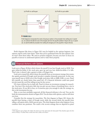
Chapter 20 Understanding Options 503
Investors regularly trade options on common stocks.2
For example, Table 20.1 reproduces
quotes for options on the stock of Google. You can see that there are two types of option—
calls and puts. We explain each in turn.
Call Options and Position Diagrams
A call option gives its owner the right to buy stock at a specified exercise or strike price on
or before a specified maturity date. If the option can be exercised only at maturity, it is
conventionally known as a European call; in other cases (such as the Google options shown
in Table 20.1), the option can be exercised on or at any time before maturity, and it is then
known as an American call.
The third column of Table 20.1 sets out the prices of Google call options with dif-
ferent exercise prices and exercise dates. Look at the quotes for options maturing in
2
The two principal options exchanges in the United States are the International Securities Exchange (ISE) and the Chicago Board
Options Exchange (CBOE).
20-1 Calls, Puts, and Shares
● ● ● ● ●
Once the project is no longer profitable, the company
will cut its losses and exercise its option to abandon the
project. Some projects have higher abandonment value
than others. Those that use standardized equipment
may offer a valuable abandonment option. Others may
actually cost money to discontinue. For example, it is
very costly to decommission an offshore oil platform.
We took a peek at investment options in Chapter 10,
and we showed there how to use decision trees to analyze
a pharmaceutical company’s options to discontinue trials
of a new drug. In Chapter 22 we take a more thorough
look at these real options.
The other important reason why financial managers
need to understand options is that they are often tacked
on to an issue of corporate securities and so provide
the investor or the company with the flexibility to change
the terms of the issue. For example, in Chapter 24
we show how warrants or convertibles give their holders
an option to buy common stock in exchange for cash
or bonds.
In fact, we see in Chapter 23 that whenever a
company borrows, it gains an option to walk away from
its debts and surrender its assets to the bondholders.
If the value of the company’s assets is less than the
amount of the debt, the company will choose to default
on the payment and the bondholders will get to keep
the company’s assets. Thus, when the firm borrows,
the lender effectively acquires the company and the
shareholders obtain the option to buy it back by paying
off the debt. This is an extremely important insight. It
means that anything that we can learn about traded
options applies equally to corporate liabilities.
In this chapter we use traded stock options to
explain how options work, but we hope that our brief
survey has convinced you that the interest of financial
managers in options goes far beyond traded stock
options. That is why we are asking you to invest here to
acquire several important ideas for use later.
If you are unfamiliar with the wonderful world of
options, it may seem baffling on first encounter. We
therefore divide this chapter into three bite-sized pieces.
Our first task is to introduce you to call and put options
and to show you how the payoff on these options
depends on the price of the underlying asset. We then
show how financial alchemists can combine options to
produce a variety of interesting strategies.
We conclude the chapter by identifying the variables
that determine option values. There you encounter some
surprising and counterintuitive effects. For example,
investors are used to thinking that increased risk
reduces present value. But for options it is the other way
around.

confirming pages
504 Part Six Options
December 2008. The first entry says that for $78.90 you could acquire an option to buy one
share3
of Google stock for $370 on or before December 2008. Moving down to the next
row, you can see that an option to buy for $30 more ($400 vs. $370) costs $20.25 less, that
is $58.65. In general, the value of a call option goes down as the exercise price goes up.
Now look at the quotes for options maturing in March 2009 and January 2010. Notice
how the option price increases as option maturity is extended. For example, at an exercise
price of $430, the December 2008 call option costs $41.75, the March 2009 option costs
$54.35, and the January 2010 option costs $85.05.
In Chapter 13 we met Louis Bachelier, who in 1900 first suggested that security prices
follow a random walk. Bachelier also devised a very convenient shorthand to illustrate the
effects of investing in different options. We use this shorthand to compare a call option
and a put option on Google stock.
The position diagram in Figure 20.1(a) shows the possible consequences of investing in
Google March 2009 call options with an exercise price of $430 (boldfaced in Table 20.1).
The outcome from investing in Google calls depends on what happens to the stock price.
If the stock price at the end of this six-month period turns out to be less than the $430
exercise price, nobody will pay $430 to obtain the share via the call option. Your call will in
that case be valueless, and you will throw it away. On the other hand, if the stock price turns
out to be greater than $430, it will pay to exercise your option to buy the share. In this case,
when the call expires, it will be worth the market price of the share minus the $430 that you
must pay to acquire it. For example, suppose that the price of Google stock rises to $500.
Your call will then be worth $500 Ϫ $430 ϭ $70. That is your payoff, but of course it is not
all profit. Table 20.1 shows that you had to pay $54.35 to buy the call.
3
You can’t actually buy an option on a single share. Trades are in multiples of 100. The minimum order would be for 100 options
on 100 Google shares.
Maturity Date
Exercise
Price
Price of Call
Option
Price of Put
Option
December 2008 $370 $ 78.90 $16.45
400 58.65 26.10
430 41.75 38.90
460 28.05 55.45
490 17.85 75.45
March 2009 $370 $ 90.20 $25.05
400 70.80 35.65
430 54.35 48.55
460 39.85 64.10
490 28.75 83.20
January 2010*
$370 $116.90 $42.55
400 100.00 54.75
430 85.05 69.85
460 71.60 86.00
490 59.90 103.70
◗ TABLE 20.1
Selected prices of
put and call options
on Google stock in
September 2008, when
the closing stock price
was $430.
* Long-term options are
called “LEAPS.”
Source: Yahoo! Finance,
http://finance.yahoo.com.
Reproduced with permission
of Yahoo! Inc. © 2008 by
Yahoo! Inc. Yahoo! and
the Yahoo! logo are
trademarks of Yahoo! Inc.

confirming pages
Put Options
Now let us look at the Google put options in the right-hand column of Table 20.1. Whereas
a call option gives you the right to buy a share for a specified exercise price, a put gives you
the right to sell the share. For example, the boldfaced entry in the right-hand column of
Table 20.1 shows that for $48.55 you could acquire an option to sell Google stock for a
price of $430 anytime before March 2009. The circumstances in which the put turns out
to be profitable are just the opposite of those in which the call is profitable. You can see
this from the position diagram in Figure 20.1(b). If Google’s share price immediately before
expiration turns out to be greater than $430, you won’t want to sell stock at that price. You
would do better to sell the share in the market, and your put option will be worthless.
Conversely, if the share price turns out to be less than $430, it will pay to buy stock at the
low price and then take advantage of the option to sell it for $430. In this case, the value
of the put option on the exercise date is the difference between the $430 proceeds of the
sale and the market price of the share. For example, if the share is worth $340, the put is
worth $90:
Value of put option at expiration 5 exercise price 2 market price of the share
5 $430 2 $340 5 $90
Selling Calls, Puts, and Shares
Let us now look at the position of an investor who sells these investments. If you sell, or
“write,” a call, you promise to deliver shares if asked to do so by the call buyer. In other
words, the buyer’s asset is the seller’s liability. If the share price is below the exercise price
when the option matures, the buyer will not exercise the call and the seller’s liability will
be zero. If it rises above the exercise price, the buyer will exercise and the seller must give
up the shares. The seller loses the difference between the share price and the exercise price
received from the buyer. Notice that it is the buyer who always has the option to exercise;
option sellers simply do as they are told.
$430
(a)
$430
(b)
$430 $430
Value of
call
Value of
put
Share
price
Share
price0 0
◗ FIGURE 20.1
Position diagrams show how payoffs to owners of Google calls and puts (shown by the colored lines) depend
on the share price. (a) Result of buying Google call exercisable at $430. (b) Result of buying Google put
exercisable at $430.

confirming pages
Suppose that the price of Google stock turns out to be $500, which is above the option’s
exercise price of $430. In this case the buyer will exercise the call. The seller is forced to sell
stock worth $500 for only $430 and so has a payoff of Ϫ$70.4
Of course, that $70 loss is the
buyer’s gain. Figure 20.2(a) shows how the payoffs to the seller of the Google call option
vary with the stock price. Notice that for every dollar the buyer makes, the seller loses a
dollar. Figure 20.2(a) is just Figure 20.1(a) drawn upside down.
In just the same way we can depict the position of an investor who sells, or writes, a put
by standing Figure 20.1(b) on its head. The seller of the put has agreed to pay $430 for the
share if the buyer of the put should request it. Clearly the seller will be safe as long as the
share price remains above $430 but will lose money if the share price falls below this figure.
The worst thing that can happen is that the stock becomes worthless. The seller would then
be obliged to pay $430 for a stock worth $0. The payoff to the option position would be
Ϫ$430.
Position Diagrams Are Not Profit Diagrams
Position diagrams show only the payoffs at option exercise; they do not account for the
initial cost of buying the option or the initial proceeds from selling it.
This is a common point of confusion. For example, the position diagram in Figure 20.1(a)
makes purchase of a call look like a sure thing—the payoff is at worst zero, with plenty of
upside if Google’s stock price goes above $430 by March 2009. But compare the profit dia-
gram in Figure 20.3(a), which subtracts the $54.35 cost of the call in September 2008 from
the payoff at maturity. The call buyer loses money at all share prices less than $430 ϩ 54.35
ϭ $484.35. Take another example: The position diagram in Figure 20.2(b) makes selling
a put look like a sure loss—the best payoff is zero. But the profit diagram in Figure 20.3(b),
which recognizes the $48.55 received by the seller, shows that the seller gains at all prices
above $430 Ϫ 48.55 ϭ $381.45.5
4
The seller has some consolation, for he or she was paid $54.35 in September for selling the call.
5
The fact that you have made a profit on your position is not necessarily a cause for rejoicing. The profit needs to compensate
you for the time value of money and the risk that you took.
$430
(a)
$430
(b)
Ϫ$430 Ϫ$430
0 0
Share
price
Share
price
Value of call
seller's position
Value of put
seller's position
◗ FIGURE 20.2
Payoffs to sellers of Google calls and puts (shown by the colored lines) depend on the share price. (a) Result
of selling Google call exercisable at $430. (b) Result of selling Google put exercisable at $430.

confirming pages
Profit diagrams like those in Figure 20.3 may be helpful to the options beginner, but
options experts rarely draw them.6
Now that you’ve graduated from the first options class
we won’t draw them either. We stick to position diagrams, because you have to focus on
payoffs at exercise to understand options and to value them properly.
Look now at Figure 20.4(a), which shows the payoff if you buy Google stock at $430. You
gain dollar-for-dollar if the stock price goes up and you lose dollar-for-dollar if it falls.
That’s trite; it doesn’t take a genius to draw a 45-degree line.
Look now at panel (b), which shows the payoffs from an investment strategy that retains
the upside potential of Google stock but gives complete downside protection. In this case
your payoff stays at $430 even if the Google stock price falls to $400, $100, or zero. Panel
(b)’s payoffs are clearly better than panel (a)’s. If a financial alchemist could turn panel
(a) into panel (b), you’d be willing to pay for the service.
Of course alchemy has its dark side. Panel (c) shows an investment strategy for masoch-
ists. You lose if the stock price falls, but you give up any chance of profiting from a rise in
the stock price. If you like to lose, or if someone pays you enough to take the strategy on,
this is the investment for you.
Now, as you have probably suspected, all this financial alchemy is for real. You can do
both the transmutations shown in Figure 20.4. You do them with options, and we will show
you how.
Consider first the strategy for masochists. The first diagram in Figure 20.5 shows the
payoffs from buying a share of Google stock, while the second shows the payoffs from
selling a call option with a $430 exercise price. The third diagram shows what happens if you
combine these two positions. The result is the no-win strategy that we depicted in panel
6
Profit diagrams such as Figure 20.3 deduct the initial cost of the option from the final payoff. They therefore ignore the first
lesson of finance—“A dollar today is worth more than a dollar in the future.”
20-2 Financial Alchemy with Options
$430
(a) Profit to call buyer (b) Profit to put seller
–$54.35
0
$48.55Share
price Share
priceBreakeven
is $484.35
$430
0
Breakeven
is $381.45
◗ FIGURE 20.3
Profit diagrams incorporate the costs of buying an option or the proceeds from selling one. In panel
(a), we subtract the $54.35 cost of the Google call from the payoffs plotted in Figure 20.1(a). In panel
(b), we add the $48.55 proceeds from selling the Google put to the payoffs in Figure 20.2(b).

confirming pages
Lose
if stock
price falls
Lose
if stock
price falls
Win if stock
price rises
Your
payoff
Future
stock
price
$430
(a)
Win if stock
price rises
Your
payoff
Future
stock
price
$430
(b)
Protected on
downside
No upside
Your
payoff
Future
stock
price
$430
(c)
◗ FIGURE 20.4
Payoffs at the end of six months to three investment strategies for Google stock. (a) You buy one share for
$430. (b) No downside. If stock price falls, your payoff stays at $430. (c) A strategy for masochists? You
lose if stock price falls, but you don’t gain if it rises.
(c) of Figure 20.4. You lose if the stock price declines below $430, but, if the stock price rises
above $430, the owner of the call will demand that you hand over your stock for the $430
exercise price. So you lose on the downside and give up any chance of a profit. That’s the
bad news. The good news is that you get paid for taking on this liability. In September 2009
you would have been paid $54.35, the price of a six-month call option.
Now, we’ll create the downside protection shown in Figure 20.4(b). Look at row 1 of
Figure 20.6. The first diagram again shows the payoff from buying a share of Google stock,
while the next diagram in row 1 shows the payoffs from buying a Google put option with
an exercise price of $430. The third diagram shows the effect of combining these two posi-
tions. You can see that, if Google’s stock price rises above $430, your put option is value-
less, so you simply receive the gains from your investment in the share. However, if the
stock price falls below $430, you can exercise your put option and sell your stock for $430.
Thus, by adding a put option to your investment in the stock, you have protected yourself
against loss.7
This is the strategy that we depicted in panel (b) of Figure 20.4. Of course,
7
This combination of a stock and a put option is known as a protective put.

confirming pages
there is no gain without pain. The cost of insuring yourself against loss is the amount that
you pay for a put option on Google stock with an exercise price of $430. In September 2008
the price of this put was $48.55. This was the going rate for financial alchemists.
We have just seen how put options can be used to provide downside protection. We
now show you how call options can be used to get the same result. This is illustrated in
row 2 of Figure 20.6. The first diagram shows the payoff from placing the present value of
$430 in a bank deposit. Regardless of what happens to the price of Google stock, your bank
deposit will pay off $430. The second diagram in row 2 shows the payoff from a call option
on Google stock with an exercise price of $430, and the third diagram shows the effect of
combining these two positions. Notice that, if the price of Google stock falls, your call is
worthless, but you still have your $430 in the bank. For every dollar that Google stock price
rises above $430, your investment in the call option pays off an extra dollar. For example,
if the stock price rises to $500, you will have $430 in the bank and a call worth $70. Thus
you participate fully in any rise in the price of the stock, while being fully protected against
any fall. So we have just found another way to provide the downside protection depicted
in panel (b) of Figure 20.4.
These two rows of Figure 20.6 tell us something about the relationship between a call
option and a put option. Regardless of the future stock price, both investment strategies
provide identical payoffs. In other words, if you buy the share and a put option to sell it for
$430, you receive the same payoff as from buying a call option and setting enough money
aside to pay the $430 exercise price. Therefore, if you are committed to holding the two
packages until the options expire, the two packages should sell for the same price today.
This gives us a fundamental relationship for European options:
Value of call 1 present value of exercise price 5 value of put 1 share price
To repeat, this relationship holds because the payoff of
Buy call, invest present value of exercise price in safe asset8
is identical to the payoff from
Buy put, buy share
8
The present value is calculated at the risk-free rate of interest. It is the amount that you would have to invest today in a bank
deposit or Treasury bills to realize the exercise price on the option’s expiration date.
$430
Buy share
Your
payoff
Future
stock
price
$430
Sell call
Your
payoff
Future
stock
price
$430
No upside
Your
payoff
Future
stock
price
+ =
◗ FIGURE 20.5
You can use options to create a strategy where you lose if the stock price falls but do not gain if it rises (strategy [c] in Figure 20.4).

confirming pages
This basic relationship among share price, call and put values, and the present value of the
exercise price is called put–call parity.9
Put–call parity can be expressed in several ways. Each expression implies two investment
strategies that give identical results. For example, suppose that you want to solve for the
value of a put. You simply need to twist the put–call parity formula around to give
Value of put 5 value of call 1 present value of exercise price 2 share price
From this expression you can deduce that
Buy put
is identical to
Buy call, invest present value of exercise price in safe asset, sell share
In other words, if puts are not available, you can get exactly the same payoff by buying calls,
putting cash in the bank, and selling shares.
9
Put–call parity holds only if you are committed to holding the options until the final exercise date. It therefore does not hold for
American options, which you can exercise before the final date. We discuss possible reasons for early exercise in Chapter 21. Also
if the stock makes a dividend payment before the final exercise date, you need to recognize that the investor who buys the call
misses out on this dividend. In this case the relationship is
Value of call 1 present value of exercise price 5 value of put 1 share price 2 present value of dividend
$430
Buy share
Your
payoff
Future
stock
price
$430
Buy put
Your
payoff
Future
stock
price
$430
Downside
protection
Downside
protection
Your
payoff
Future
stock
price
+ =
$430
$430
Bank deposit paying $430
Your
payoff
Future
stock
price
$430
Buy call
Your
payoff
Future
stock
price
$430
Your
payoff
Future
stock
price
+ =
◗ FIGURE 20.6
Each row in the figure shows a different way to create a strategy where you gain if the stock price rises but are protected on the
downside (strategy [b] in Figure 20.4).

confirming pages
If you find this difficult to believe, look at Figure 20.7, which shows the possible pay-
offs from each position. The diagram on the left shows the payoffs from a call option on
Google stock with an exercise price of $430. The second diagram shows the payoffs from
placing the present value of $430 in the bank. Regardless of what happens to the share
price, this investment will pay off $430. The third diagram shows the payoffs from selling
Google stock. When you sell a share that you don’t own, you have a liability—you must
sometime buy it back. As they say on Wall Street:
He who sells what isn’t his’n
Buys it back or goes to pris’n
Therefore the best that can happen to you is that the share price falls to zero. In that case it
costs you nothing to buy the share back. But for every extra dollar on the future share price,
you will need to spend an extra dollar to buy the share. The final diagram in Figure 20.7 shows
that the total payoff from these three positions is the same as if you had bought a put option.
For example, suppose that when the option matures the stock price is $400. Your call will be
worthless, your bank deposit will be worth $430, and it will cost you $400 to repurchase the
share. Your total payoff is 0 ϩ 430 Ϫ 400 ϭ $30, exactly the same as the payoff from the put.
If two investments offer identical payoffs, then they should sell for the same price today.
If the law of one price is violated, you have a potential arbitrage opportunity. So let’s
check whether there are any arbitrage profits to be made from our Google calls and puts.
In September 2008 the price of a six-month call with a $430 exercise price was $54.35, the
interest rate was about 3%, and the price of Google stock was $430. Therefore the cost of
a homemade put was:
Buy call ϩ present value of exercise price Ϫ share price ϭ cost of homemade put
54.35 ϩ 430/1.03.5
Ϫ 430 ϭ 48.04
This is almost exactly the same as it would have cost you to buy a put directly.
$430
$0
Your
payoff
Buy call
+
Your
payoff
Bank deposit
paying $430 +
Your
payoff
Sell stock
$430
=
Your
payoff
Buy put
◗ FIGURE 20.7
A strategy of buying a call, depositing the present value of the exercise price in the bank, and selling the stock is equivalent to
buying a put.

confirming pages
Spotting the Option
Options rarely come with a large label attached. Often the trickiest part of the problem is
to identify the option. When you are not sure whether you are dealing with a put or a call
or a complicated blend of the two, it is a good precaution to draw a position diagram. Here
is an example.
The Flatiron and Mangle Corporation has offered its president, Ms. Higden, the follow-
ing incentive scheme: At the end of the year Ms. Higden will be paid a bonus of $50,000
for every dollar that the price of Flatiron stock exceeds its current figure of $120. However,
the maximum bonus that she can receive is set at $2 million.
You can think of Ms. Higden as owning 50,000 tickets, each of which pays nothing if
the stock price fails to beat $120. The value of each ticket then rises by $1 for each dollar
rise in the stock price up to the maximum of $2,000,000/50,000 ϭ $40. Figure 20.8 shows
the payoffs from just one of these tickets. The payoffs are not the same as those of the
simple put and call options that we drew in Figure 20.1, but it is possible to find a combi-
nation of options that exactly replicates Figure 20.8. Before going on to read the answer,
see if you can spot it yourself. (If you are someone who enjoys puzzles of the make-a-
triangle-from-just-two-matchsticks type, this one should be a walkover.)
The answer is in Figure 20.9. The solid black line represents the purchase of a call option
with an exercise price of $120, and the dotted line shows the sale of another call option with
$120
$160
$40
Payoff
Stock
price
◗ FIGURE 20.9
The solid black line shows
the payoff from buying a
call with an exercise price
of $120. The dotted line
shows the sale of a call
with an exercise price of
$160. The combined pur-
chase and sale (shown by
the colored line) is identi-
cal to one of Ms. Higden’s
“tickets.”
$120 $160
$40
Payoff
Stock
price
◗ FIGURE 20.8
The payoff from one of
Ms. Higden’s “tickets”
depends on Flatiron’s
stock price.

confirming pages
an exercise price of $160. The colored line shows the payoffs from a combination of the
purchase and the sale—exactly the same as the payoffs from one of Ms. Higden’s tickets.
Thus, if we wish to know how much the incentive scheme is costing the company, we
need to calculate the difference between the value of 50,000 call options with an exercise
price of $120 and the value of 50,000 calls with an exercise price of $160.
We could have made the incentive scheme depend in a much more complicated way on
the stock price. For example, the bonus could peak at $2 million and then fall steadily back
to zero as the stock price climbs above $160.10
You could still have represented this scheme
as a combination of options. In fact, we can state a general theorem:
Any set of contingent payoffs—that is, payoffs that depend on the value of some other
asset—can be constructed with a mixture of simple options on that asset.
In other words, you can create any position diagram—with as many ups and downs or peaks
and valleys as your imagination allows—by buying or selling the right combinations of puts
and calls with different exercise prices.11
Finance pros often talk about financial engineering, which is the practice of packaging
different investments to create new tailor-made instruments. Perhaps a German company
would like to set a minimum and maximum cost at which it can buy dollars in six-months’
time. Or perhaps an oil company would like to pay a lower rate of interest on its debt if the
price of oil falls. Options provide the building blocks that financial engineers use to create
these interesting payoff structures.
So far we have said nothing about how the market value of an option is determined. We do
know what an option is worth when it matures, however. Consider, for instance, our earlier
example of an option to buy Google stock at $430. If Google’s stock price is below $430
on the exercise date, the call will be worthless; if the stock price is above $430, the call will
be worth $430 less than the value of the stock. This relationship is depicted by the heavy,
lower line in Figure 20.10.
Even before maturity the price of the option can never remain below the heavy, lower-
bound line in Figure 20.10. For example, if our option were priced at $10 and the stock
were priced at $460, it would pay any investor to sell the stock and then buy it back by
purchasing the option and exercising it for an additional $430. That would give an arbitrage
opportunity with a profit of $20. The demand for options from investors seeking to exploit
this opportunity would quickly force the option price up, at least to the heavy line in the
figure. For options that still have some time to run, the heavy line is therefore a lower bound
on the market price of the option. Option geeks express the same idea more concisely when
they write Lower Bound ϭ Max(stock price Ϫ exercise price, 0).
The diagonal line in Figure 20.10 is the upper bound to the option price. Why? Because the
option cannot give a higher ultimate payoff than the stock. If at the option’s expiration the stock
price ends up above the exercise price, the option is worth the stock price less the exercise price.
10
This is not as nutty a bonus scheme as it may sound. Maybe Ms. Higden’s hard work can lift the value of the stock by so
much and the only way she can hope to increase it further is by taking on extra risk. You can deter her from doing this by
making her bonus start to decline beyond some point. Too bad that the bonus schemes for some bank CEOs did not contain
this feature.
11
In some cases you may also have to borrow or lend money to generate a position diagram with your desired pattern. Lending
raises the payoff line in position diagrams, as in the bottom row of Figure 20.6. Borrowing lowers the payoff line.
20-3 What Determines Option Values?

confirming pages
If the stock price ends up below the exercise price, the option is worthless, but the stock’s owner
still has a valuable security. For example, if the option’s exercise price is $430, then the extra
dollar returns realized by stockholders are shown in the following table:
Stock
Payoff
Option
Payoff
Extra Payoff from
Holding Stock Instead
of Option
Option exercised (stock
price greater than $430) Stock price Stock price Ϫ430 $430
Option expires unexercised
(stock price less than or
equal to $430) Stock price 0 Stock price
If the stock and the option have the same price, everyone will rush to sell the option
and buy the stock. Therefore, the option price must be somewhere in the shaded region of
Figure 20.10. In fact, it will lie on a curved, upward-sloping line like the dashed curve shown
in the figure. This line begins its travels where the upper and lower bounds meet (at zero).
Then it rises, gradually becoming parallel to the upward-sloping part of the lower bound.
But let us look more carefully at the shape and location of the dashed line. Three points,
A, B, and C, are marked on the dashed line. As we explain each point you will see why the
option price has to behave as the dashed line predicts.
Point A When the stock is worthless, the option is worthless. A stock price of zero means that
there is no possibility the stock will ever have any future value.12
If so, the option is sure to
expire unexercised and worthless, and it is worthless today.
That brings us to our first important point about option value:
The value of an option increases as stock price increases, if the exercise price is held constant.
That should be no surprise. Owners of call options clearly hope for the stock price to
rise and are happy when it does.
Point B When the stock price becomes large, the option price approaches the stock price less the
present value of the exercise price. Notice that the dashed line representing the option price
12
If a stock can be worth something in the future, then investors will pay something for it today, although possibly a very small
amount.
Lower bound:
Value of call
equals payoff
if exercised
immediately
Upper bound:
Value of call
equals share
price
C
B
Value of call
Exercise price
Share price
A
◗ FIGURE 20.10
Value of a call before its
expiration date (dashed
line). The value depends
on the stock price. It is
always worth more than
its value if exercised
now (heavy line). It is
never worth more than
the stock price itself.

confirming pages
in Figure 20.10 eventually becomes parallel to the ascending heavy line representing the
lower bound on the option price. The reason is as follows: The higher the stock price, the
higher is the probability that the option will eventually be exercised. If the stock price is
high enough, exercise becomes a virtual certainty; the probability that the stock price will
fall below the exercise price before the option expires becomes trivially small.
If you own an option that you know will be exchanged for a share of stock, you effectively
own the stock now. The only difference is that you don’t have to pay for the stock (by hand-
ing over the exercise price) until later, when formal exercise occurs. In these circumstances,
buying the call is equivalent to buying the stock but financing part of the purchase by bor-
rowing. The amount implicitly borrowed is the present value of the exercise price. The value
of the call is therefore equal to the stock price less the present value of the exercise price.
This brings us to another important point about options. Investors who acquire stock by
way of a call option are buying on credit. They pay the purchase price of the option today,
but they do not pay the exercise price until they actually take up the option. The delay in
payment is particularly valuable if interest rates are high and the option has a long maturity.
Thus, the value of an option increases with both the rate of interest and the time to
maturity.
Point C The option price always exceeds its minimum value (except when stock price is zero).
We have seen that the dashed and heavy lines in Figure 20.10 coincide when stock price
is zero (point A), but elsewhere the lines diverge; that is, the option price must exceed the
minimum value given by the heavy line. The reason for this can be understood by examin-
ing point C.
At point C, the stock price exactly equals the exercise price. The option is therefore
worthless if exercised today. However, suppose that the option will not expire until three
months hence. Of course we do not know what the stock price will be at the expiration
date. There is roughly a 50% chance that it will be higher than the exercise price and a 50%
chance that it will be lower. The possible payoffs to the option are therefore:
Outcome Payoff
Stock price rises
(50% probability)
Stock price less exercise price
(option is exercised)
Stock price falls
(50% probability)
Zero
(option expires worthless)
If there is a positive probability of a positive payoff, and if the worst payoff is zero, then the
option must be valuable. That means the option price at point C exceeds its lower bound,
which at point C is zero. In general, the option prices will exceed their lower-bound values
as long as there is time left before expiration.
One of the most important determinants of the height of the dashed curve (i.e., of the
difference between actual and lower-bound value) is the likelihood of substantial move-
ments in the stock price. An option on a stock whose price is unlikely to change by more
than 1% or 2% is not worth much; an option on a stock whose price may halve or double
is very valuable.
As an option holder, you gain from volatility because the payoffs are not symmetric. If
the stock price falls below the exercise price, your call option will be worthless, regardless
of whether the shortfall is a few cents or many dollars. On the other hand, for every dollar
that the stock price rises above the exercise price, your call will be worth an extra dollar.
Therefore, the option holder gains from the increased volatility on the upside, but does not
lose on the downside.
A simple example may help to illustrate the point. Consider two stocks, X and Y, each
of which is priced at $100. The only difference is that the outlook for Y is much less easy

confirming pages
to predict. There is a 50% chance that the price of Y will rise to $150 and a similar chance
that it will fall to $70. By contrast, there is a 50-50 chance that the price of X will either rise
to $130 or fall to $90.
Suppose that you are offered a call option on each of these stocks with an exercise price
of $100. The following table compares the possible payoffs from these options:
Stock Price Falls Stock Price Rises
Payoff from option on X $0 $130 Ϫ $100 ϭ $30
Payoff from option on Y $0 $150 Ϫ $100 ϭ $50
In both cases there is a 50% chance that the stock price will decline and make the option
worthless but, if the stock price rises, the option on Y will give the larger payoff. Since the
chance of a zero payoff is the same, the option on Y is worth more than the option on X.
Of course, in practice future stock prices may take on a range of different values. We
have recognized this in Figure 20.11, where the uncertain outlook for Y’s stock price shows
up in the wider probability distribution of future prices.13
The greater spread of outcomes
13
Figure 20.11 continues to assume that the exercise price on both options is equal to the current stock price. This is not a neces-
sary assumption. Also in drawing Figure 20.11 we have assumed that the distribution of stock prices is symmetric. This also is not
a necessary assumption, and we will look more carefully at the distribution of stock prices in the next chapter.
Probability
distribution of
future price of
firm X's shares
Payoff to call
option on firm
X's shares
Payoff to
option on X
Firm X
share priceExercise price
(a)
Probability
distribution of
future price of
firm Y's shares
Payoff to call
option on firm
Y's shares
Payoff to
option on Y
Firm Y
share priceExercise price
(b)
◗ FIGURE 20.11
Call options on the
shares of (a) firm X
and (b) firm Y. In each
case, the current share
price equals the exercise
price, so each option
has a 50% chance of
ending up worthless (if
the share price falls) and
a 50% chance of ending
up “in the money” (if
the share price rises).
However, the chance of
a large payoff is greater
for the option on firm
Y’s shares because
Y’s stock price is more
volatile and therefore has
more upside potential.

for stock Y again provides more upside potential and therefore increases the chance of a
large payoff on the option.
Figure 20.12 shows how volatility affects the value of an option. The upper curved line
depicts the value of the Google call option assuming that Google’s stock price, like that
of stock Y, is highly variable. The lower curved line assumes a lower (and more realistic)
degree of volatility.14
The probability of large stock price changes during the remaining life of an option
depends on two things: (1) the variance (i.e., volatility) of the stock price per period and
(2) the number of periods until the option expires. If there are t remaining periods, and the
variance per period is ␴2
, the value of the option should depend on cumulative variability
␴2
t.15
Other things equal, you would like to hold an option on a volatile stock (high ␴2
).
Given volatility, you would like to hold an option with a long life ahead of it (large t).
Thus the value of an option increases with both the volatility of the share price and the
time to maturity.
It’s a rare person who can keep all these properties straight at first reading. Therefore, we
have summed them up in Table 20.2.
Risk and Option Values
In most financial settings, risk is a bad thing; you have to be paid to bear it. Investors in
risky (high-beta) stocks demand higher expected rates of return. High-risk capital invest-
ment projects have correspondingly high costs of capital and have to beat higher hurdle
rates to achieve positive NPV.
14
The option values shown in Figure 20.12 were calculated by using the Black-Scholes option-valuation model. We explain this
model in Chapter 21 and use it to value the Google option.
15
Here is an intuitive explanation: If the stock price follows a random walk (see Section 13-2), successive price changes are sta-
tistically independent. The cumulative price change before expiration is the sum of t random variables. The variance of a sum of
independent random variables is the sum of the variances of those variables. Thus, if ␴2
is the variance of the daily price change,
and there are t days until expiration, the variance of the cumulative price change is ␴2
t.
0
100
1000 200 300 400 500 600
200
300
400
500
600
Exercise price = $430
Upper
bound
Values of Google call option
Share price
Lower bound
◗ FIGURE 20.12
How the value of the
Google call option
increases with the
volatility of the stock price.
Each of the curved lines
shows the value of the
option for different initial
stock prices. The only dif-
ference is that the upper
line assumes a much
higher level of uncertainty
about Google’s future
stock price.
Visit us at
www.mhhe.com/bma

● ● ● ● ●
confirming pages
EXAMPLE 20.1 ● Volatility and Executive Stock Options
For options it’s the other way around. As we have just seen, options written on volatile
assets are worth more than options written on safe assets. If you can understand and remem-
ber that one fact about options, you’ve come a long way.
1. If there is an
increase in:
The change in the call
option price is:
Stock price (P) Positive
Exercise price (EX) Negative
Interest rate (rf) Positive*
Time to expiration (t) Positive
Volatility of stock price (␴) Positive*
2. Other properties of call options:
a. Upper bound. The option price is always less than the stock price.
b. Lower bound. The call price never falls below the payoff to immediate
exercise (P Ϫ EX or zero, whichever is larger).
c. If the stock is worthless, the call is worthless.
d. As the stock price becomes very large, the call price approaches the stock price less the present value of the
exercise price.
◗ TABLE 20.2
What the price of a call
option depends on.
* The direct effect of
increases in rf or ␴ on option
price, given the stock price.
There may also be indirect
effects. For example, an
increase in rf could reduce
stock price P. This in turn
could affect option price.
Establishment Industries Digital Organics
Number of options 100,000 100,000
Exercise price $25 $25
Maturity 5 years 5 years
Current stock price $22 $22
Stock price volatility
(standard deviation
of return) 24% 36%
◗ TABLE 20.3
Which package of
executive stock options
would you choose?
The package offered by
Digital Organics is more
valuable, because the
volatility of that com-
pany’s stock is higher.
Suppose you have to choose between two job offers, as CFO of either Establishment
Industries or Digital Organics. Establishment Industries’ compensation package includes a
grant of the stock options described on the left side of Table 20.3. You demand a similar
package from Digital Organics, and they comply. In fact they match the Establishment
Industries options in every respect, as you can see on the right side of Table 20.3. (The two
companies’ current stock prices just happen to be the same.) The only difference is that
Digital Organics’ stock is 50% more volatile than Establishment Industries’ stock (36%
annual standard deviation vs. 24% for Establishment Industries).
If your job choice hinges on the value of the executive stock options, you should take
the Digital Organics offer. The Digital Organics options are written on the more volatile
asset and therefore are worth more.
We value the two stock-option packages in the next chapter.

confirming pages
If you have managed to reach this point, you are probably in need of a rest and a stiff gin
and tonic. So we will summarize what we have learned so far and take up the subject of options
again in the next chapter when you are rested (or drunk).
There are two types of option. An American call is an option to buy an asset at a specified
exercise price on or before a specified maturity date. Similarly, an American put is an option to
sell the asset at a specified price on or before a specified date. European calls and puts are exactly
the same except that they cannot be exercised before the specified maturity date. Calls and puts
are the basic building blocks that can be combined to give any pattern of payoffs.
What determines the value of a call option? Common sense tells us that it ought to depend
on three things:
1. To exercise an option you have to pay the exercise price. Other things being equal, the less
you are obliged to pay, the better. Therefore, the value of a call option increases with the ratio
of the asset price to the exercise price.
2. You do not have to pay the exercise price until you decide to exercise the option. Therefore,
a call option gives you a free loan. The higher the rate of interest and the longer the time to
maturity, the more this free loan is worth. So the value of a call option increases with the
interest rate and time to maturity.
3. If the price of the asset falls short of the exercise price, you won’t exercise the call option.
You will, therefore, lose 100% of your investment in the option no matter how far the asset
depreciates below the exercise price. On the other hand, the more the price rises above the
exercise price, the more profit you will make. Therefore the option holder does not lose
from increased volatility if things go wrong, but gains if they go right. The value of an
option increases with the variance per period of the stock return multiplied by the number
of periods to maturity.
Always remember that an option written on a risky (high-variance) asset is worth more than
an option on a safe asset. It’s easy to forget, because in most other financial contexts increases
in risk reduce present value.
SUMMARY
● ● ● ● ●
See Further Readings for Chapter 21. FURTHER READING
● ● ● ● ●
BASIC
1. Complete the following passage:
A _______ option gives its owner the opportunity to buy a stock at a specified price that is
generally called the _______ price. A _______ option gives its owner the opportunity to sell
stock at a specified price. Options that can be exercised only at maturity are called _______
options.
2. Note Figure 20.13 on the next page. Match each diagram, (a) and (b), with one of the fol-
lowing positions:
• Call buyer
• Call seller
• Put buyer
• Put seller
PROBLEM SETS
● ● ● ● ●

confirming pages
3. Suppose that you hold a share of stock and a put option on that share. What is the payoff
when the option expires if (a) the stock price is below the exercise price? (b) the stock price
is above the exercise price?
4. What is put–call parity and why does it hold? Could you apply the parity formula to a call
and put with different exercise prices?
5. There is another strategy involving calls and borrowing or lending that gives the same
payoffs as the strategy described in Problem 3. What is the alternative strategy?
6. Dr. Livingstone I. Presume holds £600,000 in East African gold stocks. Bullish as he is on
gold mining, he requires absolute assurance that at least £500,000 will be available in six
months to fund an expedition. Describe two ways for Dr. Presume to achieve this goal.
There is an active market for puts and calls on East African gold stocks, and the rate of
interest is 6% per year.
7. Suppose you buy a one-year European call option on Wombat stock with an exercise price
of $100 and sell a one-year European put option with the same exercise price. The current
stock price is $100, and the interest rate is 10%.
a. Draw a position diagram showing the payoffs from your investments.
b. How much will the combined position cost you? Explain.
8. Look again at Figure 20.13. It appears that the investor in panel (b) can’t lose and the inves-
tor in panel (a) can’t win. Is that correct? Explain. (Hint: Draw a profit diagram for each
panel.)
9. What is a call option worth if (a) the stock price is zero? (b) the stock price is extremely high
relative to the exercise price?
10. How does the price of a call option respond to the following changes, other things equal?
Does the call price go up or down?
a. Stock price increases.
b. Exercise price is increased.
c. Risk-free rate increases.
d. Expiration date of the option is extended.
e. Volatility of the stock price falls.
f. Time passes, so the option’s expiration date comes closer.
11. Respond to the following statements.
a. “I’m a conservative investor. I’d much rather hold a call option on a safe stock like
Exxon Mobil than a volatile stock like Google.”
Value of investment
at maturity
Value of investment
at maturity
(a) (b)
0 Stock
price
0 Stock
price
◗ FIGURE 20.13
See Problem 2.

confirming pages
b. “I bought an American call option on Fava Farms stock, with an exercise price of $45
per share and three more months to maturity. Fava Farms’ stock has skyrocketed from
$35 to $55 per share, but I’m afraid it will fall back below $45. I’m going to lock in my
gain and exercise my call right now.”
INTERMEDIATE
12. Discuss briefly the risks and payoffs of the following positions:
a. Buy stock and a put option on the stock.
b. Buy stock.
c. Buy call.
d. Buy stock and sell call option on the stock.
e. Buy bond.
f. Buy stock, buy put, and sell call.
g. Sell put.
13. “The buyer of the call and the seller of the put both hope that the stock price will rise.
Therefore the two positions are identical.” Is the speaker correct? Illustrate with a position
diagram.
14. Pintail’s stock price is currently $200. A one-year American call option has an exercise price
of $50 and is priced at $75. How would you take advantage of this great opportunity? Now
suppose the option is a European call. What would you do?
15. It is possible to buy three-month call options and three-month puts on stock Q. Both
options have an exercise price of $60 and both are worth $10. If the interest rate is 5% a
year, what is the stock price? (Hint: Use put–call parity.)
16. In January 2009, a one-year call on the stock of Amazon.com, with an exercise price of
$45.00, sold for $19.55. The stock price was $55. The risk-free interest rate was 2.5%. How
much would you be willing to pay for a put on Amazon stock with the same maturity and
exercise price? Assume that the Amazon options are European options. (Note: Amazon
does not pay a dividend.)
17. FX Bank has succeeded in hiring ace foreign exchange trader Lucinda Cable. Her remu-
neration package reportedly includes an annual bonus of 20% of the profits that she gener-
ates in excess of $100 million. Does Ms. Cable have an option? Does it provide her with
the appropriate incentives?
18. Suppose that Mr. Colleoni borrows the present value of $100, buys a six-month put option
on stock Y with an exercise price of $150, and sells a six-month put option on Y with an
exercise price of $50.
a. Draw a position diagram showing the payoffs when the options expire.
b. Suggest two other combinations of loans, options, and the underlying stock that would
give Mr. Colleoni the same payoffs.
19. Which one of the following statements is correct?
a. Value of put ϩ present value of exercise price ϭ value of call ϩ share price.
b. Value of put ϩ share price ϭ value of call ϩ present value of exercise price.
c. Value of put Ϫ share price ϭ present value of exercise price Ϫ value of call.
d. Value of put ϩ value of call ϭ share price Ϫ present value of exercise price.
The correct statement equates the value of two investment strategies. Plot the payoffs to
each strategy as a function of the stock price. Show that the two strategies give identical
payoffs.
20. Test the formula linking put and call prices by using it to explain the relative prices of
actual traded puts and calls. (Note: The formula is exact only for European options. Most
traded puts and calls are American.)

confirming pages
21. a. If you can’t sell a share short, you can achieve exactly the same final payoff by a
combination of options and borrowing or lending. What is this combination?
b. Now work out the mixture of stock and options that gives the same final payoff as
investment in a risk-free loan.
22. The common stock of Triangular File Company is selling at $90. A 26-week call option
written on Triangular File’s stock is selling for $8. The call’s exercise price is $100. The risk-
free interest rate is 10% per year.
a. Suppose that puts on Triangular stock are not traded, but you want to buy one. How
would you do it?
b. Suppose that puts are traded. What should a 26-week put with an exercise price of $100
sell for?
23. Ms. Higden has been offered yet another incentive scheme (see Section 20-2). She will
receive a bonus of $500,000 if the stock price at the end of the year is $120 or more;
otherwise she will receive nothing. (Don’t ask why anyone should want to offer such an
arrangement. Maybe there’s some tax angle.)
a. Draw a position diagram illustrating the payoffs from such a scheme.
b. What combination of options would provide these payoffs? (Hint: You need to buy a
large number of options with one exercise price and sell a similar number with a differ-
ent exercise price.)
24. Option traders often refer to “straddles” and “butterflies.” Here is an example of each:
• Straddle: Buy call with exercise price of $100 and simultaneously buy put with exercise
price of $100.
• Butterfly: Simultaneously buy one call with exercise price of $100, sell two calls with exercise
price of $110, and buy one call with exercise price of $120.
Draw position diagrams for the straddle and butterfly, showing the payoffs from the inves-
tor’s net position. Each strategy is a bet on variability. Explain briefly the nature of each bet.
25. Look at actual trading prices of call options on stocks to check whether they behave as the
theory presented in this chapter predicts. For example,
a. Follow several options as they approach maturity. How would you expect their prices
to behave? Do they actually behave that way?
b. Compare two call options written on the same stock with the same maturity but differ-
ent exercise prices.
c. Compare two call options written on the same stock with the same exercise price but
different maturities.
26. Is it more valuable to own an option to buy a portfolio of stocks or to own a portfolio of
options to buy each of the individual stocks? Say briefly why.
27. Table 20.4 lists some prices of options on common stocks (prices are quoted to the nearest
dollar). The interest rate is 10% a year. Can you spot any mispricing? What would you do
to take advantage of it?
Stock
Time to
Exercise
(months) Exercise Price Stock Price Put Price Call Price
Drongo Corp. 6 $ 50 $80 $20 $52
Ragwort, Inc. 6 100 80 10 15
Wombat Corp. 3 40 50 7 18
6 40 50 5 17
6 50 50 8 10
◗ TABLE 20.4
Prices of options on
common stocks
(in dollars). See
Problem 27.

28. You’ve just completed a month-long study of energy markets and conclude that energy prices
will be much more volatile in the next year than historically. Assuming you’re right, what
types of option strategies should you undertake? (Note: You can buy or sell options on oil-
company stocks or on the price of future deliveries of crude oil, natural gas, fuel oil, etc.)
CHALLENGE
29. Figure 20.14 below shows some complicated position diagrams. Work out the combination
of stocks, bonds, and options that produces each of these positions.
30. Some years ago the Australian firm Bond Corporation sold a share in some land that
it owned near Rome for $110 million and as a result boosted its annual earnings by
$74 million. A television program subsequently revealed that the buyer was given a put
option to sell its share in the land back to Bond for $110 million and that Bond had paid
$20 million for a call option to repurchase the share in the land for the same price.
a. What happens if the land is worth more than $110 million when the options expire?
What if it is worth less than $110 million?
b. Use position diagrams to show the net effect of the land sale and the option transactions.
c. Assume a one-year maturity on the options. Can you deduce the interest rate?
d. The television program argued that it was misleading to record a profit on the sale of
land. What do you think?
31. Three six-month call options are traded on Hogswill stock:
Exercise Price Call Option Price
$ 90 $ 5
100 11
110 15
How would you make money by trading in Hogswill options? (Hint: Draw a graph with
the option price on the vertical axis and the ratio of stock price to exercise price on the
horizontal axis. Plot the three Hogswill options on your graph. Does this fit with what you
know about how option prices should vary with the ratio of stock price to exercise price?)
Now look in the newspaper at options with the same maturity but different exercise prices.
Can you find any money-making opportunities?
(a) (b)
(c) (d)
◗ FIGURE 20.14
Some complicated
position diagrams.
See Problem 29.

confirming pages
32. Digital Organics has 10 million outstanding shares trading at $25 per share. It also has a
large amount of debt outstanding, all coming due in one year. The debt pays interest at
8%. It has a par (face) value of $350 million, but is trading at a market value of only $280
million. The one-year risk-free interest rate is 6%.
a. Write out the put–call parity formula for Digital Organics’ stock, debt, and assets.
b. What is the value of the company’s option to default on its debt?
Go to finance.yahoo.com. Check out the delayed quotes for Google for different exercise
prices and maturities.
a. Confirm that higher exercise prices mean lower call prices and higher put prices.
b. Confirm that longer maturity means higher prices for both puts and calls.
c. Choose a Google put and call with the same exercise price and maturity. Confirm that
put–call parity holds (approximately). (Note: You will have to use an up-to-date risk-free
interest rate.)
REAL-TIME
DATA ANALYSIS
● ● ● ● ●

Fin 2 book

More Related Content

What's hot

Viewers also liked

Similar to Fin 2 book

Recently uploaded

Fin 2 book