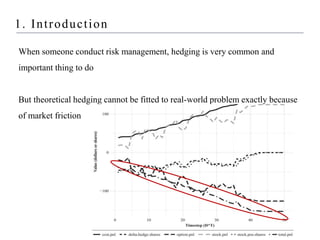
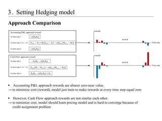
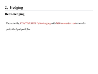
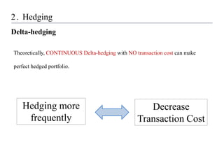
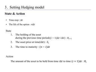
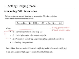
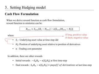
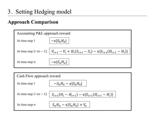
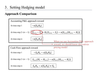
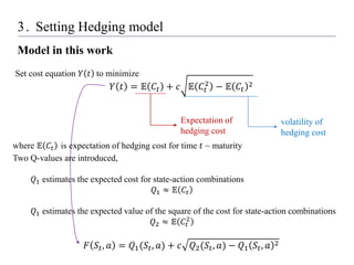
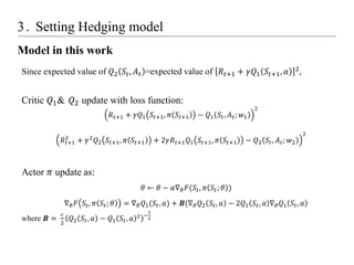
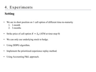
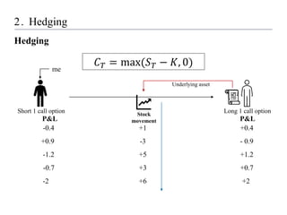
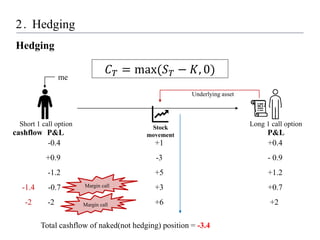
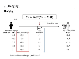
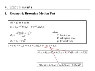
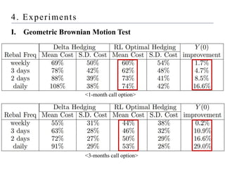
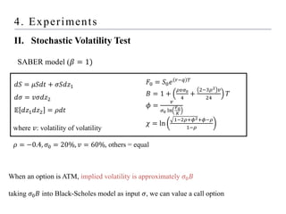
The document describes using reinforcement learning to implement hedging of derivatives. It discusses: 1) Setting up a hedging model using reinforcement learning, where the state includes the asset price and time to maturity, the action is the hedge position, and the reward minimizes hedging costs. 2) Conducting experiments hedging a short call option using the model, comparing performance under geometric Brownian motion and stochastic volatility. 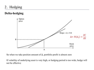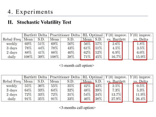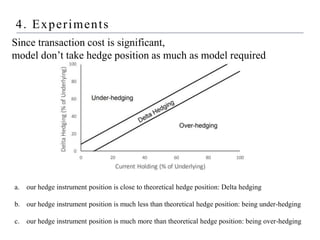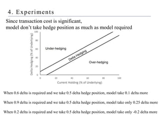3) Finding that the reinforcement learning model outperforms delta hedging strategies and achieves lower hedging costs, demonstrating the effectiveness of using reinforcement learning for hedging derivatives.

1. Deep Hedging of Derivatives Using
Reinforcement Learning
Hull et al. working paper
발표자 : 윤지상
Graduate School of Information. Yonsei Univ.
Machine Learning & Computational Finance Lab.

2. 1. Introduction
2. Hedging
3. Setting Hedging model
4. Experiments
5. Conclusion
INDEX

3. 1 Introduction

4. 1. Introduction
When someone conduct risk management, hedging is very common and
important thing to do
But theoretical hedging cannot be fitted to real-world problem exactly because
of market friction

5. 1. Introduction
Hedging is sequential optimal control task
&
RL is sequential optimal control task
Then can we implement RL to hedging task to
reduce total hedging cost?

6. 2 Hedging

7. 2. Hedging
Hedging
Short 1 call option
𝐶𝑇 = max(𝑆𝑇 − 𝐾, 0)
Long 1 call option
Underlying asset
-0.4 +0.4
+1
-3
+5
+3
+6
+0.9 - 0.9
+1.2
-1.2
+0.7
+2
-0.7
-2
P&L P&L
Stock
movement
me

8. 2. Hedging
Hedging
Short 1 call option
𝐶𝑇 = max(𝑆𝑇 − 𝐾, 0)
Long 1 call option
Underlying asset
-0.4 +0.4
+1
-3
+5
+3
+6
+0.9 - 0.9
+1.2
-1.2
+0.7
+2
-0.7
-2
Margin call
P&L P&L
Stock
movement
cashflow
-1.4
Margin call
-2
Total cashflow of naked(not hedging) position = -3.4
me

9. 2. Hedging
Hedging
Short 1 call option
𝐶𝑇 = max(𝑆𝑇 − 𝐾, 0)
Long 1 call option
Underlying asset
-0.4 +0.4
+1
-3
+5
+3
+6
+0.9 - 0.9
+1.2
-1.2
+0.7
+2
-0.7
-2
P&L P&L
Stock
movement
cashflow P&L from hedge
+0.3
-0.8
+1.4
+0.8
+1.6
Total cashflow of hedged position = 0
me

10. 2. Hedging
Hedging

11. 2. Hedging
Delta-hedging
∆= 𝑁 𝑑1 =
𝜕𝐶
𝜕𝑆
So when we take position amount of ∆, portfolio profit is almost zero
If volatility of underlying asset is very high, or hedging period is too wide, hedge will
not be effective

12. 2. Hedging
Delta-hedging
Theoretically, CONTINUOUS Delta-hedging with NO transaction cost can make
perfect hedged portfolio.

13. 2. Hedging
Delta-hedging
Theoretically, CONTINUOUS Delta-hedging with NO transaction cost can make
perfect hedged portfolio.
Hedging more
frequently
Decrease
Transaction Cost

14. 3 Setting Hedging model

15. 3. Setting Hedging model
State
1. The holding of the asset
during the previous time period((𝑖 − 1)Δ𝑡~𝑖Δ𝑡) : 𝐻𝑖−1
2. The asset price at time(𝑖Δ𝑡) : 𝑆𝑖
3. The time to maturity : (𝑛 − 𝑖)Δ𝑡
Action
The amount of the asset to be held from time 𝑖Δ𝑡 to time (𝑖 + 1)Δ𝑡 : 𝐻𝑖
State & Action
• Time-step : Δ𝑡
• The life of the option : 𝑛Δ𝑡

16. 3. Setting Hedging model
Accounting P&L formulation
𝑅𝑖+1 = 𝑉𝑖+1 − 𝑉𝑖 + 𝐻𝑖 𝑆𝑖+1 − 𝑆𝑖 − 𝜅|𝑆𝑖+1 𝐻𝑖+1 − 𝐻𝑖 |
When we derive reward function as accounting P&L formulation,
reward function to minimize can be:
where
• 𝑉𝑖 : Derivatives value at time-step 𝑖Δ𝑡
• 𝑆𝑖 : Underlying asset value at time-step 𝑖Δ𝑡
• 𝐻𝑖: Position of underlying asset relative to position of derivatives
• 𝜅 : Trading cost parameter
In addition, there are an initial reward −𝜅|𝑆0𝐻0| and final reward −𝜅|𝑆𝑛𝐻𝑛|
to set up(liquidate) the hedge position at first(last) time-step
if long, positive value
if short, negative value

17. 3. Setting Hedging model
Cash Flow Formulation
𝑅𝑖+1 = 𝑆𝑖+1 𝐻𝑖 − 𝐻𝑖+1 − 𝜅|𝑆𝑖+1 𝐻𝑖+1 − 𝐻𝑖 |
When we derive reward function as cash flow formulation,
reward function to minimize can be:
where
• 𝑆𝑖 : Underlying asset value at time-step 𝑖Δ𝑡
• 𝐻𝑖: Position of underlying asset relative to position of derivatives
• 𝜅 : Trading cost parameter
In addition, there are other rewards
• Initial rewards : −𝑆0𝐻0 − 𝜅|𝑆0𝐻0| at first time-step
• final rewards : 𝑆𝑛𝐻𝑛 − 𝜅 𝑆𝑛𝐻𝑛 + 𝑝𝑎𝑦𝑜𝑓𝑓 𝑜𝑓 𝑑𝑒𝑟𝑖𝑣𝑎𝑡𝑖𝑣𝑒𝑠 at last time-step
if long, positive value
if short, negative value

18. 3. Setting Hedging model
Approach Comparison
𝑆𝑖+1 𝐻𝑖 − 𝐻𝑖+1 − 𝜅|𝑆𝑖+1 𝐻𝑖+1 − 𝐻𝑖 |
𝑉𝑖+1 − 𝑉𝑖 + 𝐻𝑖 𝑆𝑖+1 − 𝑆𝑖 − 𝜅|𝑆𝑖+1 𝐻𝑖+1 − 𝐻𝑖 |
Accounting P&L approach reward
−𝜅|𝑆0𝐻0|
−𝜅|𝑆𝑛𝐻𝑛|
At time-step 1
At time-step 2~(𝑛 − 1)
At time-step 𝑛
Cash Flow approach reward
At time-step 1
At time-step 2~(𝑛 − 1)
At time-step 𝑛
−𝑆0𝐻0 − 𝜅|𝑆0𝐻0|
𝑆𝑛𝐻𝑛 − 𝜅 𝑆𝑛𝐻𝑛 + 𝑉
𝑛

19. 3. Setting Hedging model
Approach Comparison
𝑆𝑖+1 𝐻𝑖 − 𝐻𝑖+1 − 𝜅|𝑆𝑖+1 𝐻𝑖+1 − 𝐻𝑖 |
𝑉𝑖+1 − 𝑉𝑖 + 𝐻𝑖 𝑆𝑖+1 − 𝑆𝑖 − 𝜅|𝑆𝑖+1 𝐻𝑖+1 − 𝐻𝑖 |
Accounting P&L approach reward
−𝜅|𝑆0𝐻0|
−𝜅|𝑆𝑛𝐻𝑛|
At time-step 1
At time-step 2~(𝑛 − 1)
At time-step 𝑛
Cash Flow approach reward
At time-step 1
At time-step 2~(𝑛 − 1)
At time-step 𝑛
−𝑆0𝐻0 − 𝜅|𝑆0𝐻0|
𝑆𝑛𝐻𝑛 − 𝜅 𝑆𝑛𝐻𝑛 + 𝑉
𝑛
When we use Accounting P&L approach
reward, we should know derivatives
pricing model

20. 3. Setting Hedging model
Approach Comparison
…
…
Time-step
Time-step
reward
reward
 Accounting P&L approach rewards are almost zero-near value.
→ to minimize cost (reward), model just train to make rewards at every time step equal zero
 However, Cash Flow approach rewards are not similar each other.
→ to minimize cost, model should learn pricing model and is hard to converge because of
credit assignment problem

21. 3. Setting Hedging model
𝑌 𝑡 = 𝔼 𝐶𝑡 + 𝑐 𝔼 𝐶𝑡
2
− 𝔼 𝐶𝑡
2
Model in this work
𝐹 𝑆𝑡, 𝑎 = 𝑄1(𝑆𝑡, 𝑎) + 𝑐 𝑄2(𝑆𝑡, 𝑎) − 𝑄1 𝑆𝑡, 𝑎 2
Two Q-values are introduced,
𝑄1 estimates the expected cost for state-action combinations
𝑄1 ≈ 𝔼 𝐶𝑡
𝑄1 estimates the expected value of the square of the cost for state-action combinations
𝑄2 ≈ 𝔼 𝐶𝑡
2
Expectation of
hedging cost
volatility of
hedging cost
Set cost equation 𝑌 𝑡 to minimize
where 𝔼 𝐶𝑡 is expectation of hedging cost for time 𝑡 ~ maturity

22. 3. Setting Hedging model
Model in this work
Critic 𝑄1& 𝑄2 update with loss function:
𝑅𝑡+1 + 𝛾𝑄1 𝑆𝑡+1, 𝜋 𝑆𝑡+1 − 𝑄1 𝑆𝑡, 𝐴𝑡; 𝑤1
2
𝑅𝑡+1
2
+ 𝛾2
𝑄2 𝑆𝑡+1, 𝜋 𝑆𝑡+1 + 2𝛾𝑅𝑡+1𝑄1 𝑆𝑡+1, 𝜋 𝑆𝑡+1 − 𝑄2 𝑆𝑡, 𝐴𝑡; 𝑤2
2
Actor 𝜋 update as:
𝜃 ← 𝜃 − 𝛼∇𝜃𝐹(𝑆𝑡, 𝜋 𝑆𝑡; 𝜃 )
∇𝜃𝐹 𝑆𝑡, 𝜋 𝑆𝑡; 𝜃 = ∇𝜃𝑄1(𝑆𝑡, 𝑎) + 𝑩(∇𝜃𝑄2 𝑆𝑡, 𝑎 − 2𝑄1 𝑆𝑡, 𝑎 ∇𝜃𝑄1 𝑆𝑡, 𝑎
where 𝑩 =
𝑐
2
𝑄2 𝑆𝑡, 𝑎 − 𝑄1 𝑆𝑡, 𝑎 2 −
1
2
Since expected value of 𝑄2 𝑆𝑡, 𝐴𝑡 =expected value of 𝑅𝑡+1 + 𝛾𝑄1 𝑆𝑡+1, 𝑎 2
,

23. 4Experiments

24. 4. Experiments
Simulation Test
I. Geometric Brownian Motion Test
II. Stochastic Volatility Test

25. 4. Experiments
Setting
• We are in short position on 1 call option of different time-to-maturity
1. 1-month
2. 3-months
• Strike price of call option 𝐾 = 𝑆0 (ATM at time-step 0)
• We can only use underlying stock to hedge.
• Using DDPG algorithm.
• Implement the prioritized experience replay method.
• Using Accounting P&L approach.

26. 4. Experiments
I. Geometric Brownian Motion Test
where
𝑆: Stock price
C: call option price
q: dividend yield
𝑅𝑖+1 = 𝑉𝑖+1 − 𝑉𝑖 + 𝐻𝑖 𝑆𝑖+1 − 𝑆𝑖 − 𝜅|𝑆𝑖+1 𝐻𝑖+1 − 𝐻𝑖 |
𝐹 𝑆𝑡, 𝑎 = 𝑄1(𝑆𝑡, 𝑎) + 𝑐 𝑄2(𝑆𝑡, 𝑎) − 𝑄1 𝑆𝑡, 𝑎 2
𝑑𝑆 = 𝜇𝑆𝑑𝑡 + 𝜎𝑆𝑑𝑧
𝐶 = 𝑆0𝑒−𝑞𝑇
𝑁 𝑑1 − 𝐾𝑒−𝑟𝑇
𝑁 𝑑2
𝑑1 =
ln
𝑆0
𝐾
+ 𝑟−𝑞+
𝜎2
2
𝑇
𝜎 𝑇
𝑑2 = 𝑑1 − 𝜎 𝑇
𝜇 = 5%, 𝑟 = 0, 𝑞 = 0, 𝜎 = 20%, 𝜅 = 1%, 𝑐 = 1.5

27. 4. Experiments
I. Geometric Brownian Motion Test
<1-month call option>
<3-months call option>

28. 4. Experiments
II. Stochastic Volatility Test
When an option is ATM, implied volatility is approximately 𝜎0𝐵
taking 𝜎0𝐵 into Black-Scholes model as input 𝜎, we can value a call option
SABER model (𝛽 = 1)
𝑑𝑆 = 𝜇𝑆𝑑𝑡 + 𝜎𝑆𝑑𝑧1
𝑑𝜎 = 𝑣𝜎𝑑𝑧2
𝔼 𝑑𝑧1𝑑𝑧2 = 𝜌𝑑𝑡
where 𝑣: volatility of volatility
𝜌 = −0.4, 𝜎0 = 20%, 𝑣 = 60%, others = equal
𝐹0 = 𝑆0𝑒 𝑟−𝑞 𝑇
𝐵 = 1 +
𝜌𝑣𝜎0
4
+
2−3𝜌2 𝑣
24
𝑇
𝜙 =
𝑣
𝜎0 ln
𝐹0
𝐾
𝜒 = ln
1−2𝜌+𝜙2+𝜙−𝜌
1−𝜌

29. 4. Experiments
II. Stochastic Volatility Test
Our model is compared with 2 delta-hedging strategy
1. Bartlett Delta : Delta calculated by SABER
2. Practitioner Delta : Delta calculated by market implied volatility

30. 4. Experiments
II. Stochastic Volatility Test
<1-month call option>
<3-months call option>

31. 4. Experiments
a. our hedge instrument position is close to theoretical hedge position: Delta hedging
b. our hedge instrument position is much less than theoretical hedge position: being under-hedging
c. our hedge instrument position is much more than theoretical hedge position: being over-hedging
Since transaction cost is significant,
model don’t take hedge position as much as model required

32. 4. Experiments
Since transaction cost is significant,
model don’t take hedge position as much as model required
When 0.6 delta is required and we take 0.5 delta hedge position, model take 0.1 delta more
When 0.9 delta is required and we take 0.5 delta hedge position, model take only 0.25 delta more
When 0.2 delta is required and we take 0.5 delta hedge position, model take only -0.2 delta more

33. 5 Conclusion

34. 1. Use not only simulated data but real-world data
2. More well-structured architecture is needed
3. Practical hedging method like hedging vol as well as delta-hedging should be
controlled by RL
4. Adaptive transaction cost can be introduced
5. Conclusion