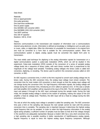
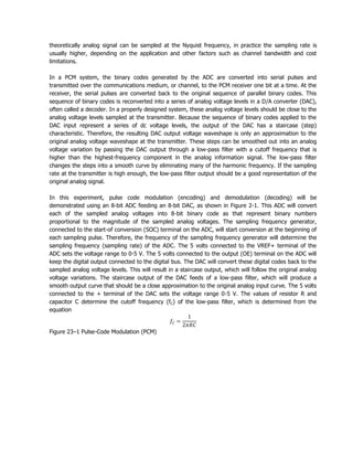
1. The experiment demonstrated pulse-code modulation (PCM) using an analog-to-digital converter (ADC) and digital-to-analog converter (DAC). 2. The DAC output had a staircase-like waveform that was smoothed into an analog signal by a low-pass filter. 3. The sampling frequency determined by the pulse generator affected the time between samples but did not change the cutoff frequency of the filter or the output frequency, which matched the input analog signal frequency.

1. NATIONAL COLLEGE OF SCIENCE & TECHNOLOGY
Amafel Bldg. Aguinaldo Highway Dasmariñas City, Cavite
EXPERIMENT 2
Digital Communication of Analog Data Using Pulse-Code Modulation (PCM)
Bani, Arviclyn C. September 20, 2011
Signal Spectra and Signal Processing/BSECE 41A1 Score:
Engr. Grace Ramones
Instructor

2. Objectives:
1. Demonstrate PCM encoding using an analog-to-digital converter (ADC).
2. Demonstrate PCM encoding using an digital-to-analog converter (DAC)
3. Demonstrate how the ADC sampling rate is related to the analog signal frequency.
4. Demonstrate the effect of low-pass filtering on the decoder (DAC) output.

3. Sample Computation
Step2
Step 6
Step 9
Step 12
Step 14
Step 16
Step 18

4. Data Sheet:
Materials
One ac signal generator
One pulse generator
One dual-trace oscilloscope
One dc power supply
One ADC0801 A/D converter (ADC)
One DAC0808 (1401) D/A converter (DAC)
Two SPDT switches
One 100 nF capacitor
Resistors: 100 Ω, 10 kΩ
Theory
Electronic communications is the transmission and reception of information over a communications
channel using electronic circuits. Information is defined as knowledge or intelligence such as audio voice
or music, video, or digital data. Often the information id unsuitable for transmission in its original form
and must be converted to a form that is suitable for the communications system. When the
communications system is digital, analog signals must be converted into digital form prior to
transmission.
The most widely used technique for digitizing is the analog information signals for transmission on a
digital communications system is pulse-code modulation (PCM), which we will be studied in this
experiment. Pulse-code modulation (PCM) consists of the conversion of a series of sampled analog
voltage levels into a sequence of binary codes, with each binary number that is proportional to the
magnitude of the voltage level sampled. Translating analog voltages into binary codes is called A/D
conversion, digitizing, or encoding. The device used to perform this conversion process called an A/D
converter, or ADC.
An ADC requires a conversion time, in which is the time required to convert each analog voltage into its
binary code. During the ADC conversion time, the analog input voltage must remain constant. The
conversion time for most modern A/D converters is short enough so that the analog input voltage will
not change during the conversion time. For high-frequency information signals, the analog voltage will
change during the conversion time, introducing an error called an aperture error. In this case a sample
and hold amplifier (S/H amplifier) will be required at the input of the ADC. The S/H amplifier accepts the
input and passes it through to the ADC input unchanged during the sample mode. During the hold
mode, the sampled analog voltage is stored at the instant of sampling, making the output of the S/H
amplifier a fixed dc voltage level. Therefore, the ADC input will be a fixed dc voltage during the ADC
conversion time.
The rate at which the analog input voltage is sampled is called the sampling rate. The ADC conversion
time puts a limit on the sampling rate because the next sample cannot be read until the previous
conversion time is complete. The sampling rate is important because it determines the highest analog
signal frequency that can be sampled. In order to retain the high-frequency information in the analog
signal acting sampled, a sufficient number of samples must be taken so that all of the voltage changes
in the waveform are adequately represented. Because a modern ADC has a very short conversion time,
a high sampling rate is possible resulting in better reproduction of high0frequency analog signals.
Nyquist frequency is equal to twice the highest analog signal frequency component. Although

5. theoretically analog signal can be sampled at the Nyquist frequency, in practice the sampling rate is
usually higher, depending on the application and other factors such as channel bandwidth and cost
limitations.
In a PCM system, the binary codes generated by the ADC are converted into serial pulses and
transmitted over the communications medium, or channel, to the PCM receiver one bit at a time. At the
receiver, the serial pulses are converted back to the original sequence of parallel binary codes. This
sequence of binary codes is reconverted into a series of analog voltage levels in a D/A converter (DAC),
often called a decoder. In a properly designed system, these analog voltage levels should be close to the
analog voltage levels sampled at the transmitter. Because the sequence of binary codes applied to the
DAC input represent a series of dc voltage levels, the output of the DAC has a staircase (step)
characteristic. Therefore, the resulting DAC output voltage waveshape is only an approximation to the
original analog voltage waveshape at the transmitter. These steps can be smoothed out into an analog
voltage variation by passing the DAC output through a low-pass filter with a cutoff frequency that is
higher than the highest-frequency component in the analog information signal. The low-pass filter
changes the steps into a smooth curve by eliminating many of the harmonic frequency. If the sampling
rate at the transmitter is high enough, the low-pass filter output should be a good representation of the
original analog signal.
In this experiment, pulse code modulation (encoding) and demodulation (decoding) will be
demonstrated using an 8-bit ADC feeding an 8-bit DAC, as shown in Figure 2-1. This ADC will convert
each of the sampled analog voltages into 8-bit binary code as that represent binary numbers
proportional to the magnitude of the sampled analog voltages. The sampling frequency generator,
connected to the start-of conversion (SOC) terminal on the ADC, will start conversion at the beginning of
each sampling pulse. Therefore, the frequency of the sampling frequency generator will determine the
sampling frequency (sampling rate) of the ADC. The 5 volts connected to the VREF+ terminal of the
ADC sets the voltage range to 0-5 V. The 5 volts connected to the output (OE) terminal on the ADC will
keep the digital output connected to the digital bus. The DAC will convert these digital codes back to the
sampled analog voltage levels. This will result in a staircase output, which will follow the original analog
voltage variations. The staircase output of the DAC feeds of a low-pass filter, which will produce a
smooth output curve that should be a close approximation to the original analog input curve. The 5 volts
connected to the + terminal of the DAC sets the voltage range 0-5 V. The values of resistor R and
capacitor C determine the cutoff frequency (fC) of the low-pass filter, which is determined from the
equation
Figure 23–1 Pulse-Code Modulation (PCM)

6. XSC2
G
T
A B C D
S1 VCC
Key = A 5V
U1
Vin D0
S2
D1
V2 D2
D3 Key = B
2 Vpk D4
10kHz
D5
0° Vref+
D6
Vref-
D7
SOC VCC
OE EOC 5V
D0
D1
D2
D3
D4
D5
D6
D7
ADC
V1 Vref+ R1
VDAC8 Output
5V -0V Vref- 100Ω
200kHz
U2
R2
10kΩ C1
100nF
In an actual PCM system, the ADC output would be transmitted to serial format over a transmission line
to the receiver and converted back to parallel format before being applied to the DAC input. In Figure
23-1, the ADC output is connected to the DAC input by the digital bus for demonstration purposes only.
PROCEDURE:
Step 1 Open circuit file FIG 23-1. Bring down the oscilloscope enlargement. Make sure that
the following settings are selected. Time base (Scale = 20 µs/Div, Xpos = 0 Y/T),
Ch A(Scale 2 V/Div, Ypos = 0, DC) Ch B (Scale = 2 V/Div, Ypos = 0, DC), Trigger
(Pos edge, Level = 0, Auto). Run the simulation to completion. (Wait for the
simulation to begin). You have plotted the analog input signal (red) and the DAC
output (blue) on the oscilloscope. Measure the time between samples (T S) on the
DAC output curve plot.
TS = 4 µs
Step 2 Calculate the sampling frequency (fS) based on the time between samples (TS)
fS = 250 kHz
Question: How did the measure sampling frequency compare with the frequency of the sampling
frequency generator?
They have a difference of 50 kHz.
How did the sampling frequency compare with the analog input frequency? Was it more than twice the
analog input frequency?
It is 20 times the analog input frequency. Yes it is more than twice the analog input frequency.
How did the sampling frequency compare with the Nyquist frequency?

7. It 6.28 times more than the sampling frequency.
Step 3 Click the arrow in the circuit window and press the A key to change Switch A to the
sampling generator output. Change the oscilloscope time base to 10 µs/Div. Run the
simulation for one oscilloscope screen display, and then pause the simulation. You are
plotting the sampling generator (red) and the DAC output (blue).
Question: What is the relationship between the sampling generator output and the DAC staircase
output?
The staircase output and the sampling generator output are both in digital form
Step 4 Change the oscilloscope time base scale to 20 µs/Div. Click the arrow in the circuit window
and press the A key to change Switch A to the analog input. Press the B key to change the
Switch B to Filter Output. Bring down the oscilloscope enlargement and run the simulation
to completion. You are plotting the analog input (red) and the low-pass filter output (blue)
on the oscilloscope
Questions: What happened to the DAC output after filtering? Is the filter output waveshape a close
representation of the analog input waveshape?
The DAC output became analog after it was being filtered. Yes.
Step 5 Calculate the cutoff frequency (fC) of the low-pass filter.
fC = 15.915 kHz
Question: How does the filter cutoff frequency compare with the analog input frequency?
They have difference of approximately 6 kHz.
Step 6 Change the filter capacitor (C) to 20 nF and calculate the new cutoff frequency (f C).
fC = 79.577 kHz
Step 7 Bring down the oscilloscope enlargement and run the simulation to completion again.
Question: How did the new filter output compare with the previous filter output? Explain.
It is almost the same.
Step 8 Change the filter capacitor (C) back to 100 nF. Change the Switch B back to the DAC output.
Change the frequency of the sampling frequency generator to 100 kHz. Bring down the
oscilloscope enlargement and run the simulation to completion. You are plotting the analog
input (red) and the DAC output (blue) on the oscilloscope screen. Measure the time
between the samples (TS) on the DAC output curve plot (blue)
TS = 9.5µs
Question: How does the time between the samples in Step 8 compare with the time between the
samples in Step 1?
It doubles.
Step 9 Calculate the new sampling frequency (f S) based on the time between the samples (TS) in
Step 8?
fS=105.26Hz
Question: How does the new sampling frequency compare with the analog input frequency?
It is 10 times the analog input frequency.
Step 10 Click the arrow in the circuit window and change the Switch B to the filter output. Bring
down the oscilloscope enlargement and run the simulation again.
Question: How does the curve plot in Step 10 compare with the curve plot in Step 4 at the higher
sampling frequency? Is the curve as smooth as in Step 4? Explain why.
Yes, they are the same. It is as smooth as in Step 4. Nothing changed. It does not affect
the filter.
Step 11 Change the frequency of the sampling frequency generator to 50 kHz and change Switch B
back to the DAC output. Bring down the oscilloscope enlargement and run the simulation to
completion. Measure the time between samples (TS) on the DAC output curve plot (blue).

8. TS = 19µs
Question: How does the time between samples in Step 11 compare with the time between the samples
in Step 8?
It doubles.
Step 12 Calculate the new sampling frequency (fS) based on the time between samples (TS) in Step
11.
fS=52.631 kHz
Question: How does the new sampling frequency compare with the analog input frequency?
It is 5 times the analog input.
Step 13 Click the arrow in the circuit window and change the Switch B to the filter output. Bring
down the oscilloscope enlargement and run the simulation to completion again.
Question: How does the curve plot in Step 13 compare with the curve plot in Step 10 at the higher
sampling frequency? Is the curve as smooth as in Step 10? Explain why.
Yes, nothing changed. The frequency of the sampling generator does not affect the filter.
Step 14 Calculate the frequency of the filter output (f) based on the period for one cycle (T).
T=10kHz
Question: How does the frequency of the filter output compare with the frequency of the analog input?
Was this expected based on the sampling frequency? Explain why.
It is the same. Yes, it is expected.
Step 15 Change the frequency of the sampling frequency generator to 15 kHz and change Switch B
back to the DAC output. Bring down the oscilloscope enlargement and run the simulation to
completion. Measure the time between samples (TS) on the DAC output curve plot (blue)
TS = 66.5µs
Question: How does the time between samples in Step 15 compare with the time between samples in
Step 11?
It is 3.5 times more than the time in Step 11.
Step 16 Calculate the new sampling frequency (fS) based on the time between samples (TS) in Step
15.
fS=15.037 kHz
Question: How does the new sampling frequency compare with the analog input frequency?
It is 5 kHz greater than the analog input frequency.
How does the new sampling frequency compare with the Nyquist frequency?
It is 6.28 times smaller than the Nyquist frequency.
Step 17 Click the arrow in the circuit window and change the Switch B to the filter output. Bring
down the oscilloscope enlargement and run the simulation to completion again.
Question: How does the curve plot in Step 17 compare with the curve plot in Step 13 at the higher
sampling frequency?
They are the same.
Step 18 Calculate the frequency of the filter output (f) based on the time period for one cycle (T).
f=10kHz
Question: How does the frequency of the filter output compare with the frequency of the analog input?
Was this expected based on the sampling frequency?
It is the same. Yes, it is expected.

9. CONCLUSION:
Therefore, I conclude that we can convert analog data to digital data through Pulse-Code
Modulation. An ADC or Analog-to –Digital Converter is use to encode PCM while DAC or Digital-to-Analog
Converter is use to decode PCM. The DAC output is looks like a staircase. The frequency is supplied by the
sampling frequency generator and is inversely proportional to the sampling time. The cutoff frequency is
generated by the capacitor and the resistor, and is not affected by the sampling frequency generator. It is
inversely proportional to the capacitance and resistance. The frequency of the output filter is the same with
the frequency of the input analog frequency, and also the waveshape of the output filter is a close
representation to the input analog signal. The sampling frequency and the DAC output are both digital while
the filter output and the input signal are both in analog.