Numerical Simulation of Flow between Two Parallel Co-Rotating Discs

International Journal of Engineering and Management Research e-ISSN: 2250-0758 | p-ISSN: 2394-6962
Volume- 9, Issue- 6 (December 2019)
www.ijemr.net https://doi.org/10.31033/ijemr.9.6.3
13 This work is licensed under Creative Commons Attribution 4.0 International License.
Numerical Simulation of Flow between Two Parallel Co-Rotating Discs
Dr. SMG. Akele1
and Prof. J.A. Akpobi2
1
Lecturer, Department of Mechanical Engineering Technology, Auchi Polytechnic, Edo State, NIGERIA
2
Lecturer, Department of Production Engineering, University of Benin, Edo State, NIGERIA
1
Corresponding Author: smg_sam2009@yahoo.com
ABSTRACT
The study of fluid flow between two rotating discs
aims to predict flow characteristics. In this paper numerical
simulation is used to investigate axisymmetric swirling flow
between two parallel co-rotating discs.
Methodology entails, firstly, inputing parameters
from CFD software are into previos study developed
dimensionless radial velocity model for flow between two
discs to obtain dimensional radial velocity of the model.
Secondly, previous study parameters are used to perform
numerical simulation on laminar and turbulent flows
between two parallel co-rotating discs. The numerical
simulation results are compared to previous study results.
Then comparative numerical simulations was carried out on
laminar and turbulent flows using CFD software.
Results obtained showed that for the this study
dimensional radial velocity and previous study
dimensionless radial velocity, radial velocity distribution
increase proportionately from the disc surface at 0m/s to
2208.00m/s and 0 to 0.0002396 respectively, at the domain
centre. And both results satisfy initial inlet and boundary
conditions with resultant parabolic profiles. In the study, it
is shown that turbulent flow radial velocity profile is
smoother than for laminar flow. The radial velocity
increases from 0 at the walls to 0.15m/s before decreasing to
- 0.2m/s at the mid-centre for laminar flow while for
turbulent flow the radial velocity intitially increases from 0
at the walls to 0.15m/s before decreasing to -0.06m/s at the
discs centre; while for laminar flow, swirl velocity decrease
from approximately 2.55m/s to 0.55m/s and for turbulent
flow the swirl velocity decrease from approximately 2.84m/s
to 1.62m/s. The turbulent flow swirl velocity profile seen to
be smoother than for laminar flow around the discs centre.
The study further showed that for fluid near the discs
surfaces radial velocity net momentum is radially towards
the outlet with flow laminar in the boundary layer region
and the velocity turbulent towards the domain centre. For
static pressure, laminar flow maximum and minimum static
pressure 2.48pa and -0.033pa respectively, while for
turbulent flow maximum and minimum static pressure were
0.00 and -0.0024pa.
The developed previous study model can therefore
be used to predict radial velocity distribution between
steady axisymmetric flow between two parallel co-rotating
discs.
Keywords-- Numerical Simulation, Radial Velocity,
Axisymmetric Flow, Corotating Discs, Swirling Flow
I. INTRODUCTION
Nikola Tesla’s 1913 turbine patent is popularly
referred to as bladeless turbine because the turbine rators
are a set of smooth closely-spaced discs connected
parallel to each other along a shaft. The bladeless turbine
operates by the fluid spiralling from the inlet at the discs
periphery inward towards the centre of the disc where it
exits through the small hole near the disc centre. In the
flow field, the fluid and discs interfaces are governed by
the principle of centripetal force, viscou sand adhesion
forces and boundary layer effects (Sengupta and Guha,
2012). In the case of a Tesla pump, the flow direction is
reversed with the fluid entering through the small holes
near the discs centre from where it spirals outwards
towards the disc peripheral. In this case centrifugal forces
come into play. Nevertheless, for both cases, as the fluid
rotates within the rotating discs, it develops viscous drag
in the boundary layer which in turns develops velocity
gradient with gains in momentum (Schosser et al., 2016;
Jose et al., 2016 ).
Tesla turbine, are not widely commercialized
because of their low efficiency unlike Tesla pumps which
are known to be commercially available since 1982 for
abrasive, viscous, shear sensitive fluids, which contain
solids. Presently, Tesla turbines find applications in
power generation, vehicle technology whike the pump is
in use as micro-polar pumps (Gupta and Kodali, 2013;
Pandey et al., 2014).
The efficiency of Tesla turbines and pumps is
known to depend on parameters such as pressure,
temperature, inlet velocity, number of discs, discs gap,
discs diameter, disc thickness, Reynolds number, angular
velocity, disc surface finish, and fluid property. Because
of its low efficiency problem their has been continued
analytically, numerically and experimentally study of
Tesla turbines (Gupta and Kodali, 2013).
With the introduction of the Tesla turbine patent,
a lot of researches and studies have been undertaken in
trying to overcome the low efficiency problem. Many, if
not all, of these studies have resulted in analytical models
that describe the flow between two discs in order to
improve on the efficiency. In past studies, the values of
parameters such as discs gap, radii ratio, number of discs
and swirl ratio, on which efficiency depends are different
for different investigator (Akpobi and Akele, 2015;
Akpobi and Akele, 2016).
1.1 Governing Equations
The PDEs governing fluid flows are the known
non-linear C-NS equations that completely describe the
flow of incompressible, Newtonian fluids. The C-NS

equations being coupled and non-linear, their solutions by
direct analytical manipulations are found to be formidable
task to overcome. (Reddy, 1993). However, simple flows
through parallel plates (e.g. Couette, Poiseuille, Couette-
Poiseuille flows) are easily solved by applying two
boundary conditions that will yield a closed-form of the
C-NS equations. This later closed-form of the governing
equations can then be solved by analytical or numerical
methods. But in the case of complex flow problems (e.g.
flows through rotating discs), these governing C-NS
equations are usually simplified into a workable closed-
form, notably by applying appropriate boundary
conditions, order of magnitude analysis, and by the use of
dimensionless parameters (Akpobi and Akele, 2016;
Sengupta and Guha, 2012).
1.2 Galerkin Integral Finite Element Method
Finite element method (FEM) is a numerical
technique for solving PDEs in which a continuous
problem described by a differential equation is put into an
equivalent variational form with approximate solution
assumed to be a linear combination of approximation
functions. One major advantage of FEM is that the
techniques can divides complex geometric domain into
sub-domains of arbitrary shape and size in order to
enhance combination of different element shapes and
computation of approximate solution. Thus, FEM
provides approximations which are better closed-form
when compared to those of other numerical methods. In
finite element analyses (FEA), the inherent coupled and
non-linearity problem of C-NS equations to flow
problems are overcome by the use of the Galerkin
weighted-residual integral approach that enables
integration of the PDEs by parts (i.e. relaxing it) to form a
‘weak’ form of the equation and (ii) choice of
approximation and interpolation functions (Reddy, 1993;
Perumal and Amon, 2011).
1.3 Computational Fluid Dynamics (CFD)
The study of fluid flow between two rotating
discs aims to predict flow characteristics. This attention
on flow between two rotating discs aroused from the need
to have comprehensive and detailed theoretical
formulations that will aid in the design of the physical
Tesla turbomachines for high efficiency. (Lopez, 1996).
II. LITERATURE REVIEW
With the introduction of the Tesla turbine patent,
a lot of researches and studies have been undertaken in
trying to overcome the low efficiency problem. Many, if
not all, of these studies have resulted in analytical models
that describe the flow between two discs in order to
improve on the efficiency. In past studies, the values of
parameters such as discs gap, radii ratio, number of discs
and swirl ratio, on which efficiency depends are different
for different investigator (Akpobi and Akele, 2015;
Akpobi and Akele, 2016).
Sengupta and Guha (2012) formulated a
mathematical model on flow for turbine configuration.
The simplified closed-form equations were solved
numerically using Lemma et al (2008) experimental data
of r1 = 13.2mm, r2= 25mm, Ω = 1000rad/s, nd = 9, Δpic =
0.113 bar for their geometry. Their results revealed that
non-dimensional tangential velocity assumed parabolic
profile between the discs, with tangential velocity
increasing from the wall (v=0) to 1.5 at the two discs
centreline, Non-dimensional radial velocity profile
between the discs was observed to be parabolic and
decreasing from 0 at the walls to -3 at the centreline. The
specified inlet tangential velocity and radial velocity wrer
10.6m/s and -11.5m/s respectively. The Fluent results
showed that tangential velocity increased with radius
from 10.6m/s at the walls (for r = 1mm) to approximately
60 m/s at the midpoint (for r = 15mm). Their result also
showed that pressure decreased from approximately 135
(at R = 0.528) to approximately 60 (at R = 1). Their
maximum theoretical efficiency obtained was 21%;
maximum power output of about 17.5 Watts at 3000rad/s
was achieved at pressure drop between inlet and exit of
Δpic = 0.113bar. Their work well agreed with Fluent 12
experimental results. Yu et al (2012) work was on
theoretical analysis and experimental study of the
pressure drop for radial inflow between co-rotating disks.
The study revealed that centrifugal and Coriolis forces are
the major factors that influenced the total pressure drop.
That is with the influence of the centrifugal and Coriolis
forces, the circumferential component of the absolute
velocity can be very high resulting in pronounced total
pressure drop in rotating cavity with radial inflow. The
total pressure drop was observed to increase with flow-
rate and Reynolds number. And at low Reynolds number,
the total pressure drop was increased by the
dimensionless mass flow-rate with the pressure increasing
first before decreasing. Pandey et al. (2014) carried out a
research study on the design and simulation analysis of 1
kW Tesla turbine in order to understand how it works.
The study revealed that high efficiencies were only obtain
at very low flow rates and the efficiencies are expected to
be under 40%. Also, it was revealed that for higher
pressure change, tangential velocities are higher with
lower flow rates. The fluid model described by Allen
(l990) was used for their CFD analysis. And fluid
parameters of dimensional system constant R* was taken
to be - 0.042 from which they judged their model to be
acceptably accurate with obtained efficiency of 77.7%.
Xing (2014) conducted direct numerical simulatiions in
order to investigate Open von Karman swirling flow
using two counterrotating coaxial discs enclosed in a
cylindrical chamber with axial extraction. In the
investigation, monotonic convergence was attained three
grids that are symmetrically refined for average pressure
at the disc outlet accompanied with small grid uncertainty
of 3.5%. Circular vortices are reported to have formed
with low discs rpm, rehardlesss of the flow rates; while
with rpm between 300 and 500, negative spiral vortex is
formed. Akpobi and Akele (2016) carried out numerical
analysis to develop two dimensional rectangular elements
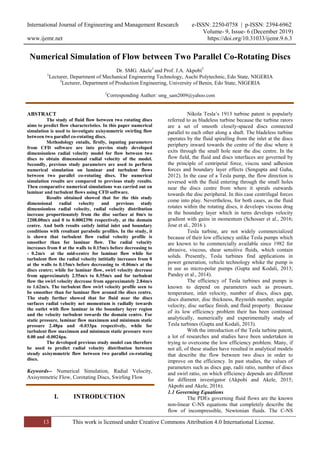
models to predict velocity components and pressure

distributions in flow between two parallel co-rotating
discs. The study revealed velocity components and
pressure solutions to converged with exact solutions as
the numbers of elements are increased with the initial
inlet and no-slip boundary conditions well satisfied.
Radial velocity was reported to increase from 0 at discs
walls to maximum of 260 at domain centreline; while
tangential velocity decreased from 0 at the walls to -1.05
at domain centreline. Radial velocity increases with radii
ration from 0 at the disc gap centreline (inlet boundary) to
maximum value of 16.23 at the disc outlet; tangential
velocity decreases from 0 at the domain inlet centreline to
-1.64 at the disc outlet and pressure increasing from 0 at
the domain centreline inlet to 32.00 at the disc outlet. The
work parametric study revealed that for different values
of Reynolds number (Re), angular velocity (ω), swirl
ratio (α), radii ratio (κ), maximum centreline velocity
(Umax) radial velocity increases with increase in all the
parameters within the disc gap. Whereas, for different
values of Reynolds number (Re), angular velocity (ω),
and radii ratio (κ) tangential velocity decreases with
increase in all the parameters within the two discs
domain; while for different values of swirl ratio (α),
angular velocity (ω), maximum velocity (Umax) and radii
ratio (κ) pressure increases from the disc inlet with
increase in all the parameters.
III. METHODOLOGY
This study pump configuration is basically a
swirling outflow configuration in which the fluid enters at
an inlet near the discs centreline (ri, z) with the outlet
along the discs periphery (ro, z). The fluid flow domain
geometry is modelled in 2D cartesian coordinates with
origin at O, the centreline between the two discs space,
Fig. 3.1.
Fig. 3.1: 2D model geometry
3.1 Boundaries Geometry
The boundaries are set as in Fig. 3.2:
Fig. 3.2: boundary conditions
(y,r)
(z,θ)
(x)
O Hole radius,r
b b
Axial in flow
Radial flow
uy
+ η- η
uy
Outlet 1
Inlet
Disc 2
Disc 1
O
Outlet 1
Inlet
Disc 2
Disc 1
Inlet
Outlet 1
x-axis
y-axis
Axial inflow

Considering the geometry of Fig 3.2, the fluid
entering at the inlet (ri , z) with initial uniform velocity (vi
= 0), comes in contact with both discs surface (solid) thus
setting up velocity gradient in the boundary layer with
no-slip boundary condition between disc-fluid interface,
and with the viscous drag in the flow domain setting up a
swirling radially outward flow in the fluid. The swirling
pathlines on a rotating disc are as shown in Fig. 3.3
(Akpobi and Akele, 2016).
Fig 3.3: Swirling pathlines of outflow
3.2 Domain Discretization
For the analysis, quadrilateral elements are used
since they are superior when compared to simple linear
triangular elements in terms of meshing and accuracy of
model meshing Perumal and Mon (2011). The domain Ω
(0 ≤ κ ≤ 1; -1 ≤ η ≤ +1) is subdivided into quadrilateral
elements mesh along the x- and y-axes respectively.
3.3 Governing Equations
For this research work, flow of fluid between the
two discs is governed by the following C-NS equations
(3.1), (3.2), (3.3) and (3.4) in Cartesian coordinates
(Akpobi and Akele, 2015; Akpobi and Akele, 2016):
Continuity equation:
     
0
yx z
uu u
t x y z
   
   
   
(3.1)
x-momentum equation:
2 2 2
2 2 2
1
3
yx x x x x x xX z
x y z x
uu u u u u u uu up
u u u g
t x y z x x y z x x y z
   
            
               
               
(3.2)
y-momentum equation:
2 2 2
2 2 2
1
3
y y y y y y y yx z
x y z y
u u u u u u u uu up
u u u g
t x y z y y x y zx y z
   
             
                              
(3.3)
z-momentum equation:
2 2 2
2 2 2
1
3
yxz z z z z z z z
x y z z
uuu u u u u u u up
u u u g
t x y z z z x y zx y z
   
             
               
               
(3.4)
3.4 Relevant Assumptions
In order to simplify the non-linear C-NS
equations (3.1) through (3.4) to workable level, the
following assumptions are made (Akpobi and Akele,
2016):
(i) flow is analysed in 2D,
(ii) flow is in the radial direction and
symmetrical over z-coordinate with very
large discs radius and small gap,
incompressible, steady, and viscous
flow,
(iii) flow in z-axis direction assumed
insignificantly negligible,
(iv) body forces (gravitational and inertia ) are
negligible,
(v) no-slip condition exists at discs faces,
ri
ro
z
θ
r
v
w
u
Spiralling velocity pathline

(vi) both discs angular velocities are constant
and equal.
3.5 Boundary Conditions
The following boundary conditions are specified
at the domain inlet, outlet and boundaries:
At the discs hole inlet:
( , ) 0.2 /
( , 0) 0
i i
i
axial
v x y m s
radial
u x
  

(3.5)
Static pressure at outlet:
( , ) 0op y x  (3.6)
At the two discs-fluid interfaces:
( , ) 0; ( , ) 0
( , ) 0; ( , ) 0,
u y x u y x
v y x v y x
   
   
(3.7)
At the discs walls:
1 2( , ) ( , ) 70o oD y x D y x rpm     (3.8)
3.6 Method of Solution
The method of solution used for simulation is
ANSYS 16.2 CFD software. ANSYS Fluid Flow (Fluent)
analysis system was used to draw the model geometry,
generate the model quadrilateral meshes and then using
the Fluent Solver to obtain the solutions. The 2D analysis
was set up on 2D space, pressure-based, absolute velocity
formulation, steady and axisymmetric swirling flow.
In this study, parameters from the CFD software
are input into Akpobi and Akele (2016) developed radial
velocity (dimensionless) model for flow between two
discs to obtain dimensional radial velocity of the model.
These input parameters, initial inlet and boundary
conditions and disc geometry are shown in Table 1, Table
2 and Table 3 respectively.
Table 3.1: water properties
Water properties
Density 1000kg/m3
Viscosity 0.00089N.s/m2
Temperature 300K
Pressure 1atm
Specific heat capacity 1006.43J/kg.K
Thermal conductivity 0.0242W/m.K
Molecular weight 28.966kg/kgmol
Table 3.2: initial and boundary conditions
Initial and Boundary conditions
Axial Inlet velocity 0.20 m/s
Radial Inlet velocity 0 m/s
Outlet pressure 0 pa
Discs angular velocity 75rpm (7.85rad/s)
Swirl velocity 0rpm
Table 3.3: discs model geometry
Discs model geometry
Number of nodes 2339
Disc diameter 100cm
Inlet hole diameter 4cm
Discs thickness 0cm
Discs gap 10cm
IV. RESULTS AND DISCUSSION The following table and figures show the results
obtained.

Table 4.1: values of dimensionless (Akpobi and Akele, 2016) and dimensional (present study)
(κ, η = 0) Akpobi and Akele (2015)
(dimensionless)
This study
(m/s)
0 0.0000000 0.00
0.125 0.0000561 517.46
0.250 0.0001048 965.92
0.333 0.0001460 1345.00
0.375 0.0001797 1656.00
0.500 0.0002059 1897.00
0.625 0.0002247 2070.00
0.667 0.0002359 2173.00
0.750 0.0002396 2208.00
Fig. 4.1: dimensionless radial velocity
Fig. 4.2: dimensional radial velocity
1 0.8 0.6 0.4 0.2 0 0.2 0.4 0.6 0.8 1
0
2.396 10
5

4.792 10
5

7.188 10
5

9.584 10
5

1.198 10
4

1.4376 10
4

1.6772 10
4

1.9168 10
4

2.1564 10
4

2.396 10
4

Radial velocity against discs gap
discs-gap
radialvelocity(dimensionless)
u8 ( )

Fig. 4.3: dimensionless radial velocity distribution
0
0.00005
0.0001
0.00015
0.0002
0.00025
0.0003
0 0.125 0.25 0.333 0.375 0.5 0.625 0.667 0.75
radialvelocity
(dimensionless)
Radial velocity vs half disc-gap
0
500
1000
1500
2000
2500
0 0.125 0.25 0.333 0.375 0.5 0.625 0.667 0.75
radialvelocity,m/s
Radial velocity vs half disc-gap

1 0.8 0.6 0.4 0.2 0 0.2 0.4 0.6 0.8 1
0
300
600
900
1.2 10
3

1.5 10
3

1.8 10
3

2.1 10
3

2.4 10
3

2.7 10
3

3 10
3

Radial velocity against disc gap
disc gap (m)
Radialvelecity(m/s)
uA ( )( )

Fig. 4.4: dimensional radial velocity distribution
Fig 4.5: simulations mesh
Fig 4.6: laminar radial velocity distribution Fig 4.7: turbulent radial velocity distribution

Fig 4.8: laminar flow swirl velocity Fig 4.9: turbulent flow swirl velocity
Fig 4.10: laminar flow contour of radial velocity Fig 4.11: turbulent flow contour of radial velocity
Fig 4.12: laminar flow velocity vector magnified Fig 4.13: turbulent flow velocity vector magnified
Fig 4.14: Laminar flow contour of static prssure Fig 4.15: turbulent flow contour of static prssure

Table 4 shows the result obtained for
dimensionless Akpobi and Akele (2016) and dimensional
present study. The difference in values can be attributed
to analysis inherent analytical errors, numerical
computations errors, domain discretization errors and
solution approximation errors of Galerkin integral finite
element method used.
Fig. 4.1 and Fig. 4.2 are the dimensionless
(Akpobi and Akele, 2016) and dimensional (present
study) plots of radial velocity against half the disc gap
(from one surface to the centre). Both distributions
increase proportionately from the disc surface at 0 to the
centre 0.0002396 (dimensionless) and 2208.00m/s
respectively. While Fig. 4.3 and Fig. 4.4 are the
dimensionless and dimensional plots of radial velocity
over the flow domain (between the two discs surfaces)
with minimum and maximum velocities of 0 and
0.0002396 (dimensionless) and 0 and 2208.00m/s
respectively. And both curves satisfy initial inlet and
boundary conditions with parabolic profile.
In Fig.4.6 and Fig 4.7, it is shown that turbulent
flow radial velocity profile is smoother than for laminar
flow. The radial velocity increases from 0 at the walls to
0.15m/s before decreasing to -0.2m/s at the mid-centre
for laminar flow while for turbulent flow the radial
velocity intitially increases from 0 at the walls to 0.15m/s
before decreasing to -0.06m/s at the discs centre. Fig.4.8
and Fig 4.9 show laminar and turbulent flow swirl
velocity distribution between the two discs. For laminar
flow, Fig 4.8 shows that the swirl velocity decrease from
approximately 2.55m/s to 0.55m/s; while for turbulent
flow, Fig 4.9, the swirl velocity decrease from
approximately 2.84m/s to 1.62m/s. The turbulent flow
swirl velocity profile seen to be smoother than for
laminar flow around the discs centre. In Fig.4.10 and Fig
4.11, it is shown that turbulent flow radial velocity profile
is smoother than for laminar flow. The radial velocity
increases from 0 at the walls to 0.15m/s before decreasing
to -0.2m/s at the mid-centre for laminar flow while for
turbulent flow the radial velocity intitially increases from
0 at the walls to 0.15m/s before decreasing to -0.06m/s at
the discs centre. Fig. 4.12 and Fig. 4.13 show that for
fluid near the discs surfaces radial velocity net
momentum is radially towards the outlet. Fig. 4.12 show
flow to be laminar in the boundary layer region while in
Fig. 4 13 the velocity is shown be in turbulent, especially
towards the domain centre.
In Fig. 4.14, laminar flow, maximum and
minimum static pressure contour are shown respectively
as 2.48pa and -0.033pa while for turbulent flow, Fig.
4.15, maximum and minimum static pressure contour are
respectively 0.00 and -0.0024pa. For turbulent flow,
stataic pressure is higher close to the outlet than for
laminar flow.
V. CONCLUSIONS
In this study, firstly, parameters from CFD
software are input into Akpobi and Akele (2016)
developed radial velocity (dimensionless) model for flow
between two discs to obtain dimensional radial velocity
of the model. Secondly, previous study parameters are
used to perform numerical simulation on laminar and
turbulent flows between two parallel co-rotating discs.
The numerical simulation results are compared to
previous study results. Comparative numerical
simulations was carried out on laminar and turbulent
flows using CFD software.
The results obtained show negligible difference
in result obtained for this study simulation and previous
study reslt. And the dimensionless previous study and this
study dimensional radial velocity distributions both
increase, proportionately, from the discs surfaces to the
fluid flow domain centre while satisfying the initial inlet
and boundary conditions.
The developed previous model can therefore be
used to predict radial velocity distribution between steady
axisymmetric flow between two parallel co-rotating discs.
RECOMMENDATIONS
For for study, a 3-dimension simulation be
investigated. This ill allow for consideration of tangential
velocity prediction along side radial velocity.
REFERENCES
[1] Akpobi, J. A. & Akele, SMG. (2015). Development of
finite element models for predicting velocities and
pressure distribution for viscous fluid flow between two
parallel co-rotating discs. International Journal of
Engineering and Management Research, 5(6), 724-742.
[2] Akpobi, J. A. & Akele, SMG. (2016). Development of
2D models for velocities and pressure distribution in
viscous flow between two parallel co-rotating discs.
Journal of the Nigerian Association of Mathematical
Physics, 2, 233–290.
[3] Gupta, H. & Kodali, S. P. (2013). Design and
operation of Tesla turbo-machine – A state of the art
view. International Journal of Advanced Transport
Phenomena, 2(1), 7-14.
[4] Jose, R., Jose, A., Benny, A., salus, A., & Benny, B.
(2016). A theoretical study on surface finish, spacing
between discs and performance of Tesla turbine.
International Advanced Research Journal in Science,
Engineering and technology, 3(3), 235-240.
[5] Lopez, J. M. (1996). Flow between a stationary and a
rotating disc shrouded by a co-rotating cylinder. Physics
of Fluid, 8(10), 2605-2613.
[6] Pandey, R. J., Pudasaini, S., Dhakal, S., Uprety, R. B.,
& Neopane, H. P. (2014). Design and computational
analysis of 1kW Tesla Turbine. International Journal of
Scientific and Research Publications, 4(11), 141-145.
[7] Perumal, L. & Mon, D. T. T. (2011 ). Finite elements
for engineering analysis: A brief review. International

Conference on Modeling, Simulation and Control
IPCSIT, 10, Singapore: IACSIT Press. Available at:
www.ipcsit.com/vol10/12-ICMSC2011S034.
[8] Reddy, J. N. (1993). An introduction to the finite
element method. (2nd
ed.). New York: McGraw-Hill, Inc.
[9] Schosser, C., Lecheler, S., & Pfitzner, M. (2016).
Analytical and numerical solutions of the rotor flow in
Tesla turbine. Periodica Polytechnica Mechanical
Engineering, 61(1), 12-22.
[10] Sengupta, S. & Guha, A. (2012). A theory of Tesla
disc turbines. Journal of Power and Energy, 266(5), 650-
663.
[11] Soong, C. (1996). Prandtl number effects on mixed
convection between rotating coaxial discs. International
Journal of Rotating Machinery, 2(3), 161-166.
[12] Xing, T. (2014). Direct numerical simulation of open
von karman swirling flow. Journal of Hydrodynamics,
26(2), 165-177.
[13] Yu, X., Lu, H. Y., Sun, J. N., Luo, X., & Xu, G. Q.
(2012). Study of the pressure drop for radial inflow
between co-rotating disks. 28th
International Congress of
The Aeronautical Sciences. Available at:
https://academictree.org/sociology/publications.php?pid=
182803.

Numerical Simulation of Flow between Two Parallel Co-Rotating Discs

Recommended

Recommended

More Related Content

What's hot

What's hot (19)

Similar to Numerical Simulation of Flow between Two Parallel Co-Rotating Discs

Similar to Numerical Simulation of Flow between Two Parallel Co-Rotating Discs (20)

More from Dr. Amarjeet Singh

More from Dr. Amarjeet Singh (20)

Recently uploaded

Recently uploaded (20)

Numerical Simulation of Flow between Two Parallel Co-Rotating Discs