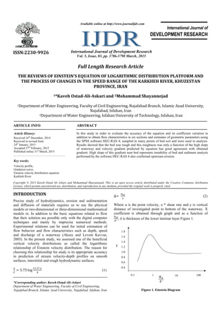
SlideShare a Scribd company logo
1 of 5
Download to read offline
Full Length Research Article
THE REVIEWS OF EINSTEIN'S EQUATION OF LOGARITHMIC DISTRIBUTION PLATFORM AND
THE PROCESS OF CHANGES IN THE SPEED RANGE OF THE KARKHEH RIVER, KHUZESTAN
PROVINCE, IRAN
1*Kaveh Ostad-Ali-Askari and 2Mohammad Shayannejad
1Department of Water Engineering, Faculty of Civil Engineering, Najafabad Branch, Islamic Azad University,
Najafabad, Isfahan, Iran
2Department of Water Engineering, Isfahan University of Technology, Isfahan, Iran
ARTICLE INFO ABSTRACT
In this study in order to evaluate the accuracy of the equation and its coefficient variation in
addition to obtain flow characteristics in six sections and estimates of geometric parameters using
the SPSS software HEC-RAS 4, sampled in many points of bed soil and were used in analysis.
Results showed that the bed was rough and this roughness was only a function of the high slope
of waterway and velocity gradient predicted by equation has good agreement with obtained
gradient. High slope of this gradient near bed represents instability of bed and sediment analysis
performed by the software HEC-RAS 4 also confirmed upstream erosion.
Copyright © 2015 Kaveh Ostad Ali Askari and Mohammad Shayannejad. This is an open access article distributed under the Creative Commons Attribution
License, which permits unrestricted use, distribution, and reproduction in any medium, provided the original work is properly cited.
INTRODUCTION
Precise study of hydrodynamics, erosion and sedimentation
and diffusion of materials requires us to use the physical
models or two-dimensional or three-dimensional mathematical
models in. In addition to the basic equations related to flow
that their solution are possible only with the digital computer
techniques and manly by imprecise numerical methods.
Experimental relations can be used for initial estimation of
flow behavior and flow characteristics such as depth, speed
and discharge of a waterway (Aksoy and Levent Kavvas,
2005). In the present study, we assessed one of the beneficial
vertical velocity distributions as called the logarithmic
relationship of Einstein velocity distribution. The reason for
choosing this relationship for study is its appropriate accuracy
in prediction of stream velocity-depth profiles on smooth
surfaces, interstitial and rough hydrodynamic surfaces.
= 5.75 log
. 	
∆
(1)
*Corresponding author: Kaveh Ostad-Ali-Askari
Department of Water Engineering, Faculty of Civil Engineering,
Najafabad Branch, Islamic Azad University, Najafabad, Isfahan, Iran
∆=	 (2)
Where u is the point velocity, u * shear rate and y is vertical
distance of investigated point to bottom of the waterway. X
coefficient is obtained through graph and as a function of
, δ is thickness of the lower laminar layer Figure 1.
Figure 1. Einstein Diagram
ISSN:2230-9926 International Journal of Development Research
Vol. 5, Issue, 03, pp. 3786-3790 March, 2015
International Journal of
DEVELOPMENT RESEARCH
Article History:
Received 16th
December, 2014
Received in revised form
24th
January, 2015
Accepted 27th
February, 2015
Published online 31st
March, 2015
Key words:
Velocity profile,
Gradation curve,
Einstein velocity distribution equation
Karkheh River
Available online at http://www.journalijdr.com
1.8
1.6
1.4
1.2
1/0
0.8
0.6
0.4
0.1 1 10 100
=	
. 	
∗
(3)
X factor depending on the roughness of the bottom varies
between 0.69 to 1.63 and for the hydrodynamic rough surfaces
is equal to 1. Thus can be said Δ value is equal to D65for the
rough surfaces. The aim of this study was evaluation of the
equation accuracy and estimation of Δ coefficient in velocity
distribution equation and whether the correction factor Δ (X)
change in the range of studies result or not. This velocity
distributions equation can be used easily by finding Δ changes
in period of study (Einstein and Harder, 1954).
MATERIALS AND METHODS
The theoretical equations of velocity distribution
In general, we faced to flow in waterways that its boundary
layer is turbulent. Turbulent boundary layer is more complex
than laminar boundary layer. In laminar lower layer, the
velocity distribution is based on Newton's law of viscosity that
is related to shear stress and viscosity. Assuming that the shear
is almost constant and equal to stress on wall (τ), we have:
= (4)
Where μ is viscosity, is velocity gradient and u is
velocity at the point with y distance from the wall (boundary).
After integrating the last equation under boundary condition
(u=0, y=0) the following result is obtained:
= (5)
In attention to ( 	=	 ) and ( ) we have:
∗
= ∗
(6)
Out of the laminar lower layer, flow is turbulent, so there is a
different form of the velocity distribution. In this layer, in
addition to the viscosity force of the layer due to the mixing of
the fluid particles, small whirlpools and cross currents, other
shear stress that is called apparent shear stresses or Reynolds
stresses arise. Thus, according to the theory of Prandtlmixing
length and Carmen similarity theory for turbulence can be
written as:
= 	
(7)
Where: τ is shear stress at the point where its distance from the
y plate and velocity gradientis ( ) at that point. Based on
measurements, shear stress in the proximity of plate can be
equal to shear stress on the plate ( =	 ), thus:
= 	 	
(8)
And because ( ∗ =	 ), and approximately k = 0.4, we have:
= 2.5	
∗
(9)
After integration of the recent equation under the condition u =
0 at y = y ', the result would be:
∗
= 2.5 ln ′ = 5.75 log ′ (10)
In the last equation y ' is the integration constant and u is
velocity at the point where its distance from solid boundary is
y. Constant value of y 'must be determined by empirical data,
that its value is different depending on the boundary is smooth
or rough. The last equation is known as wall logarithmic law
and when credit that = 0.2.,In < 0.2, firstly the shear stress
is nearly constant and equal to the boundary shear stress( ),
secondly, the effect of pressure gradient is negligible. This
region (0< <0.2) is often called internal region. Out of this
region (0≤ ≤0.2) is called external region. Internal region
includes a laminar lower layer and velocity distribution is
logarithmic in this region. The thickness of the inner region in
each place is approximately 20% of the thickness of boundary
layer (Wu and Moin, 2009 and Bhattacharyya et al., 2011).
Nikuradze for smooth and rough surfaces (pipe and channel)
after determining the integral constant (y ') in the above
equation based on the experimental results presented the
following equation for the velocity distribution in the internal
area:
∗
= 5.75 log
∗
+ 5.5 for smooth border (11)
∗
= 5.75 log
∗
+ 8.5	for rough border (12)
The velocity distribution equation is similar to above equation
for the boundary that is interstitial the smooth and rough
(interstitial boundary), except that constant value of
relationship changes between 8.6 to 5.8.The results observed
in the outer region of the boundary layer (0.2≤ ≤1) in
waterways show that we can used reduction velocity law for
the velocity distribution in this region. According to the
reduction velocity law, velocity distribution equation for
smooth and rough surfaces is:
∗
= 575 log + (13)
Where Umax is velocity at the outer edge of the boundary layer
and δ is boundary layer thickness and A is numeric value that
must be determined by experiment. Qligan obtained following
relationships for u velocity:
∗
= 575 log
∗
+ 	for smooth channel (14)
∗
= 575 log + 	for rough channel (15)
In recent equations, AS and AR are constant values that their
values were determined 3.25 and 6.25, respectively, by Qligan.
3787 Kaveh Ostad-Ali-Askari and Mohammad Shayannejad, The reviews of Einstein's equation of logarithmic distribution platform and the process
of changes in the speed range of the Karkheh river, Khuzestan province, Iran
Experimental results showed that AS and AR values are not
constant value and depend on Froude number. The results of
this analysis demonstrate for Froude numbers less than 4,
ASvalue remains constant, so the above equation can be used
in most practical program, with assuming that AS and ARare
constant. Above equations cannot be used to waterways that
their bottom is interstitialhydro-dynamically. Einstein and
Barbarossa based on Nikuradze study, presented the following
equation to determine the speed of the channels with smooth,
Interstitial and coarse surface.
∗
= 5.75 log
. 	
∆
(16)
∆	=	 (17)
In the above equation, X is correction factor that is the
function of D65 / δ 'and its value must be determined from the
curve. Therefore, the above equation along with the curves can
be used to any surface (Denicol et al., 2010 and Huai et al.,
2009).
Studies range from the foot bridge to Shush, Khuzestan
province, Iran
Study area was selected ranges of Karkheh River with a length
of 41 km from the foot bridge to Shush, Khuzestan province,
Iran. 6 sections in interval, 2 sections at the end of interval and
4 sections in the intermediate interval were selected. Sections
were recorded by echo sounder and total station camera
RTS538 over 3 weeks. Taken sections were introduced to
HEC-RAS4 software to obtain fastly geometric parameters in
each section in different surface water balance Interval scheme
shown in Figure 2.
Figure 2. In the fields of bridge-foot interval of Shush, Khuzestan
province, Iran
After marking sections, flow characteristics were obtainedin
studies section during a few weeks. Obtained characteristics
including the measurement of the mean velocity by dividing
each section to 5 subsection and estimating the average speed
of each subsection by three-point method using the Molinet,
measurement the slope of the water surface, estimate the
geometric parameters such as cross section, wetted area and
the water level width for each section by software geometric
characteristics of taken sections are displayed in Figure 3.
Figure 3. The geometric characteristics of the harvested sections0 km to 27.34 km
Bridge
Shoosh
3788 International Journal of Development Research, Vol. 05, Issue, 03, pp. 3786-3790 March, 2015
After the riverbed soil sampling in studies area and applying
grading test, we observed that type of riverbed was loamy
coarse sand and size of riverbed particles decreased from
upstream to downstream. The data collected is shown in Table
1.
Conclusion
The surface of waterway in the entire ranges of study is rough
hydrodynamically and the roughness is independent from
bottom particle size. The main factor of rough floor
hydrodynamically, is steep slope especially in the upstream
bed. So can be said that, correction coefficient X is equal to
1and Δ is equal to D65.
After speed deep profile drawing in each section using
collected data and comparison with the velocity predicted
profiles by Einstein's equation can be realized high accuracy of
this equation for rough surfaces. Velocity gradient predicted
by the equation has good agreement with obtained gradient
from the study sections, particularly near the bed and high
slope of gradient to the vertical line represents the high speed
and high turbulence near the ground and consequently
instability of bed and this prediction with results of the
sediment analysis has confirmed the preferred Yung method in
HEC-RAS software (version 4). Prediction of 5-year
longitudinal bed profile changes by the Yung pattern was
shown in Figure 4. As seen in the upstream interval the
dominant phenomenon was erosion and in downstream
Table 1. Section 1- 0 km
Date A P V Rh Sf U* N d-
D65
2005/04/21 416.38 189.28 0.7 2.19981 0.000125 0.051927 1E-06 0.000225 0.004
2005/04/22 573.26 207.21 0.91 2.76657 0.000157 0.0652629 1E-06 0.000169 0.004
2005/04/23 540.5 206.31 0.86 2.61984 0.000151 0.0622834 1E-06 0.000177 0.004
2005/04/24 506.29 205.36 0.81 2.46538 0.000145 0.0592068 1E-06 0.000187 0.004
2005/04/25 469.85 204.35 0.77 2.29924 0.000141 0.056383 1E-06 0.000196 0.004
Table 2. Section 2- 7.8 km
Date A P V Rh Sf U* N d-
D65
2005/04/21 181.99 95.89 1.57 1.898 0.000766 0.1193981 1E-06 9.76E-0.5 0.004
2005/04/28 179.85 92.8 1.56 1.938 0.000737 0.118348 1E-06 9.85E-0.5 0.004
2005/04/29 146.02 61.6 1.36 2.37 0.000424 0.0992761 1E-06 0.000117 0.004
2005/04/30 154.79 75.88 1.38 2.04 0.000539 0.103836 1E-06 0.000112 0.004
2005/04/31 138.77 48.47 1.33 2.863 0.000315 0.09404 1E-06 0.000124 0.004
Table 3. Section 3- 20.09 km
Date A P V Rh Sf U* N d-
D65
2005/05/01 96.24 60.31 2.9 1.596 0.00328 0.226551 1E-06 5.15 E-0.5 0.0035
2005/05/02 64.18 59.17 2.59 1.085 0.004377 0.2157661 1E-06 5.4 E-0.5 0.0035
2005/05/03 90.05 59.89 2.83 1.504 0.003549 0.2288715 1E-06 5.1 E-0.5 0.0035
2005/05/04 205.6 60.09 2 3.422 0.003409 0.3381971 1E-06 3.45 E-0.5 0.0035
2005/05/05 36.37 54.87 2.39 0.664 0.007203 0.2165525 1E-06 5.38 E-0.5 0.0035
Table 4. Section 4- 27.34 km
Date A P V Rh Sf U* N d-
D65
2005/05/09 164.45 145.18 1.7 1.133 0.00148 0.1282125 1E-06 9.09E-0.5 0.003
2005/05/10 161.33 142.21 1.704 1.134 0.00149 0.1287475 1E-06 9.06 E-0.5 0.003
2005/05/11 164.03 144.88 1.707 1.132 0.001479 0.1281408 1E-06 9.01 E-0.5 0.003
2005/05/12 143.97 113.25 1.61 1.271 0.001487 0.1361502 1E-06 8.56 E-0.5 0.003
2005/05/13 146.47 113.33 1.625 1.292 0.001481 0.1370015 1E-06 8.51 E-0.5 0.003
Table 5. Section 5- 34.73 km
Date A P V Rh Sf U* N d-
D65
2005/05/14 170.15 153.01 1.38 1.112 0.001022 0.1055668 1E-06 0.00011 0.002
2005/05/15 191.13 158.33 1.39 1.207 0.000962 0.1067127 1E-06 0.000109 0.002
2005/05/16 179.14 155.33 1.38 1.153 0.00099 0.1058181 1E-06 0.00011 0.002
2005/05/17 243.07 208.68 1.403 1.165 0.000917 0.1023523 1E-06 0.000114 0.002
2005/05/18 174.06 154 1.384 1.13 0.001 0.1052774 1E-06 0.000111 0.002
Table 6. Section 6- 40.83 km
Date A P V Rh Sf U* N d-
D65
2005/05/21 112.3 98.9 1.344 1.135 0.000818 0.0954365 1E-06 0.000122 0.002
2005/05/22 131.67 127.54 1.39 1.032 0.000816 0.090889 1E-06 0.000128 0.002
2005/05/23 122.33 115.84 1.37 1.056 0.000817 0.0919802 1E-06 0.000127 0.002
2005/05/24 113.4 101.47 1.35 1.118 0.000818 0.0946804 1E-06 0.000123 0.002
2005/05/25 93.07 78.96 1.16 1.179 0.000691 0.0893689 1E-06 0.00013 0.002
3789 Kaveh Ostad-Ali-Askari and Mohammad Shayannejad, The reviews of Einstein's equation of logarithmic distribution platform and the process
of changes in the speed range of the Karkheh river, Khuzestan province, Iran
interval was not observed any changes (The model outputs is
increased for better understanding ).
REFERENCES
Aksoy, H. and Levent Kavvas, M. 2005.“A review of hillslope
and watershed scale erosion and sediment transport
models”. CATENA, Vol. 64, No. 2-3, pp. 247–271.
doi:10.1016/j.catena.2005.08.008.
Bhattacharyya, K., Mukhopadhyay, S. and Layek, G. C. 2011.
“Slip effects on boundary layer stagnation-point flow and
heat transfer towards a shrinking sheet”. International
Journal of Heat and Mass Transfer, Vol. 5, No. 1-3, pp.
308–313. doi:10.1016/j.ijheatmasstransfer.2010.09.041.
Denicol, G.S., Koide, T. and Rischke, D. H. 2010.
“Dissipative relativistic fluid dynamics: a new way to
derive the equations of motion from kinetic theory”. Phys
Rev Lett, Vol. 105, No. 16, pp.162501.DOI:
http://dx.doi.org/10.1103.
Einstein, H. A. and Harder, J. A. 1954.”Velocity distribution
and the boundary layer at channel bends”. Eos,
Transactions American Geophysical Union, Vol. 35, No. 1,
pp.114–120. DOI: 10.1029/TR035i001p00114.
Huai, W. X., Han, J., Zeng, Y. H., An, X. and Qian, Z. D.
2009. “Velocity distribution of flow with submerged
flexible vegetations based on mixing-length approach”.
Applied Mathematics and Mechanics, Vol. 30, No. 3, pp.
343-351. DOI: 10.1007/s10483-009-0308-1.
Wu, X. and Moin, P. 2009.“Direct numerical simulation of
turbulence in a nominally zero-pressure-gradient flat-plate
boundary layer”. Journal of Fluid Mechanics, Vol. 630,
pp. 5- 41. DOI: http://dx.doi.org/10.1017/
S0022112009006624.
*******
3790 International Journal of Development Research, Vol. 05, Issue, 03, pp. 3786-3790 March, 2015

More Related Content

What's hot

Comparison of flow analysis of a sudden and gradual change of pipe diameter u...
Comparison of flow analysis of a sudden and gradual change of pipe diameter u...Comparison of flow analysis of a sudden and gradual change of pipe diameter u...
Comparison of flow analysis of a sudden and gradual change of pipe diameter u...eSAT Journals
 
Comparison of flow analysis of a sudden and gradual change
Comparison of flow analysis of a sudden and gradual changeComparison of flow analysis of a sudden and gradual change
Comparison of flow analysis of a sudden and gradual changeeSAT Publishing House
 
Simulation of segregated flow over the 2 d cylinder using star ccm+
Simulation of segregated flow over the 2 d cylinder using star ccm+Simulation of segregated flow over the 2 d cylinder using star ccm+
Simulation of segregated flow over the 2 d cylinder using star ccm+Burak Turhan
 
Effect of Geometry on Variation of Heat Flux and Drag for Launch Vehicle -- Z...
Effect of Geometry on Variation of Heat Flux and Drag for Launch Vehicle -- Z...Effect of Geometry on Variation of Heat Flux and Drag for Launch Vehicle -- Z...
Effect of Geometry on Variation of Heat Flux and Drag for Launch Vehicle -- Z...Abhishek Jain
 
Laminar boundary layer
Laminar boundary layerLaminar boundary layer
Laminar boundary layerFarzad Hossain
 
Comparision of flow analysis through a different geometry of flowmeters using...
Comparision of flow analysis through a different geometry of flowmeters using...Comparision of flow analysis through a different geometry of flowmeters using...
Comparision of flow analysis through a different geometry of flowmeters using...eSAT Publishing House
 
Analysis of vortex formation around a circular cylinder at low Reynolds number
Analysis of vortex formation around a circular cylinder at low Reynolds numberAnalysis of vortex formation around a circular cylinder at low Reynolds number
Analysis of vortex formation around a circular cylinder at low Reynolds numbereditorijrei
 
Properties of Fluids, Fluid Static, Buoyancy and Dimensional Analysis
Properties of Fluids, Fluid Static, Buoyancy and Dimensional AnalysisProperties of Fluids, Fluid Static, Buoyancy and Dimensional Analysis
Properties of Fluids, Fluid Static, Buoyancy and Dimensional AnalysisSatish Taji
 
Application of DRP scheme solving for rotating disk-driven cavity
Application of DRP scheme solving for rotating disk-driven cavityApplication of DRP scheme solving for rotating disk-driven cavity
Application of DRP scheme solving for rotating disk-driven cavityijceronline
 
Fluid dynamics 1
Fluid dynamics 1Fluid dynamics 1
Fluid dynamics 1guest7b51c7
 
Numerical Analysis of MHD Flow of Fluid with One Porous Bounding Wall
Numerical Analysis of MHD Flow of Fluid with One Porous Bounding WallNumerical Analysis of MHD Flow of Fluid with One Porous Bounding Wall
Numerical Analysis of MHD Flow of Fluid with One Porous Bounding WallIRJET Journal
 
fluid mechanics pt1
fluid mechanics pt1fluid mechanics pt1
fluid mechanics pt1Shanu Jp
 
Prediction of aerodynamic characteristics for slender bluff bodies with nose ...
Prediction of aerodynamic characteristics for slender bluff bodies with nose ...Prediction of aerodynamic characteristics for slender bluff bodies with nose ...
Prediction of aerodynamic characteristics for slender bluff bodies with nose ...vasishta bhargava
 

What's hot (19)

Comparison of flow analysis of a sudden and gradual change of pipe diameter u...
Comparison of flow analysis of a sudden and gradual change of pipe diameter u...Comparison of flow analysis of a sudden and gradual change of pipe diameter u...
Comparison of flow analysis of a sudden and gradual change of pipe diameter u...
 
Comparison of flow analysis of a sudden and gradual change
Comparison of flow analysis of a sudden and gradual changeComparison of flow analysis of a sudden and gradual change
Comparison of flow analysis of a sudden and gradual change
 
Simulation of segregated flow over the 2 d cylinder using star ccm+
Simulation of segregated flow over the 2 d cylinder using star ccm+Simulation of segregated flow over the 2 d cylinder using star ccm+
Simulation of segregated flow over the 2 d cylinder using star ccm+
 
Effect of Geometry on Variation of Heat Flux and Drag for Launch Vehicle -- Z...
Effect of Geometry on Variation of Heat Flux and Drag for Launch Vehicle -- Z...Effect of Geometry on Variation of Heat Flux and Drag for Launch Vehicle -- Z...
Effect of Geometry on Variation of Heat Flux and Drag for Launch Vehicle -- Z...
 
Laminar boundary layer
Laminar boundary layerLaminar boundary layer
Laminar boundary layer
 
Comparision of flow analysis through a different geometry of flowmeters using...
Comparision of flow analysis through a different geometry of flowmeters using...Comparision of flow analysis through a different geometry of flowmeters using...
Comparision of flow analysis through a different geometry of flowmeters using...
 
D0421020028
D0421020028D0421020028
D0421020028
 
Analysis of vortex formation around a circular cylinder at low Reynolds number
Analysis of vortex formation around a circular cylinder at low Reynolds numberAnalysis of vortex formation around a circular cylinder at low Reynolds number
Analysis of vortex formation around a circular cylinder at low Reynolds number
 
Fluid flow
Fluid flowFluid flow
Fluid flow
 
Chapter 4. diffrential
Chapter 4. diffrentialChapter 4. diffrential
Chapter 4. diffrential
 
Fluid Mechanics - Fluid Properties
Fluid Mechanics - Fluid PropertiesFluid Mechanics - Fluid Properties
Fluid Mechanics - Fluid Properties
 
Properties of Fluids, Fluid Static, Buoyancy and Dimensional Analysis
Properties of Fluids, Fluid Static, Buoyancy and Dimensional AnalysisProperties of Fluids, Fluid Static, Buoyancy and Dimensional Analysis
Properties of Fluids, Fluid Static, Buoyancy and Dimensional Analysis
 
Application of DRP scheme solving for rotating disk-driven cavity
Application of DRP scheme solving for rotating disk-driven cavityApplication of DRP scheme solving for rotating disk-driven cavity
Application of DRP scheme solving for rotating disk-driven cavity
 
Fluid dynamics 1
Fluid dynamics 1Fluid dynamics 1
Fluid dynamics 1
 
Numerical Analysis of MHD Flow of Fluid with One Porous Bounding Wall
Numerical Analysis of MHD Flow of Fluid with One Porous Bounding WallNumerical Analysis of MHD Flow of Fluid with One Porous Bounding Wall
Numerical Analysis of MHD Flow of Fluid with One Porous Bounding Wall
 
TWO-DIMENSIONAL IDEAL FLOW (Chapter 6)
TWO-DIMENSIONAL IDEAL FLOW (Chapter 6)TWO-DIMENSIONAL IDEAL FLOW (Chapter 6)
TWO-DIMENSIONAL IDEAL FLOW (Chapter 6)
 
fluid mechanics pt1
fluid mechanics pt1fluid mechanics pt1
fluid mechanics pt1
 
Prediction of aerodynamic characteristics for slender bluff bodies with nose ...
Prediction of aerodynamic characteristics for slender bluff bodies with nose ...Prediction of aerodynamic characteristics for slender bluff bodies with nose ...
Prediction of aerodynamic characteristics for slender bluff bodies with nose ...
 
Fluid mechanics(2130602)
Fluid mechanics(2130602)Fluid mechanics(2130602)
Fluid mechanics(2130602)
 

Viewers also liked

Viewers also liked (20)

3053(3)
3053(3)3053(3)
3053(3)
 
Reham cvt 2 new
Reham cvt 2 newReham cvt 2 new
Reham cvt 2 new
 
Grupo n1-régimen-especial-de-seguro-campesino-2 (1)
Grupo n1-régimen-especial-de-seguro-campesino-2 (1)Grupo n1-régimen-especial-de-seguro-campesino-2 (1)
Grupo n1-régimen-especial-de-seguro-campesino-2 (1)
 
Sarde 2
Sarde 2Sarde 2
Sarde 2
 
Mercurial
MercurialMercurial
Mercurial
 
AMSC D-VAR STATCOM Systems - Intro
AMSC D-VAR STATCOM Systems - IntroAMSC D-VAR STATCOM Systems - Intro
AMSC D-VAR STATCOM Systems - Intro
 
Linux kernel
Linux kernelLinux kernel
Linux kernel
 
Seminar 1 m.tech final
Seminar 1 m.tech finalSeminar 1 m.tech final
Seminar 1 m.tech final
 
Régimen especial-del-seguro-campesino (1)
Régimen especial-del-seguro-campesino (1)Régimen especial-del-seguro-campesino (1)
Régimen especial-del-seguro-campesino (1)
 
LeonardoMolanoCastro actividad1_2MapaC
LeonardoMolanoCastro actividad1_2MapaCLeonardoMolanoCastro actividad1_2MapaC
LeonardoMolanoCastro actividad1_2MapaC
 
I will read 2.12.2017
I will read 2.12.2017I will read 2.12.2017
I will read 2.12.2017
 
Question 4 Evaluation
Question 4 EvaluationQuestion 4 Evaluation
Question 4 Evaluation
 
Diagnostico iperc
Diagnostico ipercDiagnostico iperc
Diagnostico iperc
 
4ος Διαγωνισμός σκακιστικών σκίτσων
4ος Διαγωνισμός σκακιστικών σκίτσων4ος Διαγωνισμός σκακιστικών σκίτσων
4ος Διαγωνισμός σκακιστικών σκίτσων
 
3051(4)
3051(4)3051(4)
3051(4)
 
Aimsgoalsandobjectives
AimsgoalsandobjectivesAimsgoalsandobjectives
Aimsgoalsandobjectives
 
Programacion 2016-ofimatica
Programacion 2016-ofimaticaProgramacion 2016-ofimatica
Programacion 2016-ofimatica
 
The leadership of president marcos
The leadership of president marcosThe leadership of president marcos
The leadership of president marcos
 
Anexo 19 español
Anexo 19 españolAnexo 19 español
Anexo 19 español
 
Histrica de la geografa
Histrica de la geografaHistrica de la geografa
Histrica de la geografa
 

Similar to 3052_1(2)

Numerical Simulation and Prediction for Steep Water Gravity Waves of Arbitrar...
Numerical Simulation and Prediction for Steep Water Gravity Waves of Arbitrar...Numerical Simulation and Prediction for Steep Water Gravity Waves of Arbitrar...
Numerical Simulation and Prediction for Steep Water Gravity Waves of Arbitrar...CSCJournals
 
Flow Modeling Based Wall Element Technique
Flow Modeling Based Wall Element TechniqueFlow Modeling Based Wall Element Technique
Flow Modeling Based Wall Element TechniqueCSCJournals
 
ODDLS: Overlapping domain decomposition Level Set Method
ODDLS: Overlapping domain decomposition Level Set MethodODDLS: Overlapping domain decomposition Level Set Method
ODDLS: Overlapping domain decomposition Level Set MethodAleix Valls
 
CFD and Artificial Neural Networks Analysis of Plane Sudden Expansion Flows
CFD and Artificial Neural Networks Analysis of Plane Sudden Expansion FlowsCFD and Artificial Neural Networks Analysis of Plane Sudden Expansion Flows
CFD and Artificial Neural Networks Analysis of Plane Sudden Expansion FlowsCSCJournals
 
Annals of Limnology and Oceanography
Annals of Limnology and OceanographyAnnals of Limnology and Oceanography
Annals of Limnology and Oceanographypeertechzpublication
 
The Effect of High Zeta Potentials on the Flow Hydrodynamics in Parallel-Plat...
The Effect of High Zeta Potentials on the Flow Hydrodynamics in Parallel-Plat...The Effect of High Zeta Potentials on the Flow Hydrodynamics in Parallel-Plat...
The Effect of High Zeta Potentials on the Flow Hydrodynamics in Parallel-Plat...CSCJournals
 
Ghodke fedsm2017 69066-final
Ghodke fedsm2017 69066-finalGhodke fedsm2017 69066-final
Ghodke fedsm2017 69066-finalChaitanya Ghodke
 
CFD simulation of Lid driven cavity flow
CFD simulation of Lid driven cavity flowCFD simulation of Lid driven cavity flow
CFD simulation of Lid driven cavity flowIJSRD
 
Consolidation settlement with sand drains – analytical and numerical approaches
Consolidation settlement with sand drains – analytical and numerical approachesConsolidation settlement with sand drains – analytical and numerical approaches
Consolidation settlement with sand drains – analytical and numerical approachesUmed Paliwal
 
A full experimental and numerical modelling of the practicability of thin foa...
A full experimental and numerical modelling of the practicability of thin foa...A full experimental and numerical modelling of the practicability of thin foa...
A full experimental and numerical modelling of the practicability of thin foa...Mehran Naghizadeh
 
Research Inventy : International Journal of Engineering and Science
Research Inventy : International Journal of Engineering and ScienceResearch Inventy : International Journal of Engineering and Science
Research Inventy : International Journal of Engineering and Scienceinventy
 
IJERD(www.ijerd.com)International Journal of Engineering Research and Develop...
IJERD(www.ijerd.com)International Journal of Engineering Research and Develop...IJERD(www.ijerd.com)International Journal of Engineering Research and Develop...
IJERD(www.ijerd.com)International Journal of Engineering Research and Develop...IJERD Editor
 
HPEA Filters Simulation using Fluent
HPEA Filters Simulation using Fluent HPEA Filters Simulation using Fluent
HPEA Filters Simulation using Fluent CPDLR
 
Effect of mainstream air velocity on velocity profile over a rough flat surface
Effect of mainstream air velocity on velocity profile over a rough flat surfaceEffect of mainstream air velocity on velocity profile over a rough flat surface
Effect of mainstream air velocity on velocity profile over a rough flat surfaceijceronline
 
Vol. 1 (1), 2014, 7–11
Vol. 1 (1), 2014, 7–11Vol. 1 (1), 2014, 7–11
Vol. 1 (1), 2014, 7–11Said Benramache
 

Similar to 3052_1(2) (20)

Numerical Simulation and Prediction for Steep Water Gravity Waves of Arbitrar...
Numerical Simulation and Prediction for Steep Water Gravity Waves of Arbitrar...Numerical Simulation and Prediction for Steep Water Gravity Waves of Arbitrar...
Numerical Simulation and Prediction for Steep Water Gravity Waves of Arbitrar...
 
Flow Modeling Based Wall Element Technique
Flow Modeling Based Wall Element TechniqueFlow Modeling Based Wall Element Technique
Flow Modeling Based Wall Element Technique
 
ODDLS: Overlapping domain decomposition Level Set Method
ODDLS: Overlapping domain decomposition Level Set MethodODDLS: Overlapping domain decomposition Level Set Method
ODDLS: Overlapping domain decomposition Level Set Method
 
CFD and Artificial Neural Networks Analysis of Plane Sudden Expansion Flows
CFD and Artificial Neural Networks Analysis of Plane Sudden Expansion FlowsCFD and Artificial Neural Networks Analysis of Plane Sudden Expansion Flows
CFD and Artificial Neural Networks Analysis of Plane Sudden Expansion Flows
 
Annals of Limnology and Oceanography
Annals of Limnology and OceanographyAnnals of Limnology and Oceanography
Annals of Limnology and Oceanography
 
The Effect of High Zeta Potentials on the Flow Hydrodynamics in Parallel-Plat...
The Effect of High Zeta Potentials on the Flow Hydrodynamics in Parallel-Plat...The Effect of High Zeta Potentials on the Flow Hydrodynamics in Parallel-Plat...
The Effect of High Zeta Potentials on the Flow Hydrodynamics in Parallel-Plat...
 
Ghodke fedsm2017 69066-final
Ghodke fedsm2017 69066-finalGhodke fedsm2017 69066-final
Ghodke fedsm2017 69066-final
 
CFD simulation of Lid driven cavity flow
CFD simulation of Lid driven cavity flowCFD simulation of Lid driven cavity flow
CFD simulation of Lid driven cavity flow
 
Consolidation settlement with sand drains – analytical and numerical approaches
Consolidation settlement with sand drains – analytical and numerical approachesConsolidation settlement with sand drains – analytical and numerical approaches
Consolidation settlement with sand drains – analytical and numerical approaches
 
A full experimental and numerical modelling of the practicability of thin foa...
A full experimental and numerical modelling of the practicability of thin foa...A full experimental and numerical modelling of the practicability of thin foa...
A full experimental and numerical modelling of the practicability of thin foa...
 
CANCAM 2015 -Anuvrat
CANCAM 2015 -AnuvratCANCAM 2015 -Anuvrat
CANCAM 2015 -Anuvrat
 
C04651725
C04651725C04651725
C04651725
 
Research Inventy : International Journal of Engineering and Science
Research Inventy : International Journal of Engineering and ScienceResearch Inventy : International Journal of Engineering and Science
Research Inventy : International Journal of Engineering and Science
 
cfd ahmed body
cfd ahmed bodycfd ahmed body
cfd ahmed body
 
IJERD(www.ijerd.com)International Journal of Engineering Research and Develop...
IJERD(www.ijerd.com)International Journal of Engineering Research and Develop...IJERD(www.ijerd.com)International Journal of Engineering Research and Develop...
IJERD(www.ijerd.com)International Journal of Engineering Research and Develop...
 
3. UJRRA_22_04.pdf
3. UJRRA_22_04.pdf3. UJRRA_22_04.pdf
3. UJRRA_22_04.pdf
 
HPEA Filters Simulation using Fluent
HPEA Filters Simulation using Fluent HPEA Filters Simulation using Fluent
HPEA Filters Simulation using Fluent
 
9979190.pdf
9979190.pdf9979190.pdf
9979190.pdf
 
Effect of mainstream air velocity on velocity profile over a rough flat surface
Effect of mainstream air velocity on velocity profile over a rough flat surfaceEffect of mainstream air velocity on velocity profile over a rough flat surface
Effect of mainstream air velocity on velocity profile over a rough flat surface
 
Vol. 1 (1), 2014, 7–11
Vol. 1 (1), 2014, 7–11Vol. 1 (1), 2014, 7–11
Vol. 1 (1), 2014, 7–11
 

More from Kaveh Ostad-Ali-Askari (10)

792-797
792-797792-797
792-797
 
686-691
686-691686-691
686-691
 
602-605
602-605602-605
602-605
 
482-489FINALL
482-489FINALL482-489FINALL
482-489FINALL
 
3445-8593-4-PB
3445-8593-4-PB3445-8593-4-PB
3445-8593-4-PB
 
46062-188828-1-PB(1)
46062-188828-1-PB(1)46062-188828-1-PB(1)
46062-188828-1-PB(1)
 
Artificial Neural Network for Modeling Nitrate Pollution of Groundwater
Artificial Neural Network for Modeling Nitrate Pollution of GroundwaterArtificial Neural Network for Modeling Nitrate Pollution of Groundwater
Artificial Neural Network for Modeling Nitrate Pollution of Groundwater
 
18- (IBWRD) Developing an Optimal Design Model of Furrow Irrigation Based on ...
18- (IBWRD) Developing an Optimal Design Model of Furrow Irrigation Based on ...18- (IBWRD) Developing an Optimal Design Model of Furrow Irrigation Based on ...
18- (IBWRD) Developing an Optimal Design Model of Furrow Irrigation Based on ...
 
10.5923.j.jce.20150502.04
10.5923.j.jce.20150502.0410.5923.j.jce.20150502.04
10.5923.j.jce.20150502.04
 
10.5923.j.ijhe.20150401.03
10.5923.j.ijhe.20150401.0310.5923.j.ijhe.20150401.03
10.5923.j.ijhe.20150401.03
 

3052_1(2)

  • 1. Full Length Research Article THE REVIEWS OF EINSTEIN'S EQUATION OF LOGARITHMIC DISTRIBUTION PLATFORM AND THE PROCESS OF CHANGES IN THE SPEED RANGE OF THE KARKHEH RIVER, KHUZESTAN PROVINCE, IRAN 1*Kaveh Ostad-Ali-Askari and 2Mohammad Shayannejad 1Department of Water Engineering, Faculty of Civil Engineering, Najafabad Branch, Islamic Azad University, Najafabad, Isfahan, Iran 2Department of Water Engineering, Isfahan University of Technology, Isfahan, Iran ARTICLE INFO ABSTRACT In this study in order to evaluate the accuracy of the equation and its coefficient variation in addition to obtain flow characteristics in six sections and estimates of geometric parameters using the SPSS software HEC-RAS 4, sampled in many points of bed soil and were used in analysis. Results showed that the bed was rough and this roughness was only a function of the high slope of waterway and velocity gradient predicted by equation has good agreement with obtained gradient. High slope of this gradient near bed represents instability of bed and sediment analysis performed by the software HEC-RAS 4 also confirmed upstream erosion. Copyright © 2015 Kaveh Ostad Ali Askari and Mohammad Shayannejad. This is an open access article distributed under the Creative Commons Attribution License, which permits unrestricted use, distribution, and reproduction in any medium, provided the original work is properly cited. INTRODUCTION Precise study of hydrodynamics, erosion and sedimentation and diffusion of materials requires us to use the physical models or two-dimensional or three-dimensional mathematical models in. In addition to the basic equations related to flow that their solution are possible only with the digital computer techniques and manly by imprecise numerical methods. Experimental relations can be used for initial estimation of flow behavior and flow characteristics such as depth, speed and discharge of a waterway (Aksoy and Levent Kavvas, 2005). In the present study, we assessed one of the beneficial vertical velocity distributions as called the logarithmic relationship of Einstein velocity distribution. The reason for choosing this relationship for study is its appropriate accuracy in prediction of stream velocity-depth profiles on smooth surfaces, interstitial and rough hydrodynamic surfaces. = 5.75 log . ∆ (1) *Corresponding author: Kaveh Ostad-Ali-Askari Department of Water Engineering, Faculty of Civil Engineering, Najafabad Branch, Islamic Azad University, Najafabad, Isfahan, Iran ∆= (2) Where u is the point velocity, u * shear rate and y is vertical distance of investigated point to bottom of the waterway. X coefficient is obtained through graph and as a function of , δ is thickness of the lower laminar layer Figure 1. Figure 1. Einstein Diagram ISSN:2230-9926 International Journal of Development Research Vol. 5, Issue, 03, pp. 3786-3790 March, 2015 International Journal of DEVELOPMENT RESEARCH Article History: Received 16th December, 2014 Received in revised form 24th January, 2015 Accepted 27th February, 2015 Published online 31st March, 2015 Key words: Velocity profile, Gradation curve, Einstein velocity distribution equation Karkheh River Available online at http://www.journalijdr.com 1.8 1.6 1.4 1.2 1/0 0.8 0.6 0.4 0.1 1 10 100
  • 2. = . ∗ (3) X factor depending on the roughness of the bottom varies between 0.69 to 1.63 and for the hydrodynamic rough surfaces is equal to 1. Thus can be said Δ value is equal to D65for the rough surfaces. The aim of this study was evaluation of the equation accuracy and estimation of Δ coefficient in velocity distribution equation and whether the correction factor Δ (X) change in the range of studies result or not. This velocity distributions equation can be used easily by finding Δ changes in period of study (Einstein and Harder, 1954). MATERIALS AND METHODS The theoretical equations of velocity distribution In general, we faced to flow in waterways that its boundary layer is turbulent. Turbulent boundary layer is more complex than laminar boundary layer. In laminar lower layer, the velocity distribution is based on Newton's law of viscosity that is related to shear stress and viscosity. Assuming that the shear is almost constant and equal to stress on wall (τ), we have: = (4) Where μ is viscosity, is velocity gradient and u is velocity at the point with y distance from the wall (boundary). After integrating the last equation under boundary condition (u=0, y=0) the following result is obtained: = (5) In attention to ( = ) and ( ) we have: ∗ = ∗ (6) Out of the laminar lower layer, flow is turbulent, so there is a different form of the velocity distribution. In this layer, in addition to the viscosity force of the layer due to the mixing of the fluid particles, small whirlpools and cross currents, other shear stress that is called apparent shear stresses or Reynolds stresses arise. Thus, according to the theory of Prandtlmixing length and Carmen similarity theory for turbulence can be written as: = (7) Where: τ is shear stress at the point where its distance from the y plate and velocity gradientis ( ) at that point. Based on measurements, shear stress in the proximity of plate can be equal to shear stress on the plate ( = ), thus: = (8) And because ( ∗ = ), and approximately k = 0.4, we have: = 2.5 ∗ (9) After integration of the recent equation under the condition u = 0 at y = y ', the result would be: ∗ = 2.5 ln ′ = 5.75 log ′ (10) In the last equation y ' is the integration constant and u is velocity at the point where its distance from solid boundary is y. Constant value of y 'must be determined by empirical data, that its value is different depending on the boundary is smooth or rough. The last equation is known as wall logarithmic law and when credit that = 0.2.,In < 0.2, firstly the shear stress is nearly constant and equal to the boundary shear stress( ), secondly, the effect of pressure gradient is negligible. This region (0< <0.2) is often called internal region. Out of this region (0≤ ≤0.2) is called external region. Internal region includes a laminar lower layer and velocity distribution is logarithmic in this region. The thickness of the inner region in each place is approximately 20% of the thickness of boundary layer (Wu and Moin, 2009 and Bhattacharyya et al., 2011). Nikuradze for smooth and rough surfaces (pipe and channel) after determining the integral constant (y ') in the above equation based on the experimental results presented the following equation for the velocity distribution in the internal area: ∗ = 5.75 log ∗ + 5.5 for smooth border (11) ∗ = 5.75 log ∗ + 8.5 for rough border (12) The velocity distribution equation is similar to above equation for the boundary that is interstitial the smooth and rough (interstitial boundary), except that constant value of relationship changes between 8.6 to 5.8.The results observed in the outer region of the boundary layer (0.2≤ ≤1) in waterways show that we can used reduction velocity law for the velocity distribution in this region. According to the reduction velocity law, velocity distribution equation for smooth and rough surfaces is: ∗ = 575 log + (13) Where Umax is velocity at the outer edge of the boundary layer and δ is boundary layer thickness and A is numeric value that must be determined by experiment. Qligan obtained following relationships for u velocity: ∗ = 575 log ∗ + for smooth channel (14) ∗ = 575 log + for rough channel (15) In recent equations, AS and AR are constant values that their values were determined 3.25 and 6.25, respectively, by Qligan. 3787 Kaveh Ostad-Ali-Askari and Mohammad Shayannejad, The reviews of Einstein's equation of logarithmic distribution platform and the process of changes in the speed range of the Karkheh river, Khuzestan province, Iran
  • 3. Experimental results showed that AS and AR values are not constant value and depend on Froude number. The results of this analysis demonstrate for Froude numbers less than 4, ASvalue remains constant, so the above equation can be used in most practical program, with assuming that AS and ARare constant. Above equations cannot be used to waterways that their bottom is interstitialhydro-dynamically. Einstein and Barbarossa based on Nikuradze study, presented the following equation to determine the speed of the channels with smooth, Interstitial and coarse surface. ∗ = 5.75 log . ∆ (16) ∆ = (17) In the above equation, X is correction factor that is the function of D65 / δ 'and its value must be determined from the curve. Therefore, the above equation along with the curves can be used to any surface (Denicol et al., 2010 and Huai et al., 2009). Studies range from the foot bridge to Shush, Khuzestan province, Iran Study area was selected ranges of Karkheh River with a length of 41 km from the foot bridge to Shush, Khuzestan province, Iran. 6 sections in interval, 2 sections at the end of interval and 4 sections in the intermediate interval were selected. Sections were recorded by echo sounder and total station camera RTS538 over 3 weeks. Taken sections were introduced to HEC-RAS4 software to obtain fastly geometric parameters in each section in different surface water balance Interval scheme shown in Figure 2. Figure 2. In the fields of bridge-foot interval of Shush, Khuzestan province, Iran After marking sections, flow characteristics were obtainedin studies section during a few weeks. Obtained characteristics including the measurement of the mean velocity by dividing each section to 5 subsection and estimating the average speed of each subsection by three-point method using the Molinet, measurement the slope of the water surface, estimate the geometric parameters such as cross section, wetted area and the water level width for each section by software geometric characteristics of taken sections are displayed in Figure 3. Figure 3. The geometric characteristics of the harvested sections0 km to 27.34 km Bridge Shoosh 3788 International Journal of Development Research, Vol. 05, Issue, 03, pp. 3786-3790 March, 2015
  • 4. After the riverbed soil sampling in studies area and applying grading test, we observed that type of riverbed was loamy coarse sand and size of riverbed particles decreased from upstream to downstream. The data collected is shown in Table 1. Conclusion The surface of waterway in the entire ranges of study is rough hydrodynamically and the roughness is independent from bottom particle size. The main factor of rough floor hydrodynamically, is steep slope especially in the upstream bed. So can be said that, correction coefficient X is equal to 1and Δ is equal to D65. After speed deep profile drawing in each section using collected data and comparison with the velocity predicted profiles by Einstein's equation can be realized high accuracy of this equation for rough surfaces. Velocity gradient predicted by the equation has good agreement with obtained gradient from the study sections, particularly near the bed and high slope of gradient to the vertical line represents the high speed and high turbulence near the ground and consequently instability of bed and this prediction with results of the sediment analysis has confirmed the preferred Yung method in HEC-RAS software (version 4). Prediction of 5-year longitudinal bed profile changes by the Yung pattern was shown in Figure 4. As seen in the upstream interval the dominant phenomenon was erosion and in downstream Table 1. Section 1- 0 km Date A P V Rh Sf U* N d- D65 2005/04/21 416.38 189.28 0.7 2.19981 0.000125 0.051927 1E-06 0.000225 0.004 2005/04/22 573.26 207.21 0.91 2.76657 0.000157 0.0652629 1E-06 0.000169 0.004 2005/04/23 540.5 206.31 0.86 2.61984 0.000151 0.0622834 1E-06 0.000177 0.004 2005/04/24 506.29 205.36 0.81 2.46538 0.000145 0.0592068 1E-06 0.000187 0.004 2005/04/25 469.85 204.35 0.77 2.29924 0.000141 0.056383 1E-06 0.000196 0.004 Table 2. Section 2- 7.8 km Date A P V Rh Sf U* N d- D65 2005/04/21 181.99 95.89 1.57 1.898 0.000766 0.1193981 1E-06 9.76E-0.5 0.004 2005/04/28 179.85 92.8 1.56 1.938 0.000737 0.118348 1E-06 9.85E-0.5 0.004 2005/04/29 146.02 61.6 1.36 2.37 0.000424 0.0992761 1E-06 0.000117 0.004 2005/04/30 154.79 75.88 1.38 2.04 0.000539 0.103836 1E-06 0.000112 0.004 2005/04/31 138.77 48.47 1.33 2.863 0.000315 0.09404 1E-06 0.000124 0.004 Table 3. Section 3- 20.09 km Date A P V Rh Sf U* N d- D65 2005/05/01 96.24 60.31 2.9 1.596 0.00328 0.226551 1E-06 5.15 E-0.5 0.0035 2005/05/02 64.18 59.17 2.59 1.085 0.004377 0.2157661 1E-06 5.4 E-0.5 0.0035 2005/05/03 90.05 59.89 2.83 1.504 0.003549 0.2288715 1E-06 5.1 E-0.5 0.0035 2005/05/04 205.6 60.09 2 3.422 0.003409 0.3381971 1E-06 3.45 E-0.5 0.0035 2005/05/05 36.37 54.87 2.39 0.664 0.007203 0.2165525 1E-06 5.38 E-0.5 0.0035 Table 4. Section 4- 27.34 km Date A P V Rh Sf U* N d- D65 2005/05/09 164.45 145.18 1.7 1.133 0.00148 0.1282125 1E-06 9.09E-0.5 0.003 2005/05/10 161.33 142.21 1.704 1.134 0.00149 0.1287475 1E-06 9.06 E-0.5 0.003 2005/05/11 164.03 144.88 1.707 1.132 0.001479 0.1281408 1E-06 9.01 E-0.5 0.003 2005/05/12 143.97 113.25 1.61 1.271 0.001487 0.1361502 1E-06 8.56 E-0.5 0.003 2005/05/13 146.47 113.33 1.625 1.292 0.001481 0.1370015 1E-06 8.51 E-0.5 0.003 Table 5. Section 5- 34.73 km Date A P V Rh Sf U* N d- D65 2005/05/14 170.15 153.01 1.38 1.112 0.001022 0.1055668 1E-06 0.00011 0.002 2005/05/15 191.13 158.33 1.39 1.207 0.000962 0.1067127 1E-06 0.000109 0.002 2005/05/16 179.14 155.33 1.38 1.153 0.00099 0.1058181 1E-06 0.00011 0.002 2005/05/17 243.07 208.68 1.403 1.165 0.000917 0.1023523 1E-06 0.000114 0.002 2005/05/18 174.06 154 1.384 1.13 0.001 0.1052774 1E-06 0.000111 0.002 Table 6. Section 6- 40.83 km Date A P V Rh Sf U* N d- D65 2005/05/21 112.3 98.9 1.344 1.135 0.000818 0.0954365 1E-06 0.000122 0.002 2005/05/22 131.67 127.54 1.39 1.032 0.000816 0.090889 1E-06 0.000128 0.002 2005/05/23 122.33 115.84 1.37 1.056 0.000817 0.0919802 1E-06 0.000127 0.002 2005/05/24 113.4 101.47 1.35 1.118 0.000818 0.0946804 1E-06 0.000123 0.002 2005/05/25 93.07 78.96 1.16 1.179 0.000691 0.0893689 1E-06 0.00013 0.002 3789 Kaveh Ostad-Ali-Askari and Mohammad Shayannejad, The reviews of Einstein's equation of logarithmic distribution platform and the process of changes in the speed range of the Karkheh river, Khuzestan province, Iran
  • 5. interval was not observed any changes (The model outputs is increased for better understanding ). REFERENCES Aksoy, H. and Levent Kavvas, M. 2005.“A review of hillslope and watershed scale erosion and sediment transport models”. CATENA, Vol. 64, No. 2-3, pp. 247–271. doi:10.1016/j.catena.2005.08.008. Bhattacharyya, K., Mukhopadhyay, S. and Layek, G. C. 2011. “Slip effects on boundary layer stagnation-point flow and heat transfer towards a shrinking sheet”. International Journal of Heat and Mass Transfer, Vol. 5, No. 1-3, pp. 308–313. doi:10.1016/j.ijheatmasstransfer.2010.09.041. Denicol, G.S., Koide, T. and Rischke, D. H. 2010. “Dissipative relativistic fluid dynamics: a new way to derive the equations of motion from kinetic theory”. Phys Rev Lett, Vol. 105, No. 16, pp.162501.DOI: http://dx.doi.org/10.1103. Einstein, H. A. and Harder, J. A. 1954.”Velocity distribution and the boundary layer at channel bends”. Eos, Transactions American Geophysical Union, Vol. 35, No. 1, pp.114–120. DOI: 10.1029/TR035i001p00114. Huai, W. X., Han, J., Zeng, Y. H., An, X. and Qian, Z. D. 2009. “Velocity distribution of flow with submerged flexible vegetations based on mixing-length approach”. Applied Mathematics and Mechanics, Vol. 30, No. 3, pp. 343-351. DOI: 10.1007/s10483-009-0308-1. Wu, X. and Moin, P. 2009.“Direct numerical simulation of turbulence in a nominally zero-pressure-gradient flat-plate boundary layer”. Journal of Fluid Mechanics, Vol. 630, pp. 5- 41. DOI: http://dx.doi.org/10.1017/ S0022112009006624. ******* 3790 International Journal of Development Research, Vol. 05, Issue, 03, pp. 3786-3790 March, 2015