Downloaded 10 times


![2 3
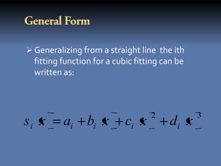
yx a0 a1 x a2 x a3 x
The residual of above equation is
n
R2 [ y (a0 a1 x a 2 x 2 a3 x 3 )] 2 0
i 1](https://image.slidesharecdn.com/n-a-120923061958-phpapp02/85/numarial-analysis-presentation-10-320.jpg)
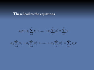
![ Now we take its partial derivatives
The partial derivatives are
n
2
R / a0 2 [y (a 0 a1 x ..... a 3 x 3 )] 0
i 1
n
2
R / a1 2 [y ( a0 a1 x ..... a 3 x 3 )] x 0
i 1
n
R 2 / a2 2 [y (a0 a1 x ..... a 3 x 3 )] x 2 0
i 1
n
2
R / a3 2 [y (a0 a1 x ..... a 3 x 3 )] x 3 0
i 1](https://image.slidesharecdn.com/n-a-120923061958-phpapp02/85/numarial-analysis-presentation-11-320.jpg)


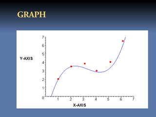


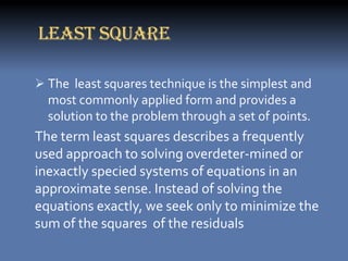
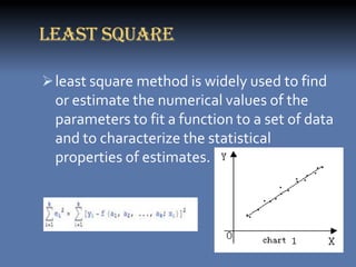
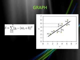
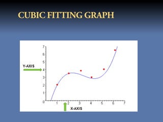
The document discusses the least squares method and cubic fitting method. [1] It explains that least squares finds the best fit curve to a set of data points by minimizing the sum of the squared residuals. [2] Cubic fitting finds the smoothest curve that exactly fits the data points using a cubic polynomial function. [3] An example applies the cubic fitting method to bacterial growth data to determine the parameters for the best fitting cubic curve.


![Mc Ex[1].5 Unit 5 Quadratic Equations](https://cdn.slidesharecdn.com/ss_thumbnails/mcex1-5-unit5quadraticequations-090415020822-phpapp02-thumbnail.jpg?width=640&height=640&fit=bounds)