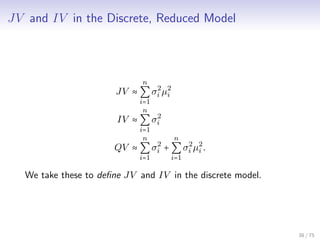
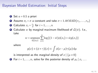
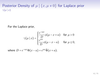
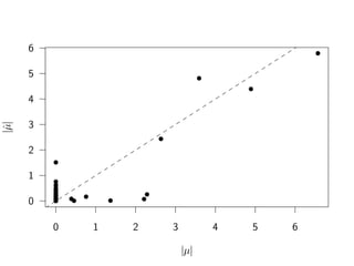
This document outlines a Bayesian model for estimating jump variation in high-frequency asset returns. It begins with background on high-frequency financial data and models jump variation as the sum of squared scaled interval jumps. The continuous jump-diffusion model is reduced to a discrete model where log-returns are modeled as scaled stochastic volatility plus scaled jumps. A Bayesian model is then developed where jumps are modeled with a mixture prior and posterior distributions are derived. Estimation involves calculating posterior jump probabilities and densities. Simulation results demonstrate the model can estimate jump variation.

1. Estimation of Jump Variation in a Bayesian
Model of High-Frequency Asset Returns
Brian Donhauser
Department of Economics
University of Washington
June 14, 2012
1 / 75

2. Outline
Motivation and Previous Work
The Bayesian Model
Jump Variation in the Bayesian Model
Empirical Results
Simulation Results
2 / 75

3. Outline
Motivation and Previous Work
The Bayesian Model
Jump Variation in the Bayesian Model
Empirical Results
Simulation Results
3 / 75

4. Emergence of High-Frequency Financial Data
In the early 1990’s, developments in
the storage and vending of high-frequency financial data and
computing power
laid the groundwork for research in high-frequency finance (Wood,
2000).
4 / 75

5. What to Do With High-Frequency Financial Data?
financial economics: test theoretical market microstructure
models
financial econometrics: model high-frequency prices, volumes,
and durations
estimate lower-frequency quantities (e.g., conditional daily
return variance)
5 / 75

6. 0 100 200 300 400
46.6
46.8
47.0
47.2
47.4
WMT Jan 02, 2008
minutes (t)
prices(St)

7. Simple Returns vs. Log Returns
If St is the spot price of an asset at minute t, then the simple
return over the interval [t − 1,t] is
Rt =
St − St−1
St−1
and the logarithmic return is
rt = log(St) − log(St−1)
= log(1 + Rt)
≈ Rt, for small Rt
We prefer the latter because of additivity and infinite support.
7 / 75

8. A Mathematical Model for an Asset X
X ≡ (Xt)t∈[0,∞)
an adapted, c`adl`ag stochastic process
on a filtered complete probability space (Ω,F,F,P),
satisfying the usual hypothesis
will represent an asset with log-price Xt at time t.
8 / 75

9. Toward a Simple Jump-Diffusion Model for X
Under mild regularity conditions:
rt ≡ Xt − X0 = ∫
t
0
audu + ∫
t
0
σu dWu + Jt, 0 ≤ t < ∞
rt is the log-return over the trading time interval [0,t]
W ∈ BM
a,σ ∈ PRE are the spot drift and spot volatility of returns
Jt = ∑
Nt
i=1 Ci is the cumulative jump process
Nt is a simple counting process of the number of jumps in the
time interval [0,t]
Ci is the size of the ith jump.
9 / 75

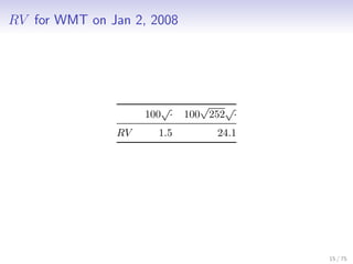
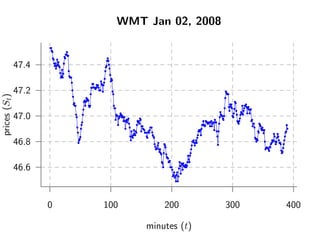
10. Revisiting the Motivating Question
Q: What is the return variance for WMT on January 2nd, 2008?
Q:
Var{rt Ft} =?
where
Ft ≡ F{au,σu}u∈[0,t]
10 / 75

11. Var{r F} = IV
From Andersen et al. (2003, Thm. 2), if (a,σ) W and J ≡ 0,
rt Ft ∼ N (∫
t
0
au du,∫
t
0
σ2
u du)
so
E{rt Ft} = ∫
t
0
au du
Var{rt Ft} = IVt
where
IVt ≡ ∫
t
0
σ2
u dt
11 / 75

12. Realized Variance: RV
For
an asset X
on a time interval [0,t]
with (n + 1)-element partition
Pn ≡ {τ0,τ1,...,τn}, 0 = τ0 ≤ τ1 ≤ ⋯ ≤ τn = t < ∞,
the realized variance
RV
(n)
t ≡
n
∑
i=1
r2
i , 0 ≤ t < ∞
where
ri ≡ Xτi − Xτi−1 , i = 1,...,n
is the i-th log-return on Pn.
12 / 75

13. RV → IV
From Andersen et al. (2003); Barndorff-Nielsen and Shephard
(2002),
RV
(n)
t → IVt
convergence ucp on [0,t]
limit taken over all Pn with limn→∞ Pn = 0.
13 / 75

14. 0 100 200 300 400
46.6
46.8
47.0
47.2
47.4
WMT Jan 02, 2008
minutes (t)
prices(St)

15. RV for WMT on Jan 2, 2008
100
√
⋅ 100
√
252
√
⋅
RV 1.5 24.1
15 / 75

16. 0 10 20 30 40 50 60
20
30
40
50
60
WMT Jan 02, 2008 – Mar 31, 2008
day
AnnualizedVolatilityMeasuresin%

17. Estimating Var{rt Ft} Other Methods
The realized quantity r2
t
GARCH (Bollerslev, 1986)
Stochastic volatility (Melino and Turnbull, 1990; Taylor, 1994;
Harvey et al., 1994; Jacquier et al., 1994)
17 / 75

18. RV → IV + JV
Relaxing J ≡ 0, from Barndorff-Nielsen and Shephard (2004),
RV
(n)
t → IVt + JVt ≈ Var{rt Ft}
where
JVt ≡
Nt
∑
i=1
C2
i .
18 / 75

19. Realized Bipower Variation: RBPV
For
an asset X
on a time interval [0,t]
with (n + 1)-element partition Pn,
the realized bipower variation
RBPV
(n)
t ≡
n
∑
i=2
ri ri−1 , 0 ≤ t < ∞.
19 / 75

20. IVBNS04,JVBNS04
From Barndorff-Nielsen and Shephard (2004), under mild regularity
conditions
IV
(n)
BNS04,t ≡
π
2
RBPV
(n)
t → IVt
JV
(n)
BNS04,t ≡ RV
(n)
t − IV
(n)
BNS04,t → JVt.
20 / 75

21. 0 100 200 300 400
46.6
46.8
47.0
47.2
47.4
WMT Jan 02, 2008
minutes (t)
prices(St)

22. IVBNS04,JVBNS04 for WMT on Jan 2, 2008
100
√
⋅ 100
√
252
√
⋅ %RV
RV 1.5 24.1 100.0
JVBNS04 −0.1 −1.0 −0.2
IVBNS04 1.5 24.1 100.2
22 / 75

23. 0 10 20 30 40 50 60
0
10
20
30
40
50
60
WMT Jan 02, 2008 – Mar 31, 2008
day
AnnualizedVolatilityMeasuresin%

24. Summary of JVBNS04
WMT: Jan 2, 2008 – Mar 31, 2008
100 ∗ (JVBNS04
RV )
Min. −3.5
1st Qu. 1.2
Median 3.6
Mean 4.8
3rd Qu. 8.1
Max. 20.0
24 / 75

25. Simulation Results for JVBNS04: MPE and MAPE
# Jumps
Est. 0 3 10 30
JVBNS04 0.3 −4.5 −12.7 −26.6
IVBNS04 −0.4 4.1 12.7 26.4
# Jumps
Est. 0 3 10 30
JVBNS04 3.3 5.4 12.7 26.6
IVBNS04 6.7 7.3 12.9 26.4
25 / 75

26. Estimating Jump Locations: LM Stat
Extending Barndorff-Nielsen and Shephard, Lee and Mykland
(2008) define their jump statistic
LMl,τi
≡
ri
σi
,
where
σi
2
≡
1
n
IVBNS04,t
and show that jumps are identified with perfect classification
accuracy asymptotically.
26 / 75

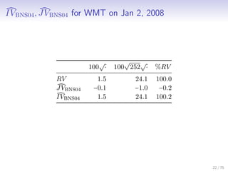
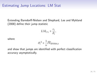
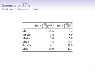
27. Na¨ıve Shrinkage Estimators: JVNS,IVNS
In previous work, I extended Lee and Mykland (2008) and defined
na¨ıve shrinkage estimators of JV, IV
JV
(n)
NS,t ≡
n
∑
i=1
[Fξ(LMg,τi )ri]
2
IV
(n)
NS,t ≡ RV
(n)
t − JVNS,t.
and showed their consistency.
27 / 75

28. 0 100 200 300 400
46.6
46.8
47.0
47.2
47.4
WMT Jan 02, 2008
minutes (t)
prices(St)

29. IVNS,JVNS for WMT on Jan 2, 2008
100
√
⋅ 100
√
252
√
⋅ %RV
RV 1.5 24.1 100.0
JVNS 0.2 3.2 1.7
JVBNS04 −0.1 −1.0 −0.2
IVNS 1.5 23.8 98.3
IVBNS04 1.5 24.1 100.2
29 / 75

30. 0 10 20 30 40 50 60
0
10
20
30
40
50
60
WMT Jan 02, 2008 – Mar 31, 2008
day
AnnualizedVolatilityMeasuresin%

31. 0 10 20 30 40
0
5
10
15
20
WMT Jan 02, 2008 – Mar 31, 2008
100 ∗ JVNS/RV
100∗JVBNS04/RV

32. Summary of JVNS
WMT: Jan 2, 2008 – Mar 31, 2008
100 ∗ (JVBNS04
RV ) 100 ∗ (JVNS
RV )
Min. −3.5 0.4
1st Qu. 1.2 8.9
Median 3.6 15.6
Mean 4.8 16.1
3rd Qu. 8.1 21.9
Max. 20.0 47.1
32 / 75

33. Simulation Results for JVNS: MPE and MAPE
# Jumps
Est. 0 3 10 30
JVNS 1.3 −0.0 −2.1 −10.3
JVBNS04 0.3 −4.5 −12.7 −26.6
IVNS −1.4 −0.4 2.1 10.0
IVBNS04 −0.4 4.1 12.7 26.4
# Jumps
Est. 0 3 10 30
JVNS 1.3 2.7 4.4 10.6
JVBNS04 3.3 5.4 12.7 26.6
IVNS 5.9 5.3 4.7 10.1
IVBNS04 6.7 7.3 12.9 26.4
33 / 75

34. Conclusion: Na¨ıve Shrinkage Estimators
Simulations demonstrate superiority over JVBNS04 :)
Bounded above zero and below RV :)
Non-model-based :(
34 / 75

35. Outline
Motivation and Previous Work
The Bayesian Model
Jump Variation in the Bayesian Model
Empirical Results
Simulation Results
35 / 75

36. Continuous → Discrete: The Reduced Model
Under assumptions and definitions to follow, the continuous
jump-diffusion model reduces to a discrete model where we observe
ri = σixi, with
xi = µi + i, i = 1,...,n,
and
i
i.i.d.
∼ N(0,1) with pdf φ
where µi and σi are unspecified jump and stochastic volatility
processes.
36 / 75

37. Continuous → Discrete: Assumptions and Definitions
Assume,
(i) (Zero Drift). au = 0, ∀u ∈ [0,t],
(ii) (Homogenous Sampling). An (n + 1)-element homogenous
sampling of Xu over the time interval [0,t],
{X0,Xδ,X2δ,...,X(n−1)δ,Xt}, where δ = t/n is the width of
the sampling interval,
and define for i = 1,...,n,
(i) (Interval Volatility). σi ≡ σ[δ(i−1), δi].
(ii) (Scaled Interval Jump). µi ≡ 1
σi
(Jδi − Jδ(i−1)).
(iii) (Log-Returns). ri ≡ Xδi − Xδ(i−1).
(iv) (Scaled Log-Returns). xi ≡ 1
σi
ri.
37 / 75

38. JV and IV in the Discrete, Reduced Model
JV ≈
n
∑
i=1
σ2
i µ2
i
IV ≈
n
∑
i=1
σ2
i
QV ≈
n
∑
i=1
σ2
i +
n
∑
i=1
σ2
i µ2
i .
We take these to define JV and IV in the discrete model.
38 / 75

39. The Discrete Bayesian Model
From Johnstone and Silverman (2004, 2005),
ri = σixi i = 1,...,n, (Observations)
L(xi µi,σi) = φ(xi − µi) i = 1,...,n, (Likelihood)
π(µi) = {
1 − w for µi = 0
wγ(µi) for µi ≠ 0,
i = 1,...,n,
(Prior Jump Density)
w = π {µ ≠ 0}, (Prior Jump Probability)
γ(µ) =
1
2
aexp(−a µ ), (Prior Density of µ {µ ≠ 0})
σi,w,a (Hyperparemeters)
39 / 75

40. Bayesian Model Estimation: Initial Steps
1 Set a = 0.5 a priori
2 Assume σi = σ a constant and take σ = 1.48MAD{r1,...,rn}
3 Calculate xi = ri
σ for i = 1,...,n
4 Calculate w by marginal maximum likelihood of L( ˇw). I.e.,
take
w = argmax
0≤ ˇw≤1
n
∑
i=1
log{(1 − ˇw)φ(xi) + ˇwg(xi)}
where
g(x) ≡ (φ ∗ γ)(x) ≡ ∫ φ(x − µ)γ(µ)dµ
is interpreted as the marginal density of x {µ ≠ 0}
5 For i = 1,...,n, solve for the posterior density of µi xi . . .
40 / 75

41. Posterior Density of µ x
π(µ x)
After much algebra, we can write the posterior density of µ x as
π(µ x) = {
1 − w(x) for µ = 0
w(x)γ(µ x) for µ ≠ 0,
where γ(µ x) is the posterior density of µ {x,µ ≠ 0} and
w(x) ≡ π(µ ≠ 0 x) is the posterior non-zero jump probability
41 / 75

42. Posterior Density of µ {x,µ ≠ 0} for Laplace prior
γ(µ x)
For the Laplace prior,
γ(µ x) =
⎧⎪⎪⎪⎪⎪
⎨
⎪⎪⎪⎪⎪⎩
e−ax
D
φ(µ − x + a) for µ > 0
eax
D
φ(µ − x − a) for µ ≤ 0,
where D = e−ax
Φ(x − a) + eax ˜Φ(x + a).
42 / 75

43. Posterior Density Illustration
From Johnstone (2011):
43 / 75

44. Posterior Mean of µ x for Laplace Prior
ˆµπ(x)
Recall the posterior density of µ x is given by
π(µ x) = {
1 − w(x) for µ = 0
w(x)γ(µ x) for µ ≠ 0.
Then the posterior mean of µ x is
ˆµπ(x) = w(x)ˆµγ(x)
= w(x)
→1
(x − a
{e−ax
Φ(x − a) − eax ˜Φ(x + a)}
e−axΦ(x − a) + eax ˜Φ(x + a)
)
→(x−a)
→ x − a for large x
in the case of Laplace prior density γ(µ)
44 / 75

45. 0 50 100 150 200 250
-2
0
2
4
6
i
xi,µi,ˆµ(xi)

46. 0 1 2 3 4 5 6
0
1
2
3
4
5
6
µ
ˆµ

47. Outline
Motivation and Previous Work
The Bayesian Model
Jump Variation in the Bayesian Model
Empirical Results
Simulation Results
47 / 75

48. Posterior Mean of JV x: Na¨ıve Approach
JVNEB, 2 (x)
Recall that
JV ≡
n
∑
i=1
σ2
i µ2
i .
Then, a na¨ıve estimation approach gives
JVNEB, 2 (x) ≡
n
∑
i=1
σ2
i ˆµπ,i(xi)2
.
From Jensen’s inequality we expect this to under-represent the
actual posterior mean of JV : JVEB, 2 (x). But, very easy to
calculate!
48 / 75

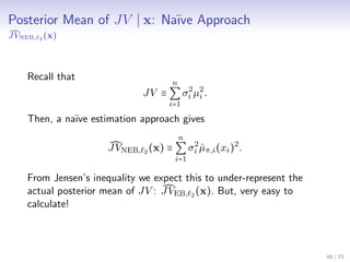
49. Posterior Mean of JV x: Na¨ıve Relation
JVEB, 2 (x)
JVEB, 2 (x) ≡ E[JV x]
= E[
n
∑
i=1
σ2
i µ2
i x]
=
n
∑
i=1
σ2
i E[µ2
i xi]
=
n
∑
i=1
σ2
i ˆµπ,i(xi)2
+ σ2
i Var[µi xi]
= JVNEB, 2 (x) +
n
∑
i=1
σ2
i Var[µi xi].
49 / 75

50. Posterior Mean of JV x for Laplace Prior
JVEB, 2 (x)
So then,
JVEB, 2 (x) =
n
∑
i=1
σ2
i µ2
π,i(xi)
where, after skipping a large amount of algebra,
µ2
π(x) = w(x)µ2
γ(x)
= w(x)(x2
+ a2
+ 1 − 2ax{
e−ax
Φ(x − a) − eax ˜Φ(x + a)
D
}
−2a{
e−ax
φ(x − a)
D
})
→ (x − a)2
+ 1 for large x
= ˆµπ(x)2
+ 1 for large x
for the Laplace prior. Closed form!
50 / 75

51. Posterior Median of JV x for Laplace Prior
JVEB, 1 (x)
No simple closed form result. Can still get a numerical result via
the following procedure:
1 Simulate one value µi,1 from each of the n posterior jump
densities πi(µi xi)
2 Calculate JV1 = ∑n
i=1 σ2
i µ2
i,1
3 Repeat steps 1-2 k-times, returning {JV1,...,JVk}
4 Then, for large k, JVEB, 1 (x) ≈ Median{JV1,...,JVk}
51 / 75

52. Outline
Motivation and Previous Work
The Bayesian Model
Jump Variation in the Bayesian Model
Empirical Results
Simulation Results
52 / 75

53. 0 100 200 300 400
46.6
46.8
47.0
47.2
47.4
WMT Jan 02, 2008
minutes (t)
prices(St)

54. JVEB, 2
for WMT on Jan 2, 2008
Window 100
√
⋅ 100
√
252
√
⋅ %RV
JVEB, 2 full 0.8 12.1 25.4
60min 0.7 11.7 23.8
30min 0.6 8.7 13.2
15min 0.5 8.4 12.1
10min 0.6 9.4 15.3
05min 0.7 11.6 23.3
IVEB, 2 full 1.3 20.8 74.6
60min 1.3 21.0 76.2
30min 1.4 22.4 86.8
15min 1.4 22.6 87.9
10min 1.4 22.1 84.7
05min 1.3 21.1 76.7
54 / 75

55. IVEB,JVEB for WMT on Jan 2, 2008
100
√
⋅ 100
√
252
√
⋅ %RV
RV 1.5 24.1 100.0
JVEB, 1 0.5 8.5 12.5
JVEB, 2 0.6 8.7 13.2
JVNS 0.2 3.2 1.7
JVBNS04 −0.1 −1.0 −0.2
IVEB, 1 1.4 22.5 87.5
IVEB, 2 1.4 22.4 86.8
IVNS 1.5 23.8 98.3
IVBNS04 1.5 24.1 100.2
55 / 75

56. 0 10 20 30 40 50 60
0
10
20
30
40
50
60
WMT Jan 02, 2008 – Mar 31, 2008
day
AnnualizedVolatilityMeasuresin%

57. 0 10 20 30 40 50
0
5
10
15
20
WMT Jan 02, 2008 – Mar 31, 2008
100 ∗ JVEB, 2 /RV
100∗JVBNS04/RV

58. 0 10 20 30 40 50
0
10
20
30
40
WMT Jan 02, 2008 – Mar 31, 2008
100 ∗ JVEB, 2 /RV
100∗JVNS/RV

59. Summary of JVEB, 2
WMT: Jan 2, 2008 – Mar 31, 2008
100 ∗ (JVBNS04
RV ) 100 ∗ (JVNS
RV ) 100 ∗ (
JVEB, 2
RV )
Min. −3.5 0.4 0.0
1st Qu. 1.2 8.9 19.4
Median 3.6 15.6 25.6
Mean 4.8 16.1 26.3
3rd Qu. 8.1 21.9 33.0
Max. 20.0 47.1 52.7
59 / 75

60. Outline
Motivation and Previous Work
The Bayesian Model
Jump Variation in the Bayesian Model
Empirical Results
Simulation Results
60 / 75

61. Simulation Model
(Number of Observations). n = 390.
(Observations). For i = 1,...,n,
ri = σixi,
where
xi = µi + i, i
i.i.d.
∼ N(0,1).
(Interval Volatility). σi = σ = 0.000638 ≈ 0.20/
√
252 ∗ 390.
(Scaled Jumps). µi µi ≠ 0 ∼ U(−s,s), with s
deterministically set equal to 4, 7, 10, and 15.
(Number of Jumps). Deterministically set equal to 0, 3, 10,
and 30.
(Jump Locations). Each uniformly chosen from i = 1,...,n
(Number of Simulations). m = 5000
61 / 75

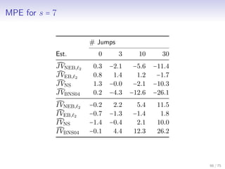
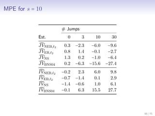
62. Estimator Evaluation Criteria: MPE, MAPE
We define the mean percentage error and mean absolute
percentage error for an estimator JV of JV as
MPE(JV ) = 100 ∗ E[
JV − JV
QV
]
MAPE(JV ) = 100 ∗ E[
JV − JV
QV
]
and similarly for an estimator IV of IV
MPE(IV ) = 100 ∗ E[
IV − IV
QV
]
MAPE(IV ) = 100 ∗ E[
IV − IV
QV
]
62 / 75

63. Estimator Evaluation Criteria: Sample MPE and MAPE
We approximate MPE and MAPE by their sample counterparts
MPE(JV ) ≈
100
m
m
∑
j=1
JVj − JVj
QVj
MAPE(JV ) ≈
100
m
m
∑
j=1
JVj − JVj
QVj
MPE(IV ) ≈
100
m
m
∑
j=1
IVj − IVj
QVj
MAPE(IV ) ≈
100
m
m
∑
j=1
IVj − IVj
QVj
63 / 75

64. MPE for s = 4
# Jumps
Est. 0 3 10 30
JVNEB, 2 0.3 −2.1 −6.5 −15.5
JVEB, 2 0.8 −0.4 −2.1 −6.3
JVNS 1.3 −0.5 −4.0 −15.1
JVBNS04 0.2 −2.0 −7.3 −19.1
IVNEB, 2 −0.2 2.0 6.9 15.6
IVEB, 2 −0.7 0.3 2.5 6.4
IVNS −1.4 0.1 3.9 14.8
IVBNS04 −0.1 1.9 7.7 19.1
64 / 75

65. MAPE for s = 4
# Jumps
Est. 0 3 10 30
JVNEB, 2 0.3 2.7 6.8 15.5
JVEB, 2 0.8 3.3 5.6 8.5
JVNS 1.3 2.1 4.8 15.1
JVBNS04 3.3 3.7 7.6 19.1
IVNEB, 2 5.8 5.9 7.9 15.7
IVEB, 2 6.0 6.2 6.7 8.5
IVNS 5.9 5.7 6.4 14.9
IVBNS04 6.7 6.4 8.7 19.2
65 / 75

66. MPE for s = 7
# Jumps
Est. 0 3 10 30
JVNEB, 2 0.3 −2.1 −5.6 −11.4
JVEB, 2 0.8 1.4 1.2 −1.7
JVNS 1.3 −0.0 −2.1 −10.3
JVBNS04 0.2 −4.3 −12.6 −26.1
IVNEB, 2 −0.2 2.2 5.4 11.5
IVEB, 2 −0.7 −1.3 −1.4 1.8
IVNS −1.4 −0.4 2.1 10.0
IVBNS04 −0.1 4.4 12.3 26.2
66 / 75

67. MAPE for s = 7
# Jumps
Est. 0 3 10 30
JVNEB, 2 0.3 3.3 6.3 11.4
JVEB, 2 0.8 3.9 4.8 4.7
JVNS 1.3 2.7 4.4 10.6
JVBNS04 3.3 5.3 12.6 26.1
IVNEB, 2 5.8 5.8 6.5 11.5
IVEB, 2 6.0 6.1 5.1 3.7
IVNS 5.9 5.3 4.7 10.1
IVBNS04 6.7 7.3 12.6 26.2
67 / 75

68. MPE for s = 10
# Jumps
Est. 0 3 10 30
JVNEB, 2 0.3 −2.3 −6.0 −9.6
JVEB, 2 0.8 1.4 −0.1 −2.7
JVNS 1.3 0.2 −1.0 −6.4
JVBNS04 0.2 −6.3 −15.6 −27.4
IVNEB, 2 −0.2 2.3 6.0 9.8
IVEB, 2 −0.7 −1.4 0.1 2.9
IVNS −1.4 −0.6 1.0 6.1
IVBNS04 −0.1 6.3 15.5 27.7
68 / 75

69. MAPE for s = 10
# Jumps
Est. 0 3 10 30
JVNEB, 2 0.3 3.9 6.5 9.7
JVEB, 2 0.8 4.0 4.2 4.3
JVNS 1.3 3.1 4.2 6.9
JVBNS04 3.3 7.1 15.6 27.4
IVNEB, 2 5.8 5.0 6.3 9.8
IVEB, 2 6.0 5.1 3.6 3.3
IVNS 5.9 4.8 3.5 6.2
IVBNS04 6.7 7.8 15.6 27.7
69 / 75

70. MPE for s = 15
# Jumps
Est. 0 3 10 30
JVNEB, 2 0.3 −2.7 −5.4 −7.9
JVEB, 2 0.8 0.6 −1.3 −4.0
JVNS 1.3 0.2 −0.4 −3.7
JVBNS04 0.2 −7.8 −16.0 −25.0
IVNEB, 2 −0.2 2.7 5.4 7.9
IVEB, 2 −0.7 −0.6 1.3 4.0
IVNS −1.4 −0.6 0.4 3.5
IVBNS04 −0.1 7.8 16.0 25.0
70 / 75

71. MAPE for s = 15
# Jumps
Est. 0 3 10 30
JVNEB, 2 0.3 4.3 6.0 7.9
JVEB, 2 0.8 4.1 4.0 4.5
JVNS 1.3 3.6 3.8 4.5
JVBNS04 3.3 8.4 16.0 25.0
IVNEB, 2 5.8 4.5 5.5 7.9
IVEB, 2 6.0 4.1 2.6 4.0
IVNS 5.9 3.9 2.2 3.6
IVBNS04 6.7 8.8 16.0 25.0
71 / 75

72. Conclusion: Empirical Bayesian Estimators
Simulations demonstrate superiority over JVBNS04 and JVNS
:)
Model-based :)
Bounded above zero :)
Not necessarily bounded below RV :(
May depend on window of volatility estimation :(
72 / 75

73. Bibliography I
Andersen, T., T. Bollerslev, F. Diebold, and P. Labys (2003).
Modeling and forecasting realized volatility.
Econometrica 71(2), 579–625.
Barndorff-Nielsen, O. and N. Shephard (2002). Econometric
analysis of realized volatility and its use in estimating stochastic
volatility models. Journal of the Royal Statistical Society. Series
B (Statistical Methodology) 64(2), 253–280.
Barndorff-Nielsen, O. E. and N. Shephard (2004). Power and
bipower variation with stochastic volatility and jumps. Journal of
Financial Econometrics 2(1), 1–37.
Barndorff-Nielsen, O. E. and N. Shephard (2006). Econometrics of
testing for jumps in financial economics using bipower variation.
Journal of Financial Econometrics 4(1), 1–30.
Bollerslev, T. (1986). Generalized autoregressive conditional
heteroskedasticity. Journal of econometrics 31(3), 307–327.
73 / 75

74. Bibliography II
Harvey, A., E. Ruiz, and N. Shephard (1994). Multivariate
stochastic variance models. The Review of Economic
Studies 61(2), 247–264.
Jacquier, E., N. Polson, and P. Rossi (1994). Bayesian analysis of
stochastic volatility models. Journal of Business & Economic
Statistics 12(4), 371–389.
Johnstone, I. and B. Silverman (2005). Ebayesthresh: R programs
for empirical bayes thresholding. Journal of Statistical
Software 12(8), 1–38.
Johnstone, I. M. (2011). Gaussian estimation: Sequence and
multiresolution models.
Johnstone, I. M. and B. W. Silverman (2004). Needles and straw
in haystacks: Empirical bayes estimates of possibly sparse
sequences. The Annals of Statistics 32(4), 1594–1649.
74 / 75

75. Bibliography III
Lee, S. S. and P. A. Mykland (2008). Jumps in financial markets:
A new nonparametric test and jump dynamics. Review of
Financial studies 21(6), 2535–2563.
Melino, A. and S. Turnbull (1990). Pricing foreign currency
options with stochastic volatility. Journal of
Econometrics 45(1-2), 239–265.
Taylor, S. (1994). Modeling stochastic volatility: A review and
comparative study. Mathematical finance 4(2), 183–204.
Wood, R. (2000). Market microstructure research databases:
History and projections. Journal of Business & Economic
Statistics, 140–145.
75 / 75