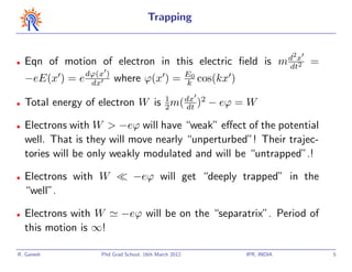
This document discusses the breakdown of linearization in the Vlasov equation due to particle trapping in an oscillating electric field. It shows that the linear Landau damping solution is only valid when the perturbation amplitude is small and for times less than the trapping time scale τtr. Beyond τtr, particles become trapped in oscillation in the electric potential well, violating the assumption of unperturbed trajectories used in the linearized solution. Nonlinear effects then dominate and nonlinear methods are required.

1. Vlasov Equation - Trapping, Break Down of Linearization &
Nonlinearity
R. Ganesh
Institute for Plasma Research, Bhat, INDIA
Major References
Intro. to Plasma Physics-F.F.Chen,
Intro. to Plasma Physics-R. J. Goldston & P.H Rutherford,
Fundamentals of Plasma Physics-P.M.Bellan
R. Ganesh Phd Grad School, 16th March 2012 IPR, INDIA 1

2. Outline
• Travelling wave electric field, Trapping-Oscillations
R. Ganesh Phd Grad School, 16th March 2012 IPR, INDIA 2

3. Vlasov-Maxwell Eqns
• Collisionless, Vlasov Eqn is :
∂ ∂ q ∂
∂t f (x, v, t) + v · ∂x f (x, v, t) + m E(x, t) · ∂v f (x, v, t) = 0 for each
species
• Maxwell’s Eqns
q
• For example, for an electrostaic problem ·E = 0
ρ(x, t)
• For linearizing Vlasov Eqn, amplitude of the perturbation in
space should be small.
• Also “smallness” of f1(x, v, t) in v. That is, | ∂f1(x,v,t) |
∂v
| ∂f∂v |.
0 (v)
R. Ganesh Phd Grad School, 16th March 2012 IPR, INDIA 3

4. Trapping
• In the Initial Value Approach, the solution of Linearized Vlasov
Eqn was obtained by “following f1” along the “unperturbed
trajectories of particles”.
• “Unperturbed trajectories” implies the equilibrium trajectories
of particles as if the perturbation does not “backreact”on the
trajectories of particles. This limit is the linear limit.
• Now let us consider a travelling wave E(x, t) = E0 sin(kx − ωt)
in a uniform warm plasma.
• When one moves with the phase velocity of the wave, there
won’t be any explicit time dependence! i.e, E0 sin(kx ) in a
frame moving with ω/k!!
R. Ganesh Phd Grad School, 16th March 2012 IPR, INDIA 4

5. Trapping
d2x
• Eqn of motion of electron in this electric field is m dt2 =
−eE(x ) = e dϕ(x ) where ϕ(x ) =
dx
E0
k cos(kx )
• Total energy of electron W is 1 m( dx )2 − eϕ = W
2 dt
• Electrons with W > −eϕ will have “weak” effect of the potential
well. That is they will move nearly “unperturbed”! Their trajec-
tories will be only weakly modulated and will be “untrapped”.!
• Electrons with W −eϕ will get “deeply trapped” in the
“well”.
• Electrons with W −eϕ will be on the “separatrix”. Period of
this motion is ∞!
R. Ganesh Phd Grad School, 16th March 2012 IPR, INDIA 5

6. Trapping...
• Eqn of motion for such “deeply trapped” particles, the amplitude
“ x’ ” of oscillation will be small and hence “sin” can be expanded
d2x 2
to get m dt2 = −eE0 sin(kx ) −eE0kx = −mωtr x where
eE0k −1 m
ωtr = m or τtr ωtr = eE0k
• This is harmonic motion in which trajectories of particles are
so heavily distorted and no more remain “unperturbed” by the
field!
• This implies that the approximation of “linearity” of Vlasov
Eqn as treated for Landau damping (along the unperturbed
m
trajectories) will be valid for times τL τtr = eE0k
R. Ganesh Phd Grad School, 16th March 2012 IPR, INDIA 6

7. Trapping...
• This implies that Linear Landau Damping is valid for very small
values of E0 - i.e., very small amplitude waves!
−1
• The above condition says τL γL τtr !
• Beyond this time scale, nonlinear effects dominate and one has
to abondon linear methods.
R. Ganesh Phd Grad School, 16th March 2012 IPR, INDIA 7

8. Landau Damping Initial Value Problem - Recollect
• Equilibrium: Unmagnetized plasma (B0 = 0), a unif. distribution
of electrons (e) and ions (i). For simplicity consider a 1D problem
along x. Electrons are mobile & ions at rest.
• No equilibrium electric field (field free equilibrium)
∂
•
∂t ≡ 0, equilibrium electric field E0 = 0. What is the equilibrium
distribution f0 like?
• Vlasav Eqn becomes v ∂f0∂x = 0 which implies that f0 = f0(v).
(x,v)
As equil.distn is independent of x, equilibrium density n0 is
uniform such that f0(v)dv = n0.
• Perturbation : f (x, v, t) = f0(v) + f1(x, v, t) i.e, ampl. is small.
Similarly E(x, t) = 0 + E1(x, t).
R. Ganesh Phd Grad School, 16th March 2012 IPR, INDIA 8

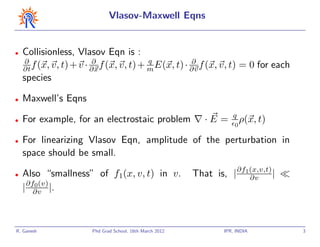
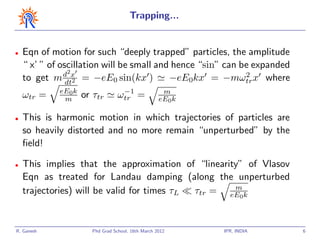
9. Landau Damping I.V. Problem contd..
∂ ∂ e ∂
•
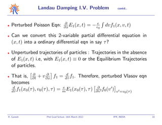
∂t [f0(v)+f1(x, v, t)]+v ∂x [f0(v)+f1(x, v, t)]− m E1(x, t) ∂v [f0(v)+
f1(x, v, t)] = 0
∂ e
• Poisson Eqn: ∂x E1(x, t) = 0
n0 − dv[f0(v) + f1(x, v, t)]
∂ ∂
• Zeroth Order Vlasov Eqn: ∂t f0(v) + v ∂x f0(v) = 0
∂ ∂ e ∂
• 1st Order: ∂t + v ∂x f1(x, v, t) = m E1(x, t) ∂v f0(v)
R. Ganesh Phd Grad School, 16th March 2012 IPR, INDIA 9

10. Landau Damping I.V. Problem contd..
∂
• Perturbed Poisson Eqn: ∂x E1(x, t) = − e0 dvf1(x, v, t)
• Can we convert this 2-variable partial differential equation in
(x, t) into a ordinary differential eqn in say τ ?
• Unperturbed trajectories of particles : Trajectories in the absence
of E1(x, t) i.e, with E1(x, t) ≡ 0 or the Equilibrium Trajectories
of particles.
∂ ∂ d
• That is, ∂t + v ∂x f1 = dτ f1. Therefore, perturbed Vlasov eqn
becomes
d e ∂
dτ f1(x0(τ ), v0(τ ), τ ) = m E1(x0(τ ), τ ) ∂v f0(v ) v =v (τ )
0
R. Ganesh Phd Grad School, 16th March 2012 IPR, INDIA 10

11. Landau Damping I.V. Problem contd..
• If we represent equilibrium trajectories with x0(τ ) and v0(τ ),
then dxdτ ) = v0(τ ) and dvdτ ) = 0
0 (τ 0 (τ
• If x0(τ = t) = x and v0(τ = t) = v, then solving trajectories
yields x0(τ ) = x + v(τ − t) and v0(τ ) = v
• Now, the total derivative in τ can be integrated from τ = 0
to τ = t, i.e, f1(x, v, t) = f1(x0(τ = 0), v0(τ = 0), τ = 0) +
e t ∂
m 0 dτ E1(x0(τ ), τ ) ∂v f0(v ) v =v (τ )
0
• When we put back the trajectories we get f1(x, v, t) = f1(x −
e ∂ t
vt, v, 0) + m ∂v f0(v) 0 dτ E1(x + v(τ − t), τ )
• Substituting in Poisson Eqn gives the dispersion.
R. Ganesh Phd Grad School, 16th March 2012 IPR, INDIA 11

12. Break Down of Linear Landau Damping contd..
• Now consider our perturbation for E1(x, t) = E0 sin(kx − ωt)
• Consistent to this perturbation, let us consider an initial value
for f1(x, v, 0) = f1(v, 0) cos(kx)
• Solution of the Vlasov Eqn f1(x, v, t) solved above using method
of unperturbed trajectories is f1(x, v, t) = f1(v, 0) cos(kx −
e ∂ t
kvt) + m ∂v f0(v) 0 dτ E0 sin(k(x + v(τ − t)) − ωt)
• Integration in time yields f1(x, v, t) = f1(v, 0) cos(kx − kvt) +
e ∂
m ∂v f0(v)E0 cos(kx−ωt)−cos(kx−kvt)
ω−kv
• Expanding cos terms around v = ω/k gives f1(x, v, t) =
e ∂
f1(v, 0) cos(kx − kvt) + m ∂v f0(v)E0 ×
t2
t sin(kx − ωt) + 2 (ω − kv) cos(kx − kvt)
R. Ganesh Phd Grad School, 16th March 2012 IPR, INDIA 12

13. Break Down of Linear Landau Damping contd..
• Expanding cos terms around v = ω/k gives f1(x, v, t) =
e ∂
f1(v, 0) cos(kx − kvt) + m ∂v f0(v)E0 ×
t2
t sin(kx − ωt) + 2 (ω − kv) cos(kx − kvt)
• Taking a derivative of the solution w.r.t v, and evaluating around
v = ω/k and keeping dominant contribution for large t,
∂f1 ∂f0(v) eE0k t2
∂v = − ∂v m 2 cos(kx − ωt)
v=ω/k
• Condition for validity of linear approximation, namely
m
|∂f1/∂v| |∂f0/∂v| breaks down for t ekE0 τtr
• The secular term and divergence beyond t > τtr because “un-
perturbed trajectories” (x − vt) breaks down due to trapping!
• Hence nonlinear methods will have to be used.
R. Ganesh Phd Grad School, 16th March 2012 IPR, INDIA 13