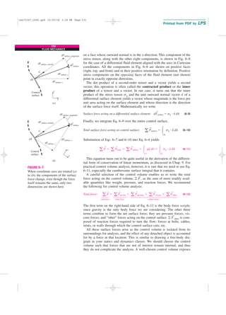
1) The document discusses momentum analysis of fluid flow systems using control volume analysis. It provides background on Newton's laws of motion and conservation of linear and angular momentum.
2) Control volume analysis using the linear momentum and angular momentum equations allows determining the forces and torques associated with fluid flow into and out of a control volume.
3) The key forces acting on a control volume are body forces that act throughout the volume, like gravity, and surface forces that act on the control surface, like pressure and viscous forces.


 ⫽ 23.56 kg/s
256
FLUID MECHANICS
cen72367_ch06.qxd 10/29/04 2:26 PM Page 256](https://image.slidesharecdn.com/momentumequation-220921100120-f930d981/85/Momentum-equation-pdf-30-320.jpg)
![or
Discussion Note that the pipe weight and the momentum of the exit stream
cause opposing moments at point A. This example shows the importance of
accounting for the moments of momentums of flow streams when performing
a dynamic analysis and evaluating the stresses in pipe materials at critical
cross sections.
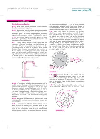
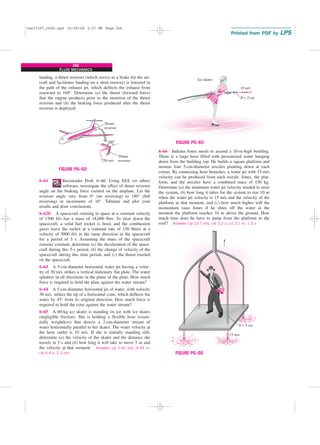
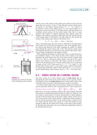
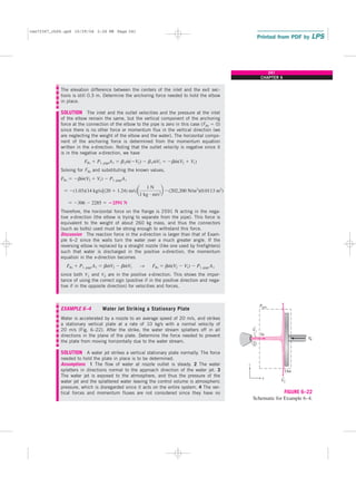
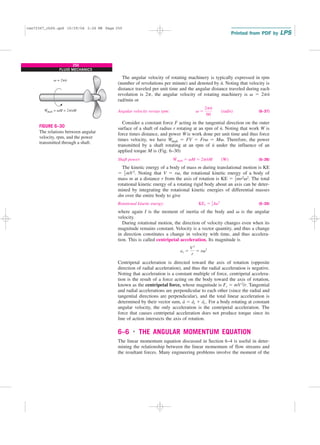
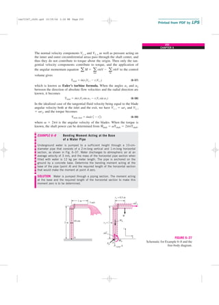
EXAMPLE 6–9 Power Generation from a Sprinkler System
A large lawn sprinkler with four identical arms is to be converted into a tur-
bine to generate electric power by attaching a generator to its rotating head,
as shown in Fig. 6–38. Water enters the sprinkler from the base along the
axis of rotation at a rate of 20 L/s and leaves the nozzles in the tangential
direction. The sprinkler rotates at a rate of 300 rpm in a horizontal plane.
The diameter of each jet is 1 cm, and the normal distance between the axis
of rotation and the center of each nozzle is 0.6 m. Estimate the electric
power produced.
SOLUTION A four-armed sprinkler is used to generate electric power. For a
specified flow rate and rotational speed, the power produced is to be deter-
mined.
Assumptions 1 The flow is cyclically steady (i.e., steady from a frame of ref-
erence rotating with the sprinkler head). 2 The water is discharged to the
atmosphere, and thus the gage pressure at the nozzle exit is zero. 3 Genera-
tor losses and air drag of rotating components are neglected. 4 The nozzle
diameter is small compared to the moment arm, and thus we use average
values of radius and velocity at the outlet.
Properties We take the density of water to be 1000 kg/m3 ⫽ 1 kg/L.
Analysis We take the disk that encloses the sprinkler arms as the control
volume, which is a stationary control volume.
The conservation of mass equation for this steady-flow system is m
.
1 ⫽ m
.
2
⫽ m
.
total. Noting that the four nozzles are identical, we have m
.
nozzle ⫽ m
.
total/4
or V
.
nozzle ⫽ V
.
total/4 since the density of water is constant. The average jet
exit velocity relative to the nozzle is
Vjet ⫽
V
#
nozzle
Ajet
⫽
5 L/s
[p(0.01 m)2
/4]
a
1 m3
1000 L
b ⫽ 63.66 m/s
L ⫽
B
2r2m
#
V2
w
⫽
B
2 ⫻ 141.4 N ⭈ m
118 N/m
⫽ 2.40 m
257
CHAPTER 6
r = 0.6 m
mtotal
Electric
generator
v
Tshaft
mnozzle
⋅
r
⋅
⋅
r
mnozzle
⋅
r
jet
V
jet
V
jet
V
jet
V
V
V
V
V
mnozzle
⋅
r
mnozzle
FIGURE 6–38
Schematic for Example 6–9 and the
free-body diagram.
cen72367_ch06.qxd 10/29/04 2:26 PM Page 257](https://image.slidesharecdn.com/momentumequation-220921100120-f930d981/85/Momentum-equation-pdf-31-320.jpg)