Download as PDF, PPTX


![• Scalar fields
As in the flat space time, each real scalar field operator
is decomposed as
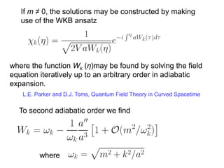
The function χk(η) satisfies the field equation
Where ’ denotes a derivative with respect to the
conformal time η .
[N.D. Birell, P.C.W. Davies, Quantum Fields in Curved Space]](https://image.slidesharecdn.com/bw2011-31-bilic-110911100507-phpapp01/85/N-Bilic-Supersymmetric-Dark-Energy-32-320.jpg)
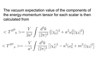
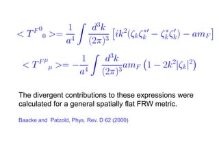
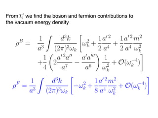
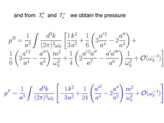
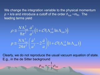


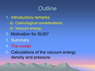
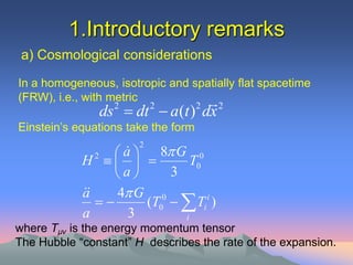
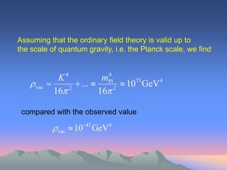
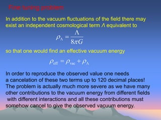
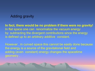
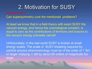
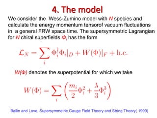
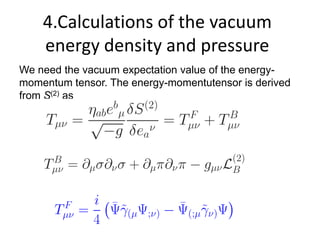
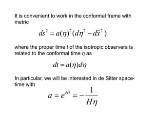
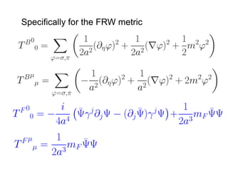
This document discusses the relationship between supersymmetry (SUSY) and vacuum energy density in cosmology, particularly addressing the vacuum energy problem and the role of a nonzero cosmological constant. It outlines how SUSY can potentially provide a solution to issues related to the vast discrepancy between theoretical and observed vacuum energy values. The model emphasizes the interconnection between vacuum fluctuations, dark energy, and effective equation of state equations, with considerations on the implications for cosmic expansion.