Download to read offline


![Nonlocal
cosmology
Ivan Dimitrijevi´c
References
Dimitrijevic, I., Dragovich, B., Grujic J., Rakic, Z.: New
cosmological solutions in nonlocal modified gravity. Rom. Journ.
Phys. 58 (5-6), 550559 (2013) [arXiv:1302.2794 [gr-qc]]
I. Dimitrijevic, B.Dragovich, J. Grujic, Z. Rakic, “A new model of
nonlocal modified gravity”, Publications de l’Institut Mathematique
94 (108), 187–196 (2013).
Ivan Dimitrijevic, Branko Dragovich, Jelena Grujic, and Zoran Rakic.
On Modified Gravity. Springer Proc.Math.Stat., 36:251-259, 2013.
I. Dimitrijevic, B. Dragovich, J. Grujic, and Z. Rakic. Some
power-law cosmological solutions in nonlocal modified gravity. In Lie
Theory and Its Applications in Physics, volume 111 of Springer
Proceedings in Mathematics and Statistics, pages 241-250, 2014.
I. Dimitrijevic, B. Dragovich, J. Grujic, and Z. Rakic. Some
cosmological solutions of a nonlocal modified gravity. Filomat, 2014.](https://image.slidesharecdn.com/dimitrijevic-i-180626175257/85/Ivan-Dimitrijevic-Nonlocal-cosmology-37-320.jpg)


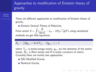
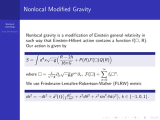
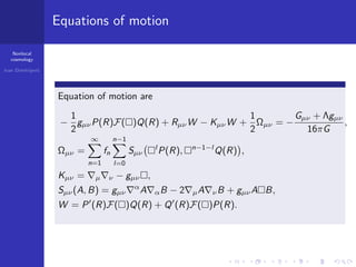
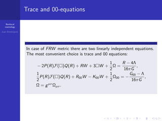
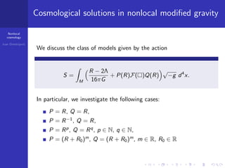
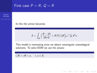
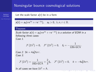
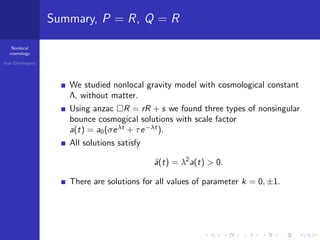
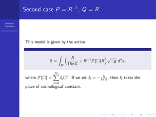
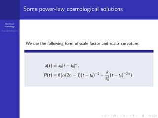
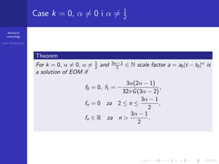
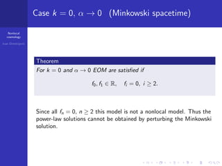
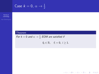
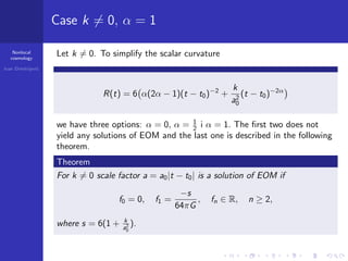
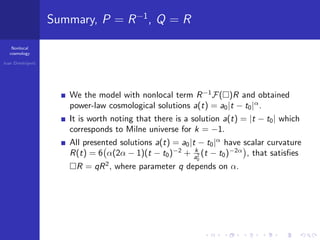
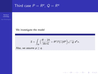
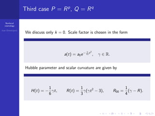
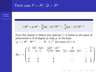
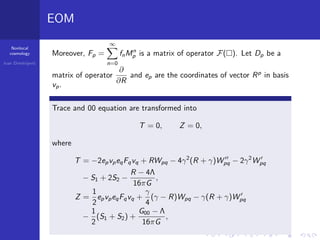
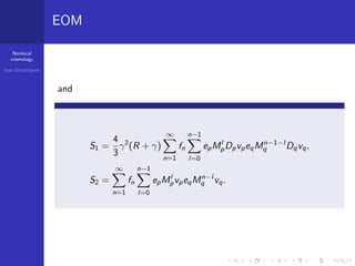
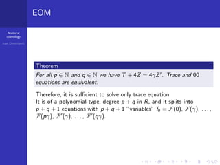
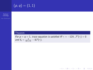
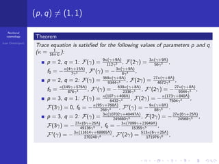
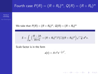
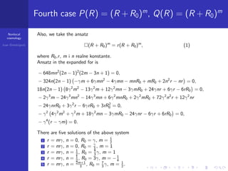
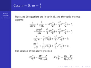
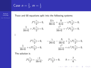
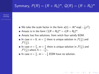
This document discusses nonlocal cosmology and modifications to Einstein's theory of gravity. It presents three cases of nonlocal modified gravity models: 1. When P(R)=R and Q(R)=R, nonsingular bounce cosmological solutions were found with scale factor a(t)=a0(σeλt+τe-λt). 2. When P(R)=R-1 and Q(R)=R, several power-law cosmological solutions were obtained, including a(t)=a0|t-t0|α. 3. For the case P(R)=Rp and Q(R)=Rq, the trace and 00 equations of motion were transformed into an equivalent


![NCTS--FGCPA-LeCosPA-[Kazuharu-Bamba].pdf](https://cdn.slidesharecdn.com/ss_thumbnails/ncts-fgcpa-lecospa-kazuharu-bamba-240912175320-cc36fa15-thumbnail.jpg?width=640&height=640&fit=bounds)


![Polymer [ बहुलक ] Chemistry Notes PDF - Irfanullah Mehar - JJ Sir Chemistry.pdf](https://cdn.slidesharecdn.com/ss_thumbnails/polymerchemistrynotespdf-irfanullahmehar-jjsirchemistry-260210172118-3f9b37f7-thumbnail.jpg?width=640&height=640&fit=bounds)


