Download as PDF, PPTX
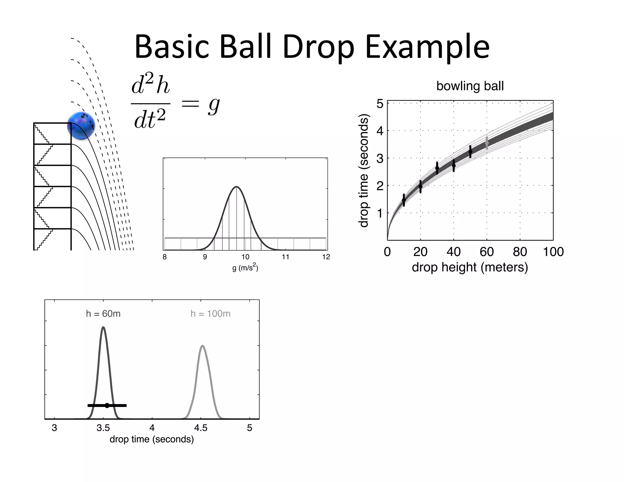
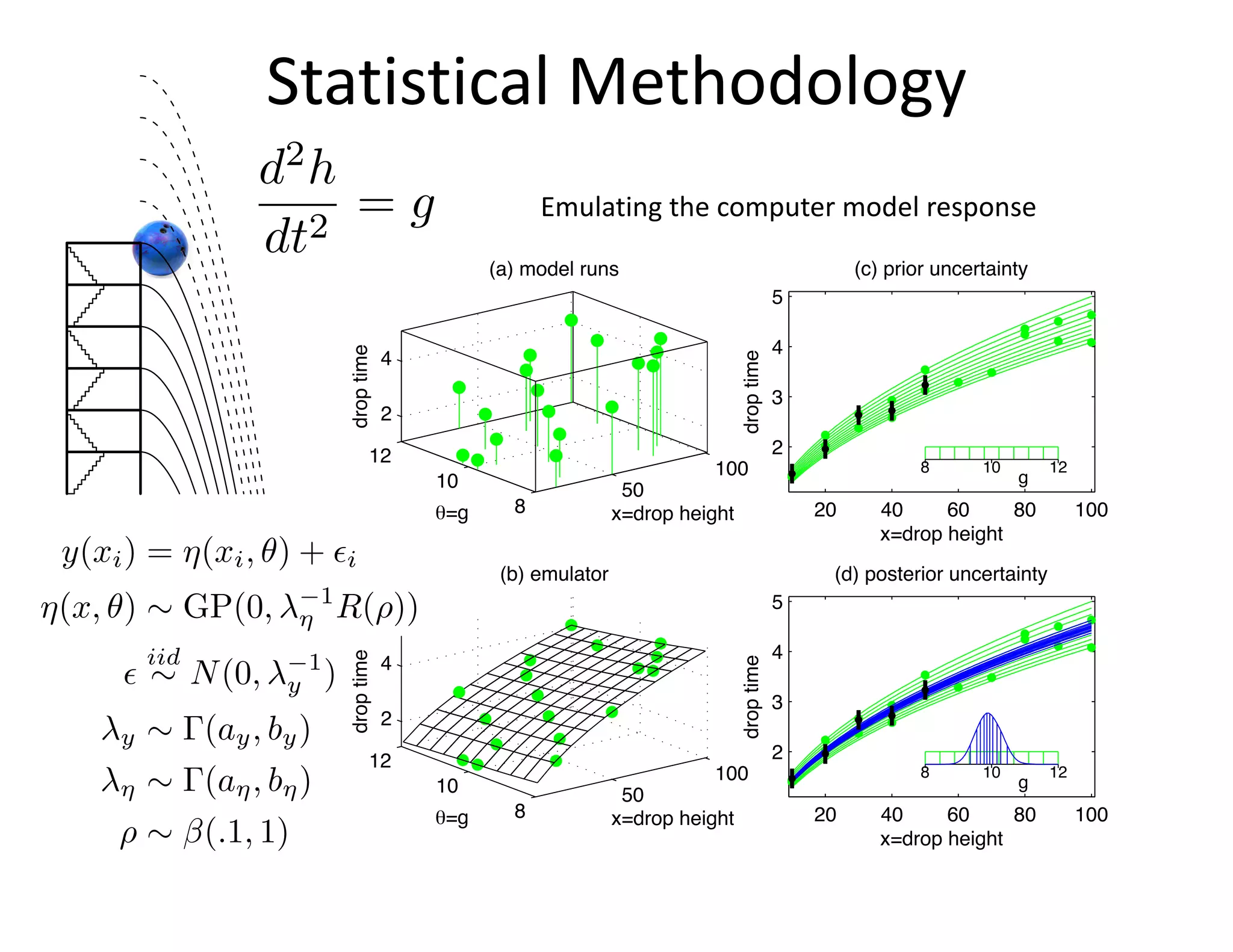
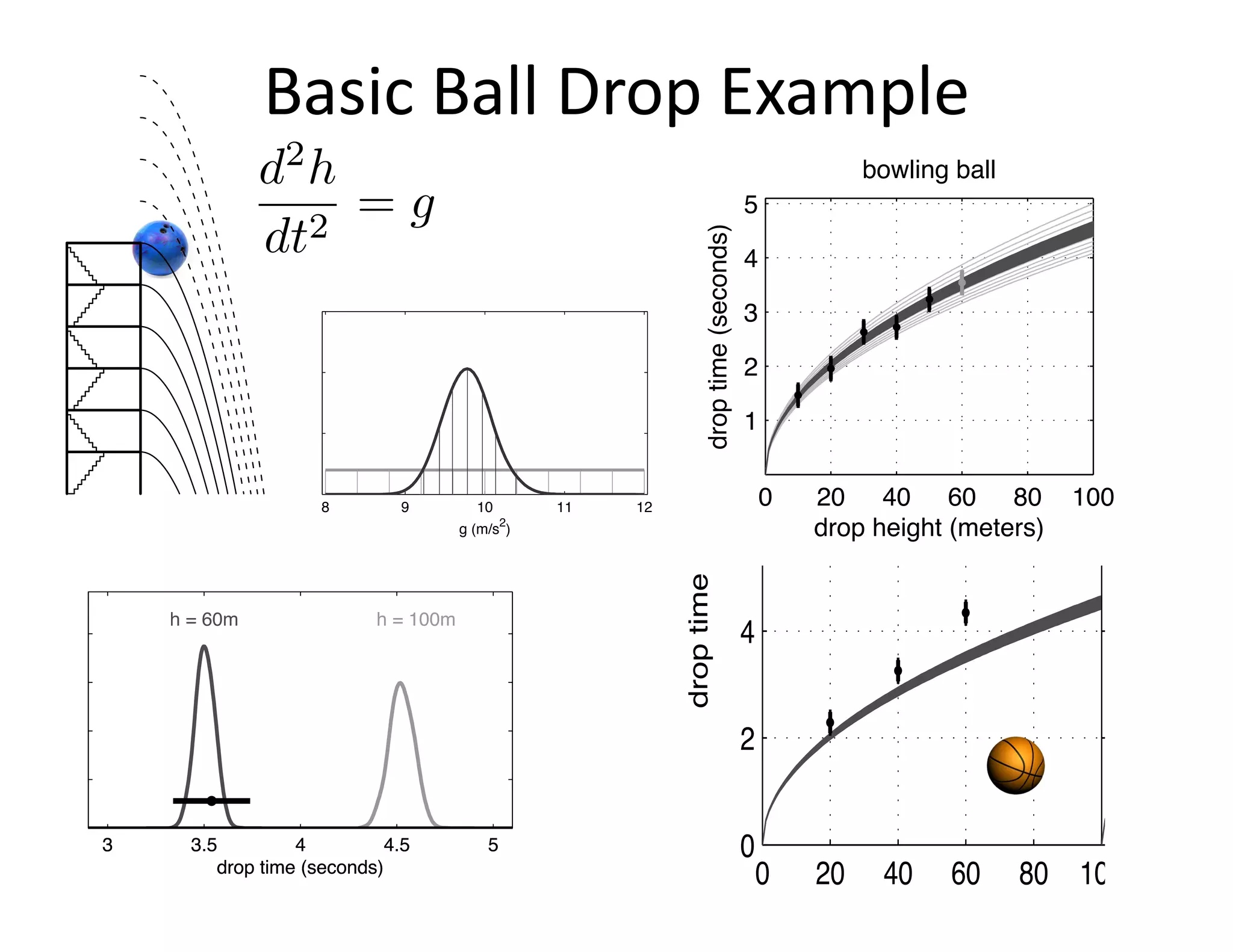
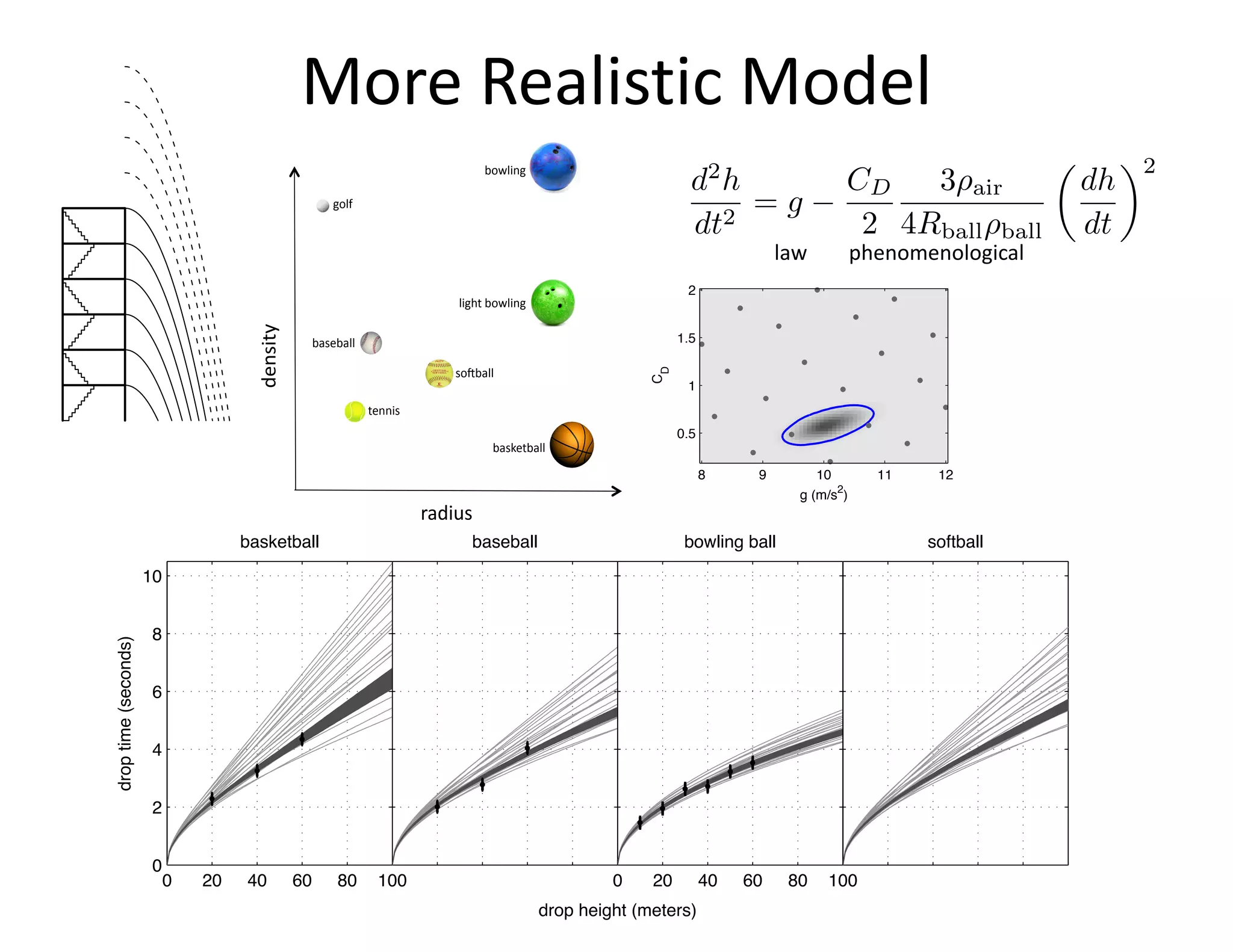
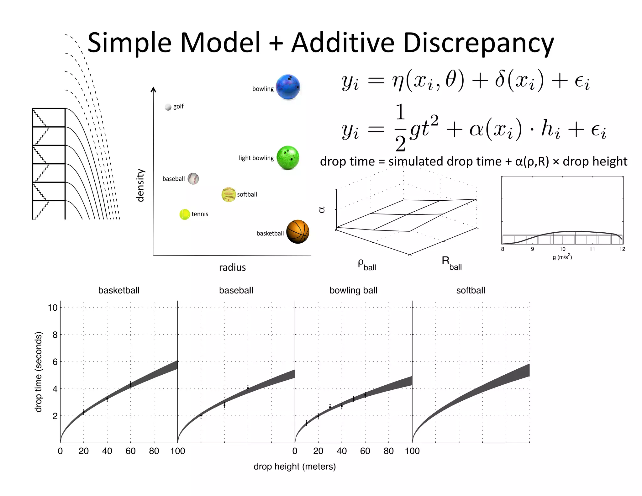
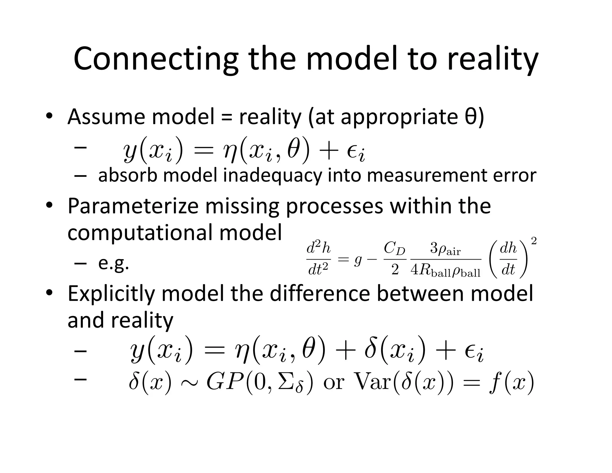


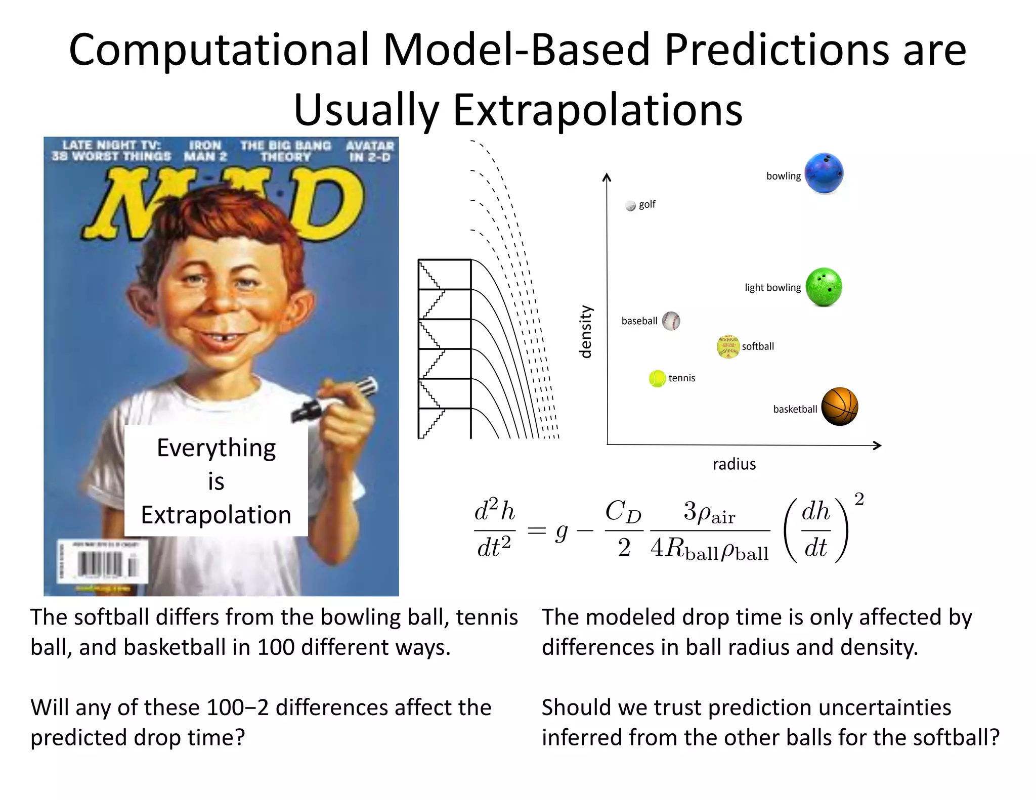
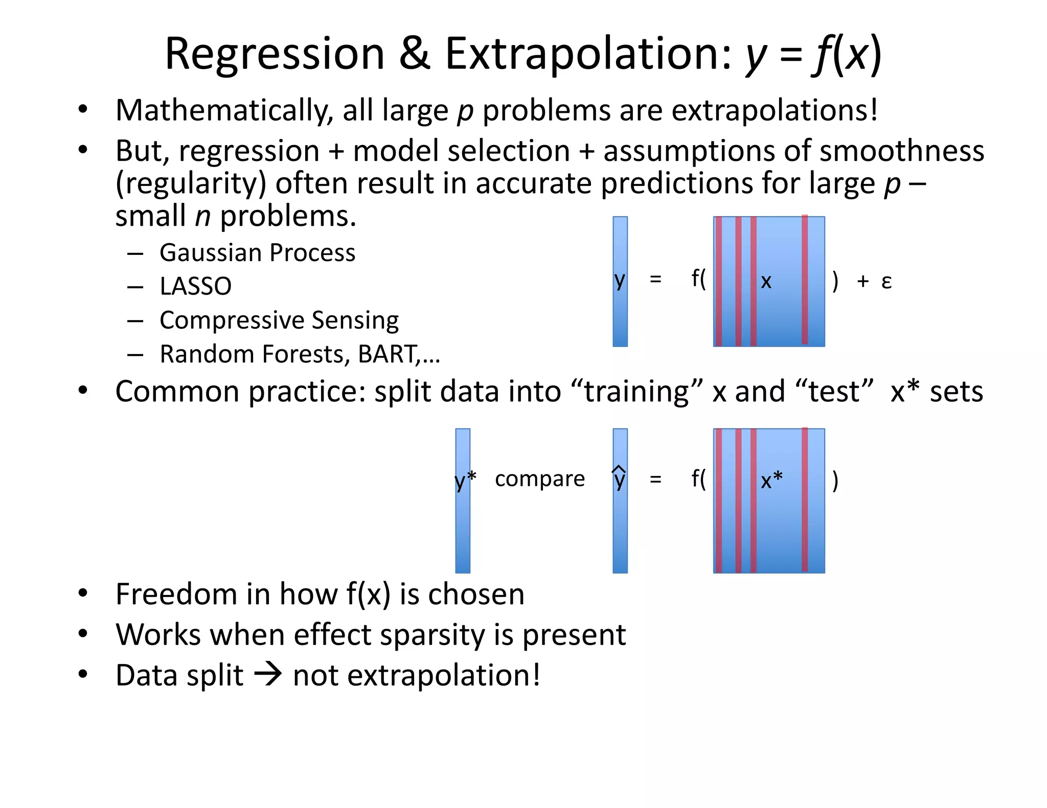
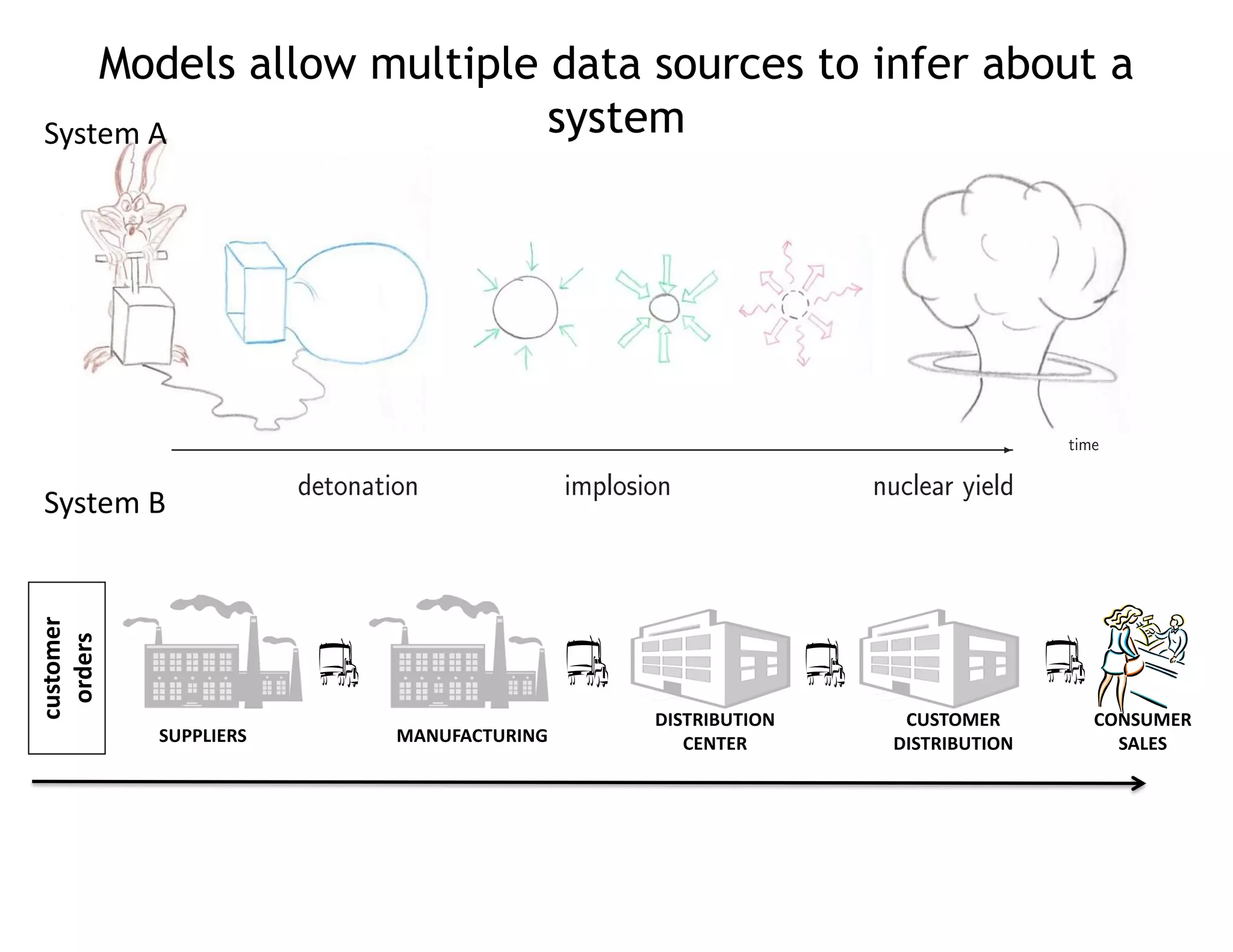


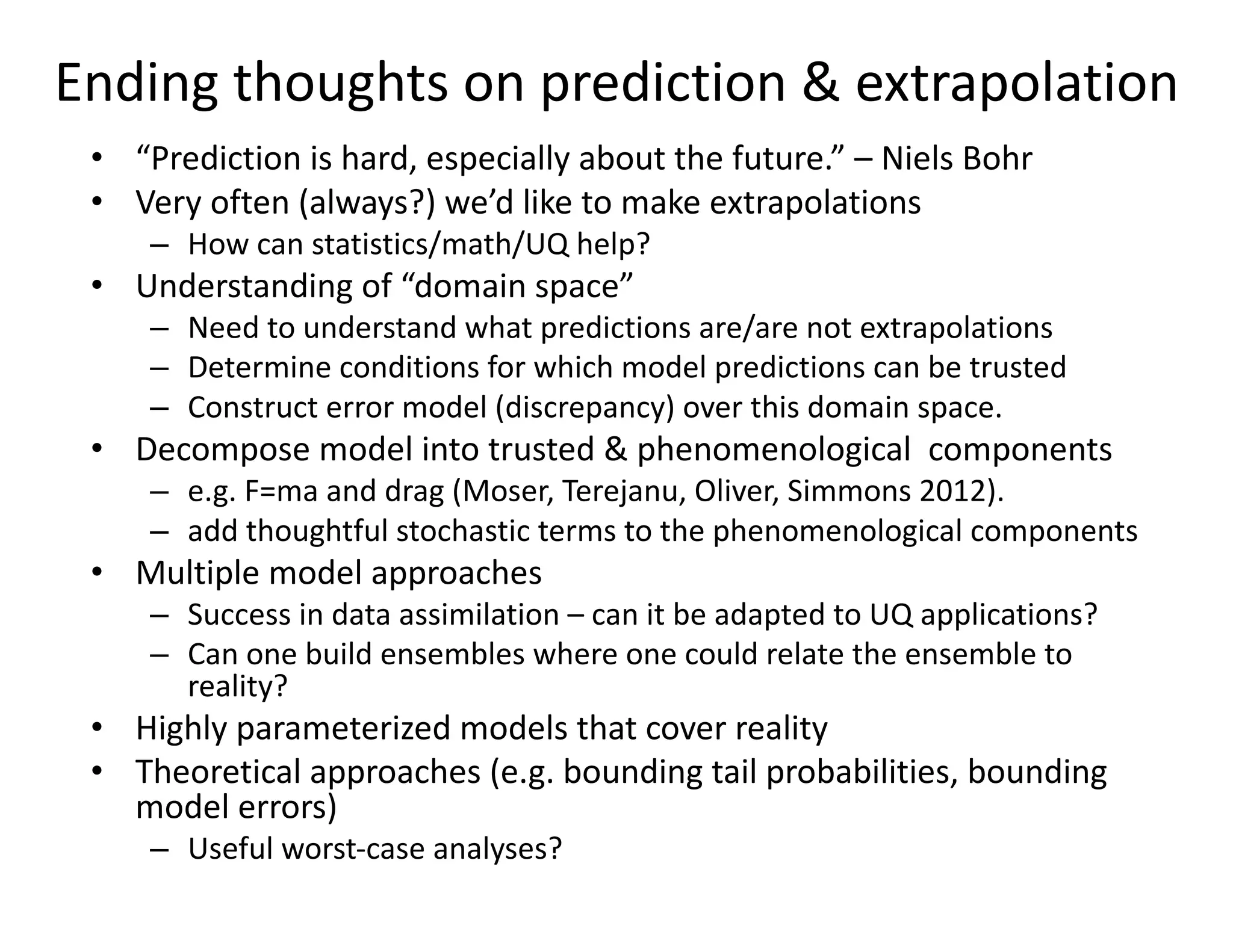
The document discusses methods for quantifying uncertainty in extrapolative predictions using statistical and computational models, focusing on experiments such as dropping balls from heights and radiative shock simulations. It highlights the importance of understanding model limitations and discrepancies when predicting outcomes in extrapolation scenarios. Several examples illustrate the application of these methodologies to improve predictions and manage uncertainties in various experimental settings.