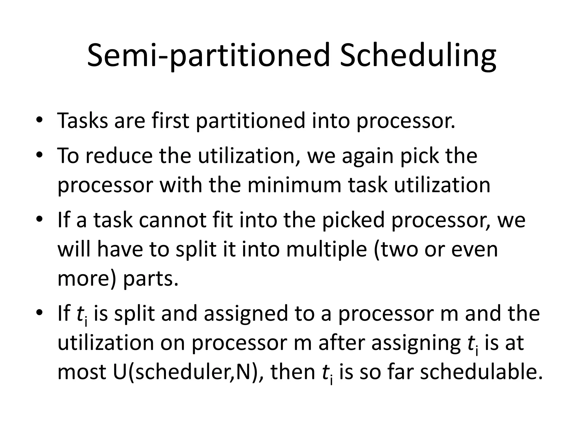
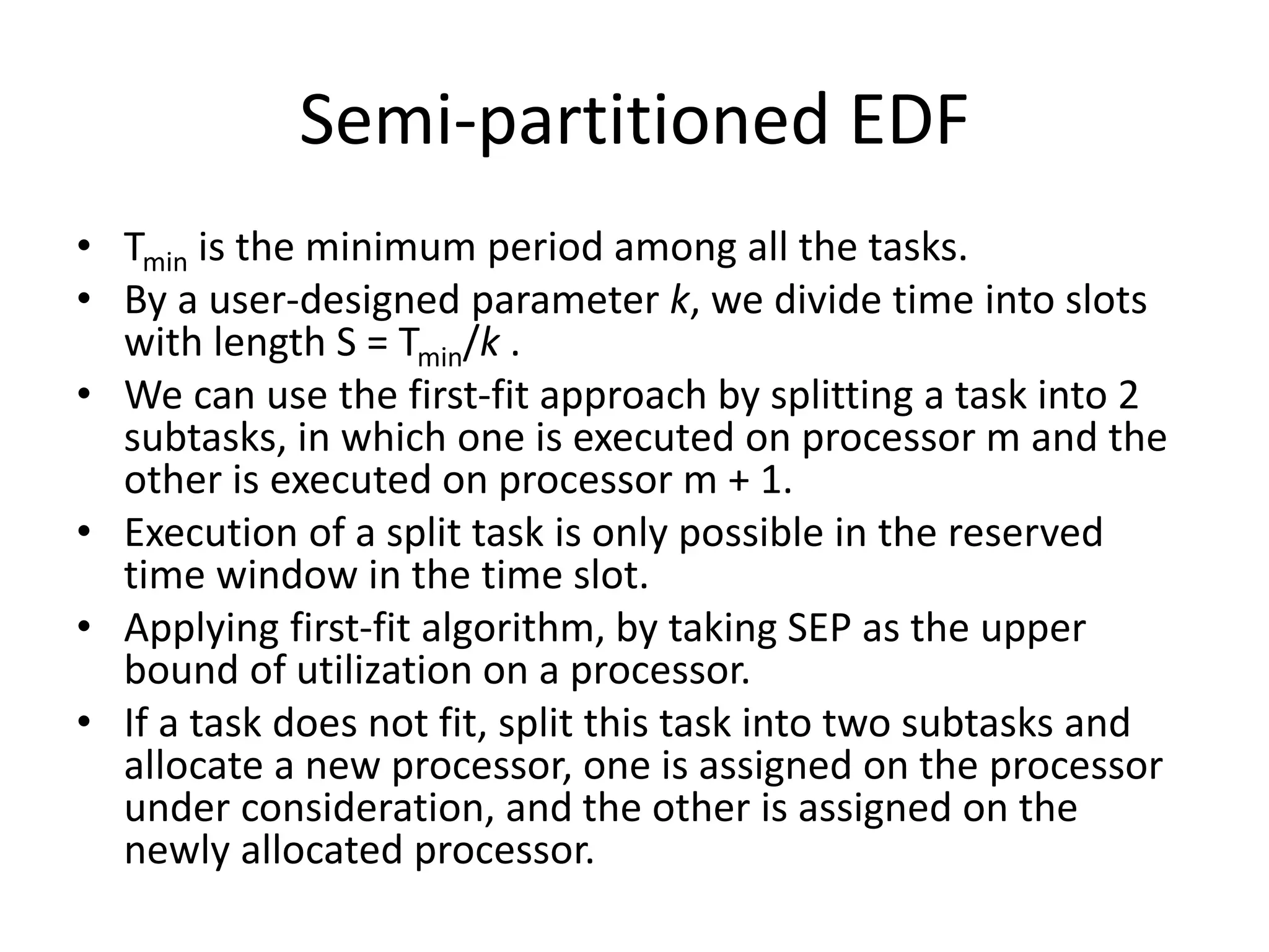
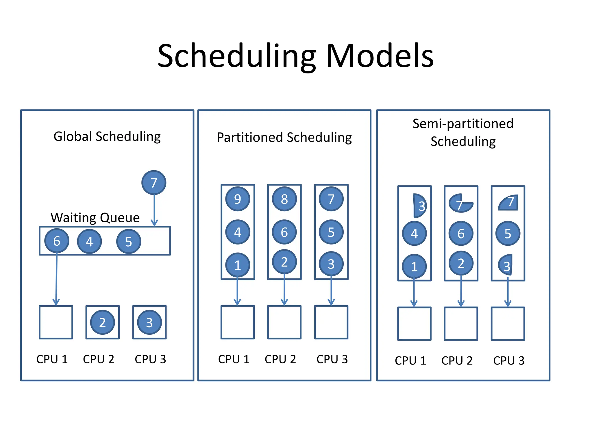
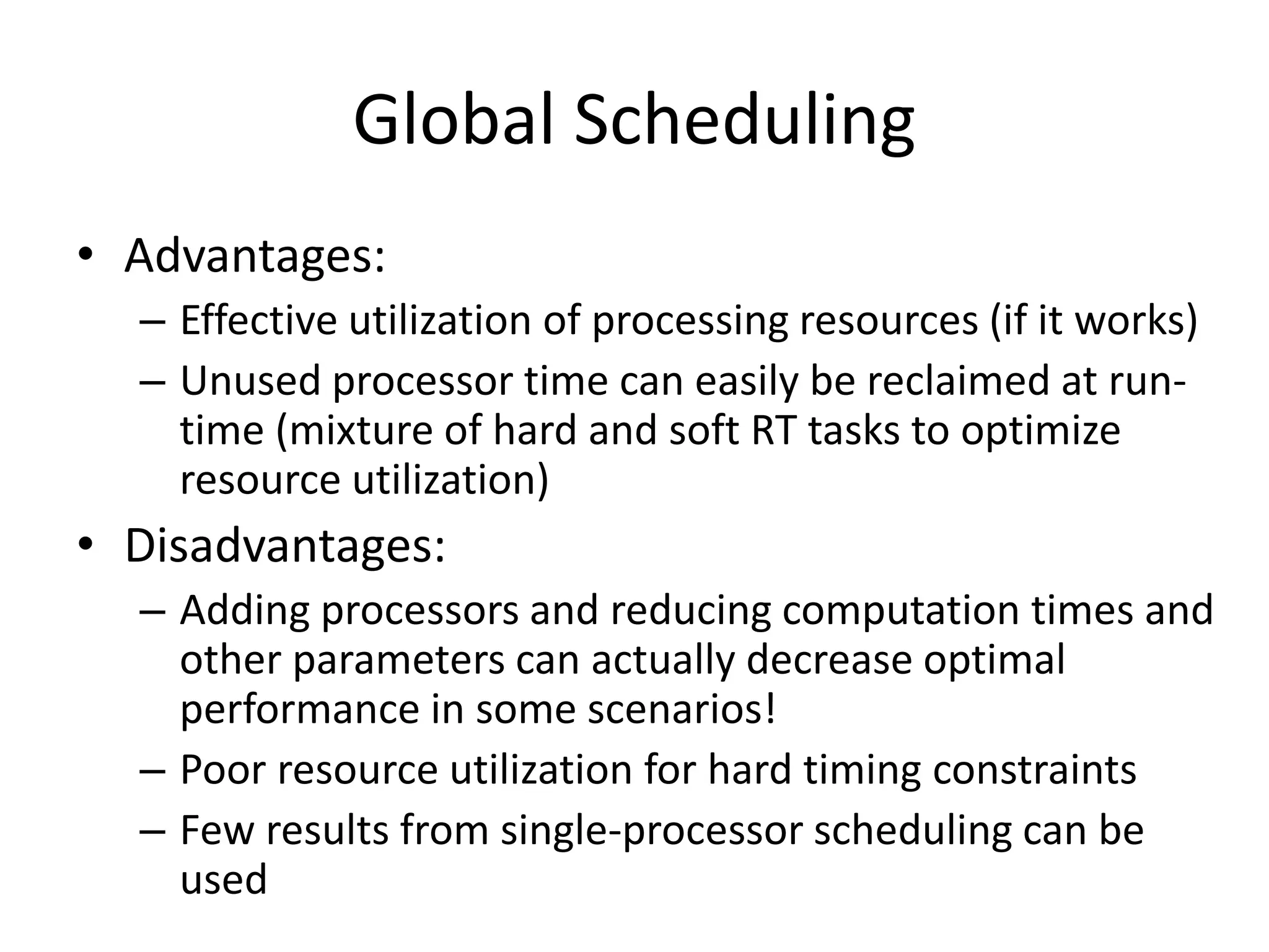
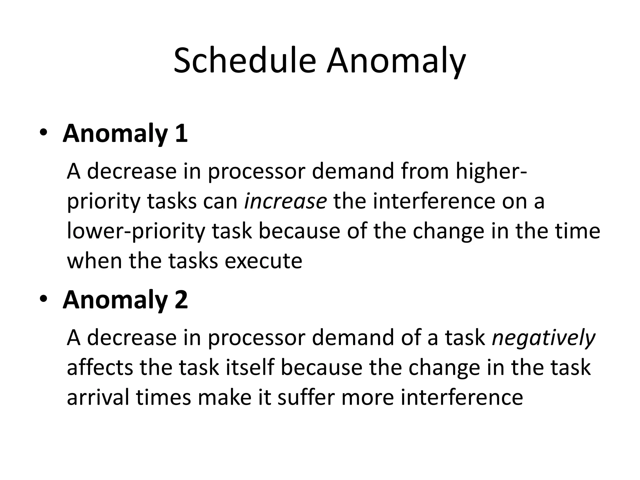
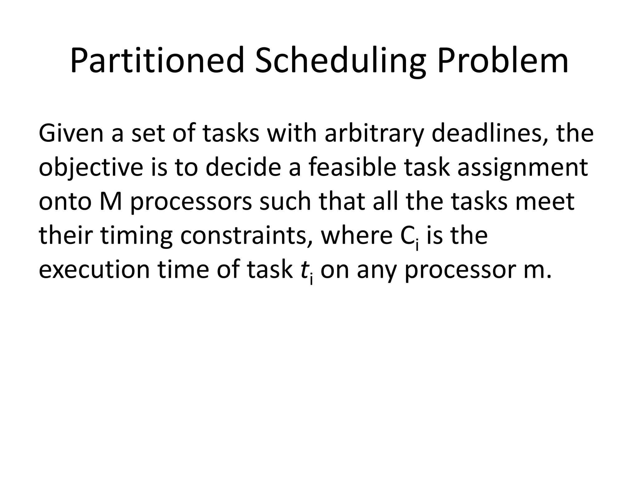
This document discusses different scheduling models for multiprocessor real-time systems, including global scheduling, partitioned scheduling, and semi-partitioned scheduling. Global scheduling uses a shared ready queue and allows tasks to migrate between processors, but can cause overhead from migration and scheduling anomalies. Partitioned scheduling assigns each task to a dedicated processor to avoid migration, but may underutilize processors. Semi-partitioned scheduling first partitions tasks then allows some to migrate to improve utilization.

1. Multiprocessor
Real-Time Scheduling
Embedded System Software Design
Use under the permission of Prof. Ya-
Shu Chen (NTUST)

2. Outline
• Multiprocessor Real-Time Scheduling
• Global Scheduling
• Partitioned Scheduling
• Semi-partitioned Scheduling

3. Multiprocessor Models
• Identical (Homogeneous): All the processors have the same
characteristics, i.e., the execution time of a job is
independent on the processor it is executed.
• Uniform: Each processor has its own speed, i.e., the
execution time of a job on a processor is proportional to the
speed of the processor.
– A faster processor always executes a job faster than slow
processors do.
– For example, multiprocessors with the same instruction set but
with different supply voltages/frequencies.
• Unrelated (Heterogeneous): Each job has its own execution
time on a specified processor
– A job might be executed faster on a processor, but other jobs
might be slower on that processor.
– For example, multiprocessors with different instruction sets.

4. Scheduling Models
• Global Scheduling:
– A job may execute on any processor.
– The system maintains a global ready queue.
– Execute the M highest-priority jobs in the ready queue, where M
is the number of processors.
– It requires high on-line overhead.
• Partitioned Scheduling:
– Each task is assigned on a dedicated processor.
– Schedulability is done individually on each processor.
– It requires no additional on-line overhead.
• Semi-partitioned Scheduling:
– Adopt task partitioning first and reserve time slots (bandwidths)
for tasks that allow migration.
– It requires some on-line overhead.

5. Scheduling Models
6
2 3
4
7
5
CPU 1 CPU 2 CPU 3
Waiting Queue
CPU 1 CPU 2 CPU 3
1
4
9 8
6
2 3
5
7
Global Scheduling
CPU 1 CPU 2 CPU 3
1
4 6
2
5
Partitioned Scheduling
Semi-partitioned
Scheduling
3
3 7 7

6. Global Scheduling
• All ready tasks are kept in a global queue
• A job can be migrated to any processor.
• Priority-based global scheduling:
– Among the jobs in the global queue, the M highest priority
jobs are chosen to be executed on M processors.
– Task migration here is assumed with no overhead.
• Global-EDF: When a job finishes or arrives to the global
queue, the M jobs in the queue with the shortest
absolute deadlines are chosen to be executed on M
processors.
• Global-RM: When a job finishes or arrives to the global
queue, the M jobs in the queue with the highest
priorities are chosen to be executed on M processors.

7. Global Scheduling
• Advantages:
– Effective utilization of processing resources (if it works)
– Unused processor time can easily be reclaimed at run-
time (mixture of hard and soft RT tasks to optimize
resource utilization)
• Disadvantages:
– Adding processors and reducing computation times and
other parameters can actually decrease optimal
performance in some scenarios!
– Poor resource utilization for hard timing constraints
– Few results from single-processor scheduling can be
used

8. Schedule Anomaly
• Anomaly 1
A decrease in processor demand from higher-
priority tasks can increase the interference on a
lower-priority task because of the change in the time
when the tasks execute
• Anomaly 2
A decrease in processor demand of a task negatively
affects the task itself because the change in the task
arrival times make it suffer more interference

9. Anomaly 1

10. Anomaly 2

11. Dhall effect
• Dhall effect : For Global-EDF or Global-RM, the least
upper bound for schedulability analysis is at most 1.
• On 2 processors:
• T3 is not schedulable
Task T D C U
T1 10 10 5 0.5
T2 10 10 5 0.5
T3 12 12 8 0.67

12. Schedulability Test
• A set of periodic tasks t1, t2, . . . , tN with
implicit deadlines is schedulable on M
processors by using preemptive Global EDF
scheduling if
where tk is the task with the largest utilization
Ck/Tk

13. Weakness of Global Scheduling
• Migration overhead
• Schedule Anomaly

14. Partitioned Scheduling
• Two steps:
– Determine a mapping of tasks to processors
– Perform run-time single-processor scheduling
•Partitioned with EDF
– Assign tasks to the processors such that no
processor’s capacity is exceeded (utilization
bounded by 1.0)
– Schedule each processor using EDF

15. Bin-packing Problem
The problem is NP-complete !!

16. Bin-packing to
Multiprocessor Scheduling
• The problem concerns packing objects of
varying sizes in boxes (”bins”) with the
objective of minimizing number of used boxes.
– Solutions (Heuristics): First Fit
• Application to multiprocessor systems:
– Bins are represented by processors and objects by
tasks.
– The decision whether a processor is ”full” or not is
derived from a utilization-based schedulability test.

17. Partitioned Scheduling
• Advantages:
– Most techniques for single-processor scheduling
are also applicable here
• Partitioning of tasks can be automated
– Solving a bin-packing algorithm
• Disadvantages:
– Cannot exploit/share all unused processor time
– May have very low utilization, bounded by 50%

18. Partitioned Scheduling Problem
Given a set of tasks with arbitrary deadlines, the
objective is to decide a feasible task assignment
onto M processors such that all the tasks meet
their timing constraints, where Ci is the
execution time of task ti on any processor m.

19. Partitioned Algorithm
• First-Fit: choose the one with the smallest
index
• Best-Fit: choose the one with the maximal
utilization
• Worst-Fit: choose the one with the minimal
utilization

20. Partitioned Example
• 0.2 -> 0.6 -> 0.4 -> 0.7 -> 0.1 -> 0.3
0.2
0.4
0.6
0.1
0.3
0.7
0.2
0.4
0.6
0.1 0.3
0.7
0.2
0.7
0.1
0.3
0.4
First Fit Best Fit Worst Fit
0.6

21. EDF with First Fit

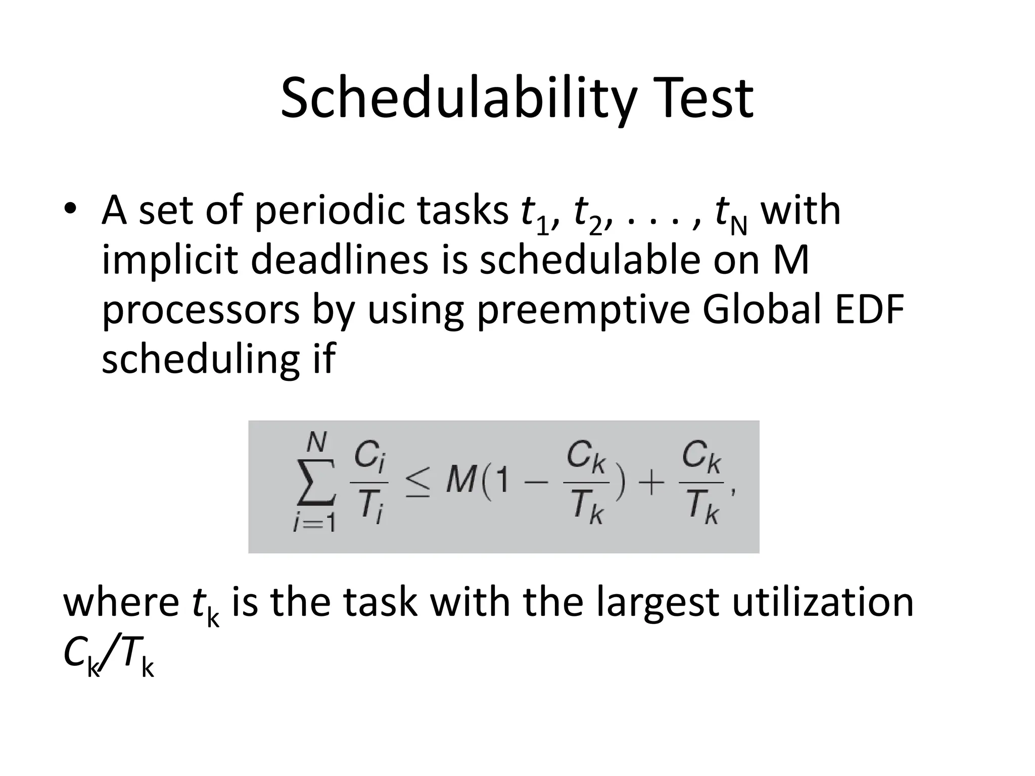
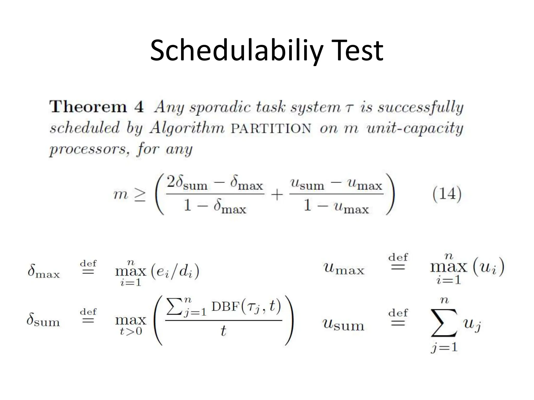
22. Schedulability Test
Lopez [3] proves that the worst-case achievable utilization for
EDF scheduling and FF allocation (EDF-FF) takes the value
If all the tasks have an utilization factor C/T under a value α, where
m is the number of processors
where
1
( , )
1
EDF FF
wc
m
U m



 

 1/
 
  
 

23. Demand Bound Function
• Define demand bound function as
• We need approximation to enforce polynomial-time
schedulability test

24. Deadline Monotonic Partition

25. Schedulabiliy Test

26. Weakness of Partitioned Scheduling
• Restricting a task on a processor reduces the
schedulability
• Restricting a task on a processor makes the
problem NP-hard
• Example: Suppose that there are M processors
and M + 1 tasks with the same period T and
the (worst-case) execution times of all these
M + 1 tasks are T/2 + e with e > 0
– With partitioned scheduling, it is not schedulable

27. Semi-partitioned Scheduling
• Tasks are first partitioned into processor.
• To reduce the utilization, we again pick the
processor with the minimum task utilization
• If a task cannot fit into the picked processor, we
will have to split it into multiple (two or even
more) parts.
• If ti is split and assigned to a processor m and the
utilization on processor m after assigning ti is at
most U(scheduler,N), then ti is so far schedulable.

28. Semi-partitioned EDF
• Tmin is the minimum period among all the tasks.
• By a user-designed parameter k, we divide time into slots
with length S = Tmin/k .
• We can use the first-fit approach by splitting a task into 2
subtasks, in which one is executed on processor m and the
other is executed on processor m + 1.
• Execution of a split task is only possible in the reserved
time window in the time slot.
• Applying first-fit algorithm, by taking SEP as the upper
bound of utilization on a processor.
• If a task does not fit, split this task into two subtasks and
allocate a new processor, one is assigned on the processor
under consideration, and the other is assigned on the
newly allocated processor.

30. Semi-partitioned EDF
• For each time slot, we will reserve two parts.
If a task ti is split, the task can
be served only within these two
pre-defined time slots with length
xi and yi .
A processor can host two split
tasks, ti and tj. ti is served at
the beginning of the time slot,
and tj is served at the end.
The schedule is EDF, but if a split task instance is in the ready queue, it is
executed in the reserved time region.

31. Semi-partitioned EDF
• We can assign all the tasks ti with Ui > SEP on a dedicated
processor. So, we only consider tasks with Ui no larger SEP.
When executing, the reservation to serve ti is to set
xi to S X (f + lo_split(ti )) and yi to S X (f + high_split(ti )).
SEP is set as a constant.

32. Two Split Tasks on a Processor
• For split tasks to be schedulable, the following sufficient
conditions have to be satisfied
– lo_split(ti ) + f + high_split(ti ) + f <= 1 for any split task ti .
– lo_split(tj ) + f + high_split(ti ) + f <= 1 when ti and tj are assigned on
the same processor.
• Therefore, the “magic value” SEP
• However, we still have to guarantee the schedulability of the
non-split tasks. It can be shown that the sufficient condition is

33. Schedulability Test

34. Magic Values: f

35. Magic Values: SEP

36. Reference
• Multiprocessor Real-Time Scheduling
– Dr. Jian-Jia Chen: Multiprocessor Scheduling. Karlsruhe Institute
of Technology (KIT): 2011-2012
• Global Scheduling
– Sanjoy K. Baruah: Techniques for Multiprocessor Global
Schedulability Analysis. RTSS 2007: 119-128
• Partitioned Scheduling
– Sanjoy K. Baruah, Nathan Fisher: The Partitioned Multiprocessor
Scheduling of Sporadic Task Systems. RTSS 2005: 321-329
• Semi-partitioned Scheduling
– Björn Andersson, Konstantinos Bletsas: Sporadic Multiprocessor
Scheduling with Few Preemptions. ECRTS 2008: 243-252

37. See You Next Week

38. Critical Instants?
• The analysis for uniprocessor scheduling is
based on the gold critical instant theorem.
• Synchronous release of events does not lead
to the critical instant for global multiprocessor
scheduling