Download to read offline
![International Journal of Computer Science and Engineering Survey (IJCSES) Vol.11, No.3, Feb
2021
for Implementation of Logic Gates
Santosh Giri and Basanta Joshi
Department of Electronics & Computer Engineering, Institute of
Engineering, Pulchowk Campus, Tribhuvan University.
Lalitpur, Nepal
Abstract. ANN is a computational model that is composed of several processing elements (neu-
rons) that tries to solve a specific problem. Like the human brain, it provides the ability to learn
from experiences without being explicitly programmed. This article is based on the implementa-
tion of artificial neural networks for logic gates. At first, the 3 layers Artificial Neural Network is
designed with 2 input neurons, 2 hidden neurons & 1 output neuron. after that model is trained
by using a backpropagation algorithm until the model satisfies the predefined error criteria (e)
which set 0.01 in this experiment. The learning rate (α) used for this experiment was 0.01. The
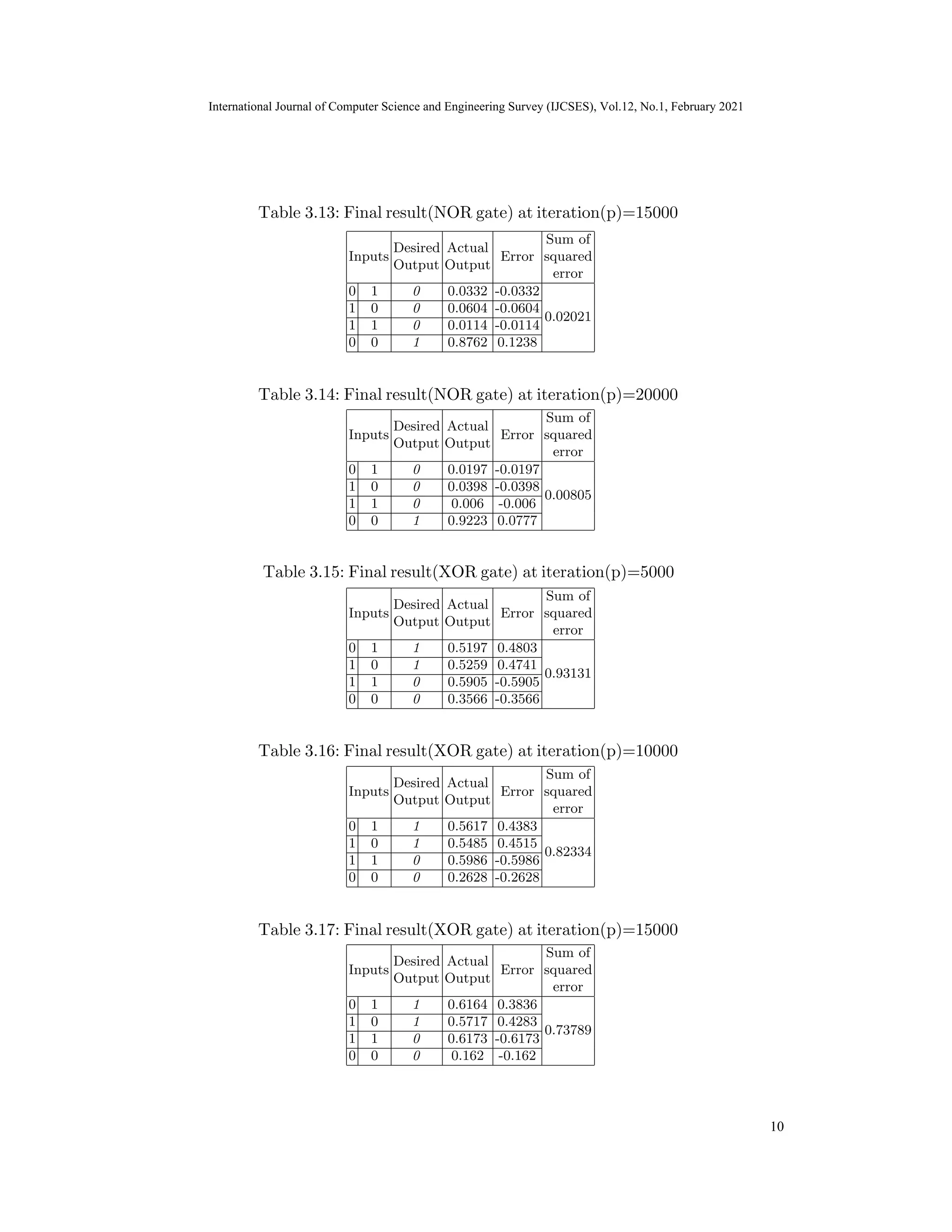
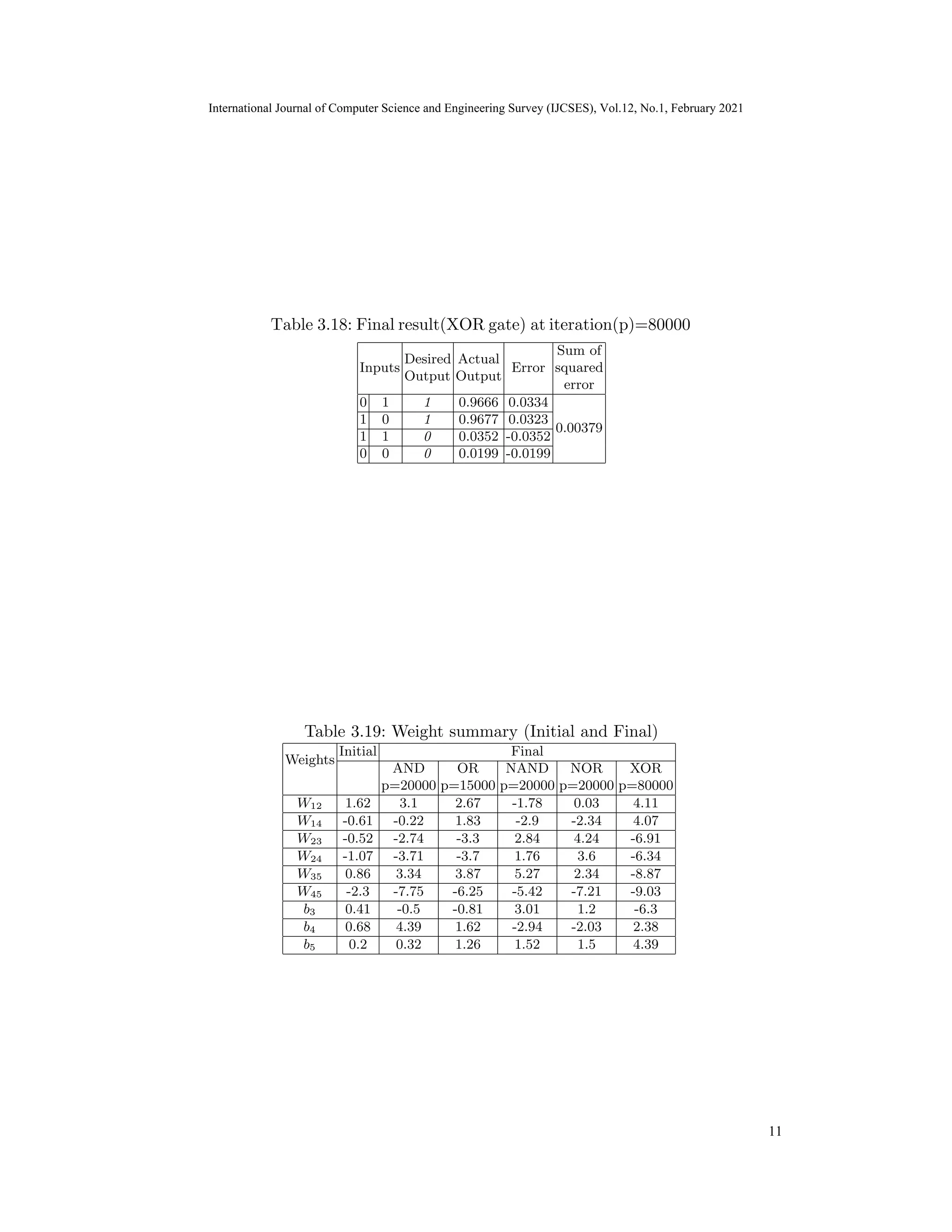
NN model produces correct output at iteration (p)= 20000 for AND, NAND & NOR gate. For
OR & XOR the correct output is predicted at iteration (p)=15000 & 80000 respectively.
1 Introduction
Machine Learning algorithms automatically build a mathematical model using sam-
ple data also known as ’training data’ to make decisions without being specifically
programmed to make those decisions.Machine learning is applicable to fields such
as Speech recognition[7], text prediction[1], handwritten generation[8], genetic al-
gorithms[4], artificial neural networks, natural language processing[6].
1.1 Artificial Neural Network
Artificial neural networks are systems motivated by the distributed, massively par-
allel computation in the brain that enables it to be so successful at complex control
and classification tasks. The biological neural network that accomplishes this can
be mathematically modeled by a weighted, directed graph of highly interconnected
nodes (neurons)[3]. An ANN initially goes through a training phase where it learns
to recognize patterns in data, whether visually, aurally, or textually. During this
training phase, the network compares its actual output produced with what it was
meant to produce the desired output. The difference between both outcomes is
DOI: null 7
International Journal of Computer Science and Engineering Survey (IJCSES), Vol.12, No.1, February 2021
1
DOI: 10.5121/ijcses.2021.12101
Multilayer Backpropagation Neural Networks
adjusted using a set of learning rules called back propagation[5]. This means the
network works backward, going from the output unit to the input units to adjust
Keywords: Machine Learning, Artificial Neural Network, Back propagation, Logic Gates.](https://image.slidesharecdn.com/12121ijcses01-210311104003/75/Multilayer-Backpropagation-Neural-Networks-for-Implementation-of-Logic-Gates-1-2048.jpg)
![2021
Fig. 1.1: Architecture of typical ANN
the weight of its connections between the units until the difference between the
actual and desired outcome produces the lowest possible error. The structure of a
typical Artificial Neural Network is given in Fig. 1.1.
Neuron An ANN has hundreds or thousands of processing units called neu-
rons,which are analogous to biological neurons in human brain. neurons intercon-
nected by nodes. These processing units are made up of input and output units.
The input units receive various forms and structures of information based on an
internal weighting system, and the neural network attempts to learn about the
information presented to it[2]. The neuron multiplies each input (x1, x2, ......, xn)
Fig. 1.2: Architecture of single neuron of an ANN
computes a weighted sum of the input signals as:
X =
n
X
i=1
xiwi
8
(1.1)
International Journal of Computer Science and Engineering Survey (IJCSES), Vol.12, No.1, February 2021
2
by the associated weight (w ,w ,......,w ) and then sums up all the results i.e.](https://image.slidesharecdn.com/12121ijcses01-210311104003/75/Multilayer-Backpropagation-Neural-Networks-for-Implementation-of-Logic-Gates-2-2048.jpg)
![International Journal of Computer Science and Engineering Survey (IJCSES) Vol.11, No.3, Feb
2021
Then, the result is then passed through a non-linear function(f) called activation
of a neuron[9], and has a threshold value 0θ0. Then the result is compared with a
threshold value which gives the output as either ‘00 or ‘10. If the weighted sum is
less than 0θ0 then neuron output is ’1’ otherwise 0. In general, the neuron uses step
function (1.2) as activation functions.
Y ={+1,ifX>θ
0,ifX<θ (1.2)
1.2 Back-propagation multilayer neural networks
In the backpropagation neural network, input signals are propagated on a layer-
by-layer basis from input to output layer for forward propagation and output to
input for backward propagation. The hidden layer is stacked in between inputs
and outputs, which allows neural networks to learn more complicated features. The
learning in multi-layer neural networks processed the same way as in perceptron.
At first, a training set of input patterns is presented to the network and then the
network computes its output, if there is a difference between the desired output
and actual output (an error) then the weights are adjusted to reduce the difference.
1.3 Backpropagation Algorithms
To train multi-layer Artificial Neural Network designed here, the backpropagation
algorithm[5] is used. Backpropagation is the set of learning rules used to guide
artificial neural networks. The working mechanism of this algorithm is as follows:
Step 1: Initialization:
Initialization of initial parameters such as weights (W), threshold (θ), learning
rate (α) & bias value (b) and number of iterations (p). Initialize all the initial
parameters inside a small range.
Step 2: Activations:
Activate the networks by applying all sets of possible inputs x1(p), x2(p),
x3(p), ......xn(p) & desired outputs yd1(p), yd2(p), yd3(p), ......, ydn(p).
i. Calculate the actual outputs in hidden layer as:
yj(p) = sigmoid[
n
X
i=1
xi(p) ∗ wij(p) − θj] (1.3)
where,
n = number of inputs of neuron j in hidden layer and Activation function used
here is sigmoid function defined as:
Y sigmoid
=
1
1 + e−X
9
(1.4)
International Journal of Computer Science and Engineering Survey (IJCSES), Vol.12, No.1, February 2021
3
function. An activation function is the function that describes the output behavior](https://image.slidesharecdn.com/12121ijcses01-210311104003/75/Multilayer-Backpropagation-Neural-Networks-for-Implementation-of-Logic-Gates-3-2048.jpg)
![International Journal of Computer Science and Engineering Survey (IJCSES) Vol.11, No.3, Feb
2021
yk(p) = sigmoid[
m
X
j=1
xj(p) ∗ wjk(p)−k] (1.5)
Where,
m = number of inputs of neuron k in output layer.
Step 3: Error gradient and weights:
Calculate the error gradient and update the weights by propagating backward
through the networks.
i. Calculate the error gradient δ for neurons in output layer:
δk(p) = yk(p) ∗ [1 − yk(p)] ∗ ek(p) (1.6)
Where, ek(p) = yd,k(p) − yk(p)
ii. Calculate the weight corrections as:
5wjk(p) = α ∗ yj(p) ∗ δk(p) (1.7)
iii. Update the weights of neurons at output layer as:
wjk(p + 1) = wjk(p) + 5wjk(p) (1.8)
iv. Calculate the error gradient δ for neurons in hidden layer:
δj(p) = yj(p) ∗ [1 − yj(p)] ∗
l
X
k=1
δk(p) ∗ wjk(p) (1.9)
v. Calculate the weight corrections as:
5wij(p) = α ∗ xi(p) ∗ δj(p) (1.10)
vi. Update the weights of neurons at hidden layer as:
wij(p + 1) = wij(p) + 5wij(p) (1.11)
Step 4:
until predefined error criteria is fulfilled.
10
International Journal of Computer Science and Engineering Survey (IJCSES), Vol.12, No.1, February 2021
4
ii. Calculate theactual outputin outputlayer as:
Increase the value of p(iteration) by 1, go to Step 2 and repeat this process](https://image.slidesharecdn.com/12121ijcses01-210311104003/75/Multilayer-Backpropagation-Neural-Networks-for-Implementation-of-Logic-Gates-4-2048.jpg)
![International Journal of Computer Science and Engineering Survey (IJCSES) Vol.11, No.3, Feb
2021
In this article, we have used a multilayer neural network with two input neurons,
two hidden neurons, and one output neurons as shown in Fig. 2.1. We are doing so
because all the logic gates: AND, OR, NAND, NOR, and XOR being implemented
here have two inputs signals and one output signals with signal values being either
’1’ or ’0’. Here W13, W14, W23, W24 are weights associated between neurons of
input layer & hidden layer and W35, W45 are weights associated between hidden
layer and output layer. biases: b3, b4 & b5 are values associated with each node in
the intermediate (hidden) and output layers of the network, are treated in the same
manner as other weights.
Fig. 2.1: Multi-layer back-propagation neural networks with two input neurons and
single output neuron
2.2 Implementation of multi-layer neural networks.
To train the multi-layer neural network designed here we have used the back-
propagation algorithm[5] describes in section(1.3). The training of the NN model
takes place in two steps. In the first step of training, input signals were presented
to the input layer of the network. Then network propagates the signals from layer
to layer until the output is generated by the output layer. If the output is differ-
ent from the desired output then an error is calculated and propagated backward
from the output layer to the input layer and the weights are modified accordingly.
11
2 Methodology
International Journal of Computer Science and Engineering Survey (IJCSES), Vol.12, No.1, February 2021
5
2.1 Designing a Backpropagation multilayer neural network
This process is repeated until a predefined criteria (sum of squared error)is fulfilled.](https://image.slidesharecdn.com/12121ijcses01-210311104003/75/Multilayer-Backpropagation-Neural-Networks-for-Implementation-of-Logic-Gates-5-2048.jpg)
![International Journal of Computer Science and Engineering Survey (IJCSES) Vol.11, No.3, Feb
2021
4 Conclusions
In this article, the Multi-layer artificial neural network for logic gates is implemented
here satisfies error criteria (0.01) at learning rate(α=0.01), iterations(p)=20000 for
logic gates: AND, NAND, NOR and for OR & XOR gate predicted correct output
at p=15000 & p=80000 respectively.
References
[1] Adam Coates et al. “Text detection and character recognition in scene images
with unsupervised feature learning”. In: Document Analysis and Recognition
(ICDAR), 2011 International Conference on. IEEE. 2011, pp. 440–445.
[2] JAKE FRANKENFIELD. Artificial Neural Network. 2020. url: https://
www.investopedia.com/terms/a/artificial-neural-networks-ann.asp
(visited on 07/07/2020).
[3] Mohamad H Hassoun et al. Fundamentals of artificial neural networks. MIT
press, 1995.
[4] John H Holland. “Genetic algorithms”. In: Scientific american 267.1 (1992),
pp. 66–73.
[5] Yann LeCun et al. “Backpropagation applied to handwritten zip code recog-
nition”. In: Neural computation 1.4 (1989), pp. 541–551.
[6] Christopher Manning and Hinrich Schutze. Foundations of statistical natural
language processing. MIT press, 1999.
[7] Dabbala Rajagopal Reddy. “Speech recognition by machine: A review”. In:
Proceedings of the IEEE 64.4 (1976), pp. 501–531.
[8] Tamás Varga, Daniel Kilchhofer, and Horst Bunke. “Template-based synthetic
handwriting generation for the training of recognition systems”. In: Proceed-
ings of the 12th Conference of the International Graphonomics Society. 2005,
pp. 206–211.
[9] Bill Wilson. The Machine Learning Dictionary. 2020. url: http://www.cse.
18
International Journal of Computer Science and Engineering Survey (IJCSES), Vol.12, No.1, February 2021
12
successfully by using the Backpropagation algorithm. The NN model implemented
unsw.edu.au/billw/mldict.html/activnfn (visited on 07/01/2020).](https://image.slidesharecdn.com/12121ijcses01-210311104003/75/Multilayer-Backpropagation-Neural-Networks-for-Implementation-of-Logic-Gates-12-2048.jpg)

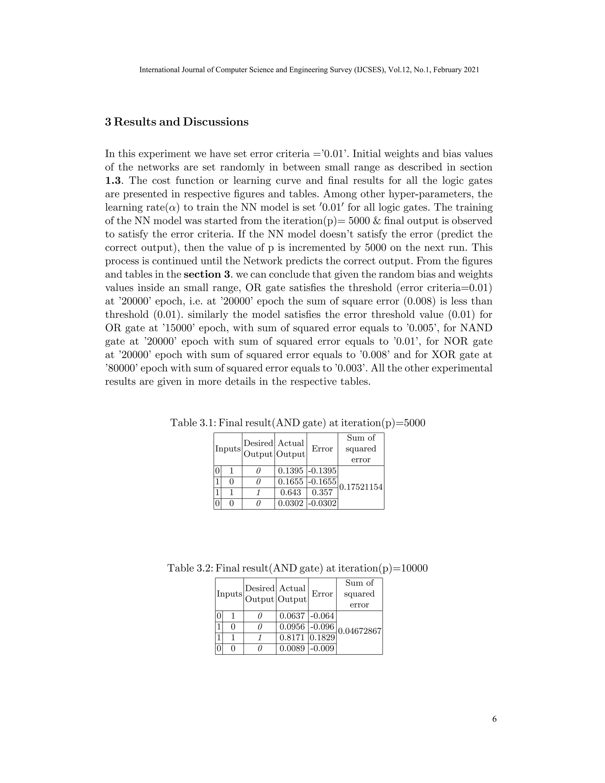
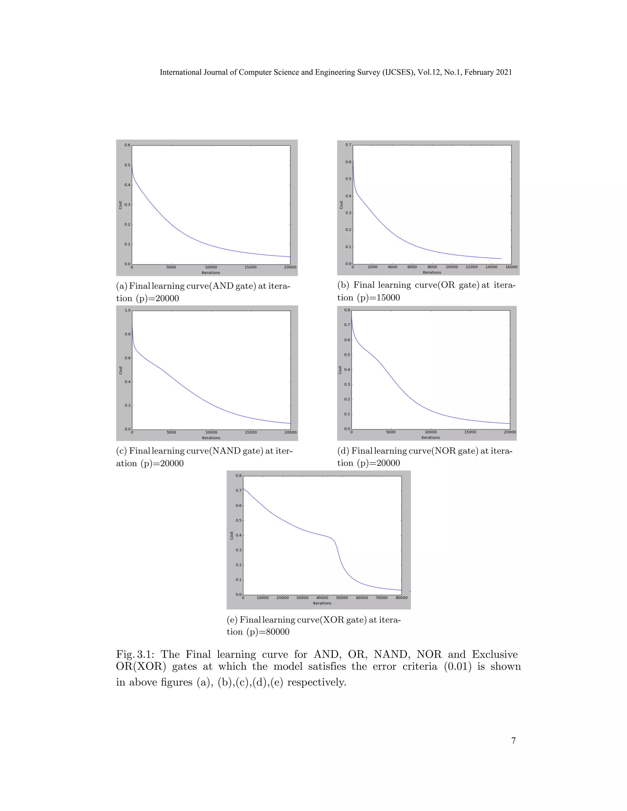
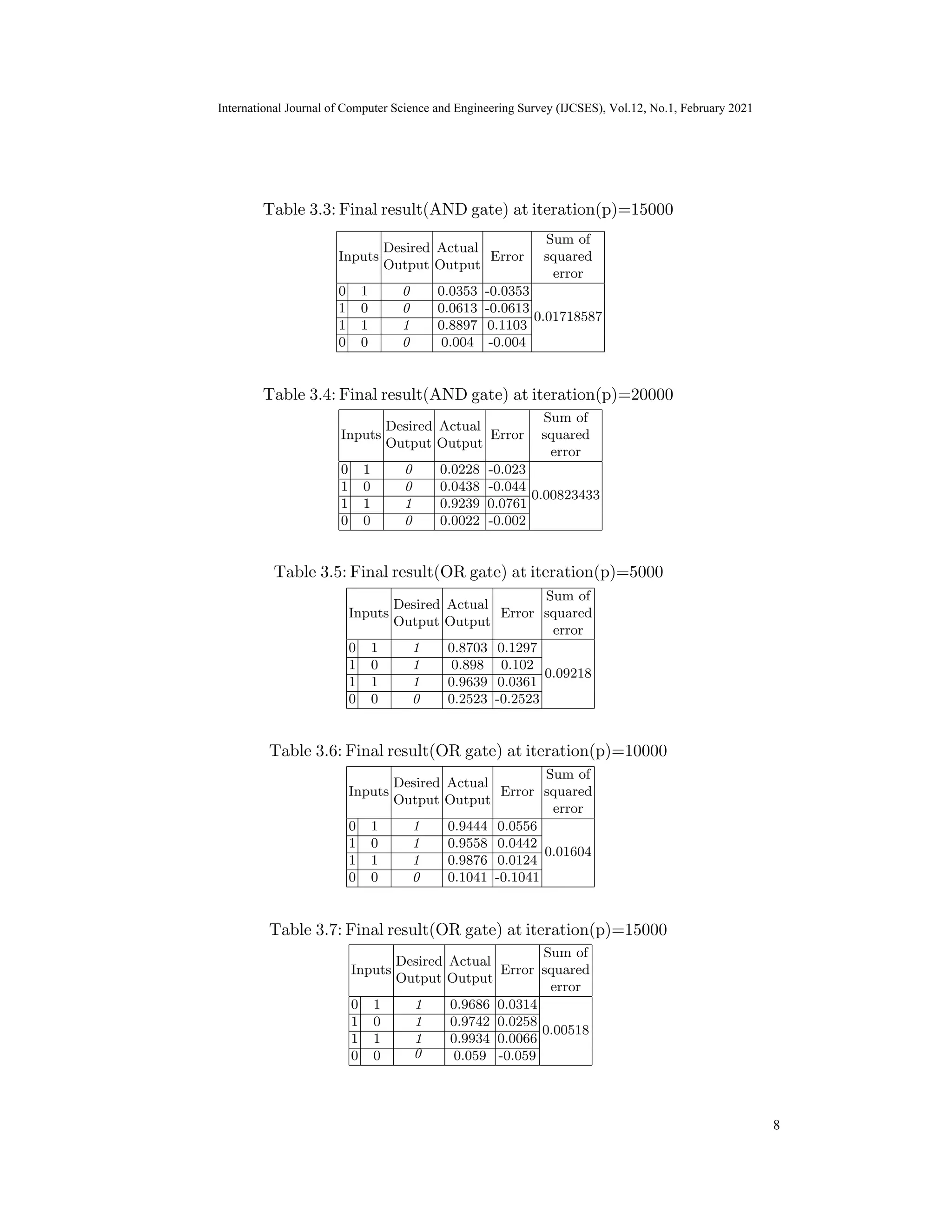
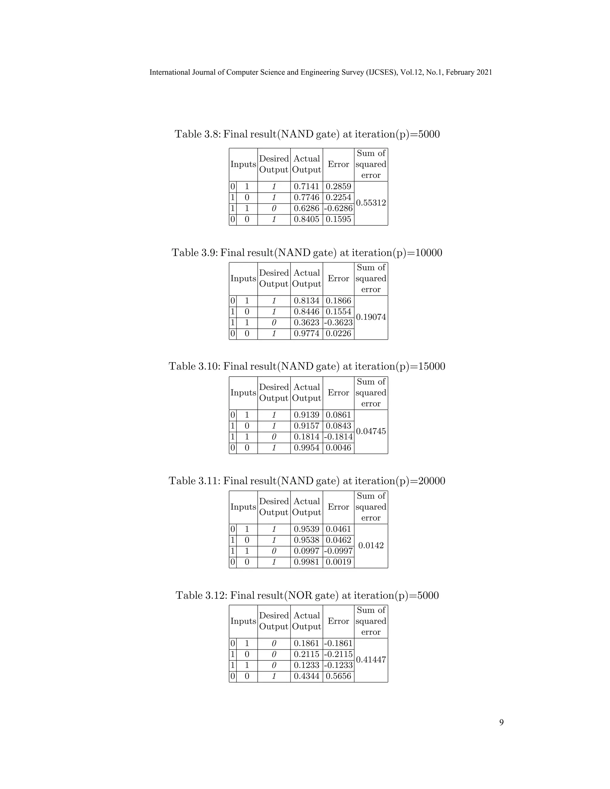
The document discusses the implementation of artificial neural networks (ANNs) to model logic gates using a 3-layer ANN structure with specific configurations for inputs, hidden layers, and outputs. A backpropagation algorithm is utilized for training the network until a predefined error threshold of 0.01 is achieved, with varying iterations required for different gates. Results show that the ANN successfully predicts outputs for various logic gates, demonstrating the effectiveness of ANNs in machine learning applications.