Download as PDF, PPTX
![Bidirectional RNN/LSTM
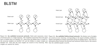
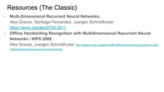
There are many situations when you see the whole sequence at once (OCR,
speech recognition, translation, caption generation, …).
So you can scan the [1-d] sequence in both directions, forward and backward.
Here comes BLSTM (Graves, Schmidhuber, 2005).](https://image.slidesharecdn.com/mdrnn-yandexmoscowcv-160427182305/85/Multidimensional-RNN-18-320.jpg)
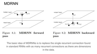
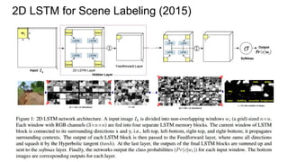
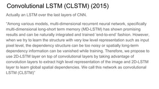
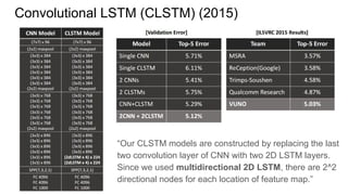
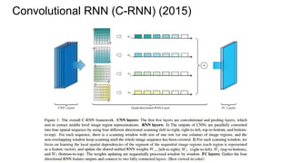
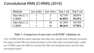
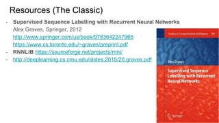
![Convolutional RNN (C-RNN) (2015)
“The C-RNN is trained in an end-to-end manner from raw pixel images. CNN
layers are firstly processed to generate middle level features. RNN layer is then
learned to encode spatial dependencies.”
“In [13], MDLSTM was proposed to solve the handwriting recognition problem by
using RNN. Different from this work, we utilize quad-directional 1D RNN
instead of their 2D RNN, our RNN is simpler and it has fewer parameters, but it
can already cover the context from all directions. Moreover, our C-RNN make both
use of the discriminative representation power of CNN and contextual information
modeling capability of RNN, which is more powerful for solving large scale image
classification problem.”
Funny, it’s not an LSTM. Just simple RNN.](https://image.slidesharecdn.com/mdrnn-yandexmoscowcv-160427182305/85/Multidimensional-RNN-59-320.jpg)
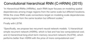
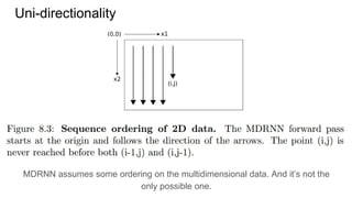
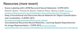
![Convolutional hierarchical RNN (C-HRNN) (2015)
“Thus, inspired by [22], we generate “2D sequences” for images, and each element
simultaneously receives spatial contextual references from its 2D neighborhood
elements.”](https://image.slidesharecdn.com/mdrnn-yandexmoscowcv-160427182305/85/Multidimensional-RNN-65-320.jpg)
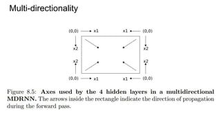
![Example #4:
ReNet (2015)
[Francesco Visin, Kyle Kastner, Kyunghyun Cho, Matteo Matteucci, Aaron Courville, Yoshua Bengio]
http://arxiv.org/abs/1505.00393](https://image.slidesharecdn.com/mdrnn-yandexmoscowcv-160427182305/85/Multidimensional-RNN-68-320.jpg)
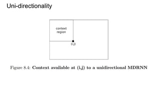
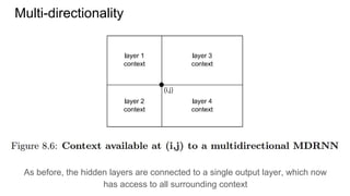
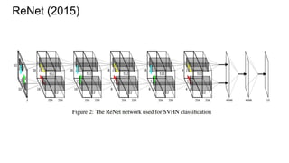
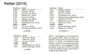
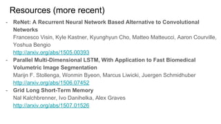
![ReNet (2015)
“Our model relies on purely uni-dimensional RNNs coupled in a novel way, rather
than on a multi-dimensional RNN. The basic idea behind the proposed ReNet
architecture is to replace each convolutional layer (with convolution+pooling
making up a layer) in the CNN with four RNNs that sweep over lower-layer
features in different directions: (1) bottom to top, (2) top to bottom, (3) left to right
and (4) right to left.”
“The main difference between ReNet and the model of Graves and Schmidhuber
[2009] is that we use the usual sequence RNN, instead of the multidimensional
RNN.“](https://image.slidesharecdn.com/mdrnn-yandexmoscowcv-160427182305/85/Multidimensional-RNN-69-320.jpg)
![ReNet (2015)
“One important consequence of the proposed approach
compared to the multidimensional RNN is that the
number of RNNs at each layer scales now linearly with
respect to the number of dimensions d of the input
image (2d). A multidimensional RNN, on the other
hand, requires the exponential number of RNNs at each
layer (2d
). Furthermore, the proposed variant is more
easily parallelizable, as each RNN is dependent only
along a horizontal or vertical sequence of patches. This
architectural distinction results in our model being much
more amenable to distributed computing than that of
Graves and Schmidhuber [2009]”.
… But for d=2 2d == 2d](https://image.slidesharecdn.com/mdrnn-yandexmoscowcv-160427182305/85/Multidimensional-RNN-70-320.jpg)
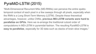
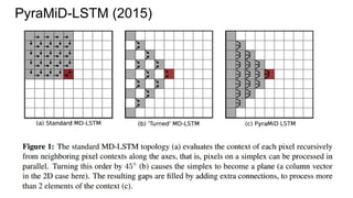
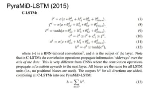
![Example #5: “The Empire Strikes Back”
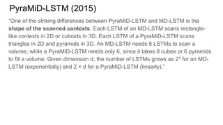
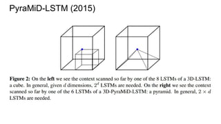
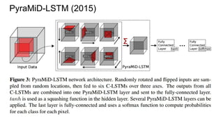
PyraMiD-LSTM (2015)
[Marijn F. Stollenga, Wonmin Byeon, Marcus Liwicki, Juergen Schmidhuber]
http://arxiv.org/abs/1506.07452](https://image.slidesharecdn.com/mdrnn-yandexmoscowcv-160427182305/85/Multidimensional-RNN-73-320.jpg)
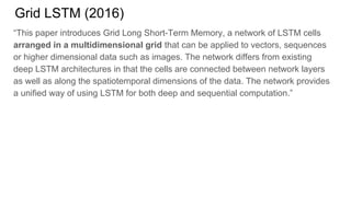
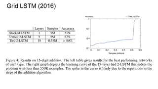
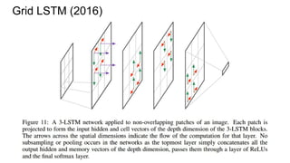
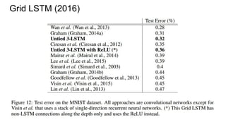
![Example #6: Grid LSTM (ICLR 2016)
(Graves again!)
[Nal Kalchbrenner, Ivo Danihelka, Alex Graves]
http://arxiv.org/abs/1507.01526](https://image.slidesharecdn.com/mdrnn-yandexmoscowcv-160427182305/85/Multidimensional-RNN-83-320.jpg)


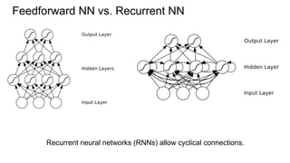
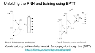
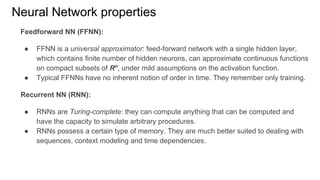
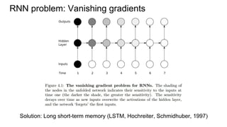
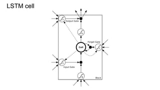
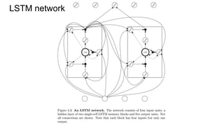
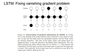
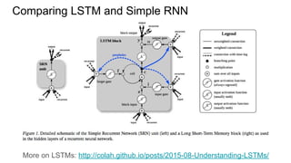
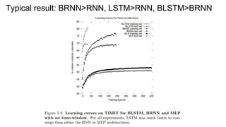
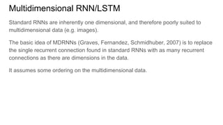
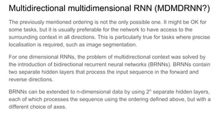
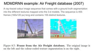
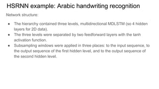
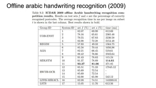
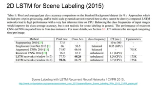
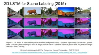
This document provides an overview of multi-dimensional RNNs and some architectural issues and recent results related to them. It begins with an introduction to RNNs compared to feedforward neural networks, and solutions like LSTM and GRU to address the vanishing gradient problem. It then discusses several generalizations of the simple RNN architecture, including directionality with BRNN/BLSTM, dimensionality with MDRNN/MDLSTM, and directionality + dimensionality with MDMDRNN. It also covers hierarchical subsampling with HSRNN. The document concludes by summarizing some recent examples that apply these ideas, such as 2D LSTM for scene labeling, as well as new ideas like ReNet, PyraMiD-LSTM, and Grid LSTM.


![ViT (Vision Transformer) Review [CDM]](https://cdn.slidesharecdn.com/ss_thumbnails/vitreviewcdm-201012184226-thumbnail.jpg?width=640&height=640&fit=bounds)


![[DL輪読会]Real-Time Semantic Stereo Matching](https://cdn.slidesharecdn.com/ss_thumbnails/real-timesemanticstereomatching-sugisakihiroaki-191213003224-thumbnail.jpg?width=640&height=640&fit=bounds)


![[DL Hacks]Semantic Instance Segmentation with a Discriminative Loss Function](https://cdn.slidesharecdn.com/ss_thumbnails/taniai20180528-180528084124-thumbnail.jpg?width=640&height=640&fit=bounds)


![Artificial Intelligence (lecture for schoolchildren) [rus]](https://cdn.slidesharecdn.com/ss_thumbnails/artificialintelligencelectureforschoolchildrenrus-200823192321-thumbnail.jpg?width=640&height=640&fit=bounds)


