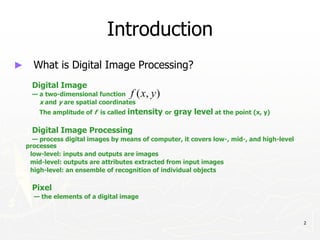
This document provides an introduction to digital image processing. It discusses what digital image processing is, the origins of the field, and sources for digital images like the electromagnetic spectrum. It also covers fundamental steps like image acquisition, representation, sampling and quantization. Key concepts discussed include pixels, pixel relationships, interpolation methods, spatial and intensity resolution, and image representation in MATLAB.


![38
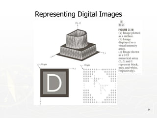
Representing Digital Images
► Discrete intensity interval [0, L-1], L=2k
► The number b of bits required to store a M × N
digitized image
b = M × N × k](https://image.slidesharecdn.com/module1-231113060911-d90f796e/85/Module-1-pptx-38-320.jpg)


![74
Distance Measures
► Given pixels p, q and z with coordinates (x, y), (s, t),
(u, v) respectively, the distance function D has
following properties:
a. D(p, q) ≥ 0 [D(p, q) = 0, iff p = q]
a. D(p, q) = D(q, p)
a. D(p, z) ≤ D(p, q) + D(q, z)](https://image.slidesharecdn.com/module1-231113060911-d90f796e/85/Module-1-pptx-74-320.jpg)
![75
Distance Measures
The following are the different Distance measures:
a. Euclidean Distance :
De(p, q) = [(x-s)2 + (y-t)2]1/2
b. City Block Distance:
D4(p, q) = |x-s| + |y-t|
c. Chess Board Distance:
D8(p, q) = max(|x-s|, |y-t|)](https://image.slidesharecdn.com/module1-231113060911-d90f796e/85/Module-1-pptx-75-320.jpg)