dfghjkjhgfhjhgfd

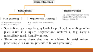
1. • Spatial filtering change the grey level of a pixel (x,y) depending on the
pixel values in a square neighborhood centered at (x,y) using a
matrix(filter, mask, kernel/window).
• There are many things that can be achieved by neighborhood
processing which are not possible with point processing.
Image Enhancement
Spatial domain Frequency domain
Point processing Neighbourhood processing
E.g. Negative Image, contrast
stretching, thresholding etc.
E.g. Averaging filter, median filtering
etc.
E.g. Image sharpening using Gaussian
high pass filters, unsharp masking,
highboost filtering etc.

2. Averaging filter Weighted averaging filter
Minimum filter Maximum filter Median filter
Spatial filters
Smoothing spatial filters (LPF)
Sharpening spatial filters (HPF)
Linear filters Non-linear(Order statistics) spatial filter Laplacian linear filter

3. • Sharpening filters are used to highlight fine details (e.g. edges) in an image, or
enhance details that are blurred through errors or imperfect capturing devices.
• Sharpening is opposite of smoothing(averaging). Hence in mathematics, it is given
by partial derivatives(HPF) as averaging is integration(LPF).
• While linear smoothing is based on the weighted summation or integral
operation on the neighborhood, the sharpening is based on the derivative
(gradient) or finite difference.
• In smoothing we try to smooth noise and ignore edges and in sharpening we try
to enhance edges and ignore noise.
❖ Sharpening Spatial Filters:

4. • The first order partial derivative of the digital image f(x,y) are:
❖ Partial derivatives of digital image:
• The first derivative must be:
(1) Zero along flat segments (i.e. constant grey levels)
(2) Non-zero at the outset of grey level step or ramp (edges or noise)
(3) Non-zero along segments of continuing changes (i.e. ramps)
• The second order partial derivatives of the digital image f(x,y) are:
• The second derivative must be:
(1) Zero along flat segments (i.e. constant grey levels)
(2) Non-zero at the outset of grey level step or ramp (edges or noise)
(3) Zero along ramps.

5. • The first derivative detects thick
edges while second derivative detects
thin edges.
• Second derivative has much stronger
response at grey level step than first
derivative.
• Thus we can expect a second order
derivative to enhance fine detail (thin
lines, edges, including noise) much
more than a first order derivative.
f ' = f(x+1) - f(x)
f '' = f(x+1) + f(x-1) - 2f(x)

6. • The Laplacian operator of an image f(x,y) is:
❖ The Laplacian filter:
• This equation can be implemented using the 3 x 3 mask:
• As the Laplacian filter is a linear spatial filter, we can apply it using the same
mechanism of convolution. This will produce a Laplacian image that has grayish
edge lines and other discontinuities, all superimposed on a dark, featureless
background.
• Background features can be “recovered” while still preserving the sharpening
effects of the Laplacian simply by adding the original and Laplacian images.

7. Filter mask
20 20 20 20 20
20 5 20 20 20
20 20 20 20 20
20 20 20 5 20
20 20 20 20 20
0 -15 0 0 0
0 60 0 0 0
0 -15 0 -15 0
0 0 0 60 0
0 0 0 -15 0
Input image Output image