Modified clahe an adaptive algorithm for contrast enhancement of aerial medical and underwater images

International INTERNATIONAL Journal of Computer JOURNAL Engineering OF and COMPUTER Technology (IJCET), ENGINEERING ISSN 0976-6367(Print),
&
ISSN 0976 - 6375(Online), Volume 5, Issue 11, November (2014), pp. 32-47 © IAEME
TECHNOLOGY (IJCET)
ISSN 0976 – 6367(Print)
ISSN 0976 – 6375(Online)
Volume 5, Issue 11, November (2014), pp. 32-47
© IAEME: www.iaeme.com/IJCET.asp
Journal Impact Factor (2014): 8.5328 (Calculated by GISI)
www.jifactor.com
IJCET

© I A E M E

MODIFIED CLAHE: AN ADAPTIVE ALGORITHM FOR
CONTRAST ENHANCEMENT OF AERIAL, MEDICAL
AND UNDERWATER IMAGES
Jharna Majumdar1, Santhosh Kumar K L2
1Dean RD, Prof Head CSE (PG), Nitte Meenakshi Institute of Technology, Bangalore, India,
2Asst Prof, Dept. of CSE (PG), Nitte Meenakshi Institute of Technology, Bangalore, India,
32
ABSTRACT
Image enhancement has been an area of active research for decades. Most of the studies are
aimed at improving the quality of image for better visualization. Contrast Limited Adaptive
Histogram Equalization (CLAHE) is a technique to enhance the visibility of local details of an image
by increasing the contrast of local regions. The algorithm is extensively used by various researches
for applications in medical imagery. The drawback of CLAHE algorithm is the fact that it is not
automatic and needs two input parameters viz., N size of the sub window and CL the clip limit for
the method to work. Unfortunately none of the researchers have done the automatic selection of N
and CL to make the algorithm suitable for any autonomous system. This paper proposes a novel
extension of the conventional CLAHE algorithm, where N and CL are calculated automatically from
the given image data itself thereby making the algorithm fully adaptive. Our proposed algorithm is
used to study the enhancement of aerial, medical and underwater images. To demonstrate the
effectiveness of our algorithm, a set of quality metric parameters are used. In the conventional
CLAHE algorithm, we vary the value of N and CL and use the quality metric parameters to obtain
the best output for a given combination of N and CL. It is observed that for a given set input images,
the best results obtained using conventional CLAHE algorithm exactly matches with the results
obtained using our algorithm, where N and CL are calculated automatically.
Keywords: Image enhancement, Histogram Equalization, Contrast Limited Adaptive Histogram
Equalization, Adaptively Clipped Contrast Limited Adaptive Histogram Equalization (ACCLAHE),
Fully Automatic Contrast Limited Adaptive Histogram Equalization (Auto-CLAHE), Quality Metric
parameters.

International Journal of Computer Engineering and Technology (IJCET), ISSN 0976-6367(Print),
33
I. INTRODUCTION
Image enhancement, a well-known image preprocessing technique is used to improve the
appearance of an image and make it suitable for human visual perception or subsequent machine
learning. Commonly used image enhancement techniques fall into three different categories: (1)
Global enhancement (2) Local enhancement and (3) Adaptive Enhancement.
The paper consists of the following:
a) Adaptive enhancement techniques such as Adaptive Histogram Equalization [1], Contrast Limited
Adaptive Histogram Equalization (CLAHE) [1, 2] are widely used by researchers [3-6] [13-16]
b) We have proposed some modifications in the existing CLAHE algorithm and made it completely
adaptive and suitable for autonomous application. Proposed two new algorithms Adaptively Clipped
Contrast Limited Adaptive Histogram Equalization (ACCLAHE) and Fully Automatic Contrast
Limited Adaptive Histogram Equalization (AUTO CLAHE) are adaptive and completely suitable for
autonomous application.
c) We have studied the results of enhancement using a number of Quality Metric parameters.
d) We have used aerial, medical and underwater images for our experimental study and analysis of
results.
II. GLOBAL, LOCAL AND ADAPTIVE ENHANCEMENT METHODS
Histogram processing methods are global processing, in the sense that pixels are modified by
a transformation function based on the gray-level content of the entire image. An example of this is
Histogram Equalization. A local enhancement algorithm acts on local regions within an image. The
mapping applied on each pixel in the input image is decided upon by some property of the
neighborhood of that pixel. The methods vary from each other depending on the property chosen and
in the form in which it appears in the mapping. In such methods the size of the neighborhood or the
window size can be varied. Many enhancement algorithms require the user to choose some input
parameter(s) for enhancement. The enhancement is said to be adaptive, if the algorithm chooses the
optimum parameter(s) depending on the properties of the input image.
A. HISTOGRAM EQUALIZATION (HE)
Histogram equalization [5] is one of the well-known method for enhancing the contrast of
given images, making the result image have a uniform distribution of the gray levels. It flattens and
stretches the dynamic range of the image’s histogram and results in overall contrast improvement.
HE has been widely applied when the image needs enhancement however, it may significantly
change the brightness of an input image and cause problem in some applications where brightness
preservation is necessary. Since the HE is based on the whole information of input image to
implement, the local details with smaller probability would not be enhanced.
B. ADAPTIVE HISTOGRAM EQUALIZATION (AHE)
AHE is an extension to traditional Histogram Equalization technique. Unlike HE, it operates
on small data regions (tiles), rather than the entire image. The contrast of each region is enhanced, so
that the histogram of the output region approximately matches the specified histogram. The
neighboring regions are then combined using bilinear interpolation in order to eliminate artificially
induced boundaries [5]. In adaptive histogram equalization, the main idea is to take into account
histogram distribution over local window and combine it with global histogram distribution. The size
of the neighbourhood region is a parameter of the method. It constitutes a characteristic length scale:

contrast at smaller scales is enhanced, while contrast at larger scales is reduced. When the image
region containing a pixel's neighbourhood is fairly homogeneous, its histogram will be strongly
peaked, and the transformation function will map a narrow range of pixel values to the whole range
of the result image. This causes AHE to over amplify small amounts of noise in largely
homogeneous regions of the image [1].
C. CONTRAST LIMITED ADAPTIVE HISTOGRAM EQUALIZATION (CLAHE)
CLAHE is an adaptive contrast enhancement method. It is based on AHE, where the
histogram is calculated for the contextual region of a pixel. The pixel's intensity is thus transformed
to a value within the display range proportional to the pixel intensity's rank in the local intensity
histogram [1]. CLAHE, proposed by Zuierveld et al [2] has two key parameters: block size (N) and
clip limit (CL). These parameters are mainly used to control image quality, but have been
heuristically determined by users. CLAHE was originally developed for medical imaging [1].
CLAHE also had been claimed to improve the contrast better in the underwater [4, 12, and 13] and
aerial image enhancement [6].
34
III. THE PROPOSED METHODS
In this section, we describe two new proposed algorithms Adaptively Clipped Contrast
Limited Adaptive Histogram Equalization (ACCLAHE) and Fully Automatic Contrast Limited
Adaptive Histogram Equalization (Auto-CLAHE) in detail.
A. ADAPTIVELY CLIPPED CONTRAST LIMITED ADAPTIVE HISTOGRAM
EQUALIZATION (ACCLAHE)
We have found that the choice of clip limit is very crucial for optimal enhancement using
CLAHE. The correct choice of the clip level depends very much on the size of the bins in the local
histogram. In our proposed algorithm ACCLAHE, the estimation of the clip limit (CL) value is done
automatically from the given input image. We take the maximum bin height in the local histogram of
the sub-image and redistribute the clipped pixels equally to each gray-level. The ACCLAHE method,
however, is not fully automated as it still needs the value of N as a user input.
Algorithm 1: Adaptively Clipped Contrast Limited Adaptive Histogram Equalization(ACCLAHE)
Input: Image file, N;
Output: ACCLAHE Enhanced Image;
STEPS:
1. Divide the input image into an NxN matrix of sub-images
2. For each sub-image do the following:
2.1 Compute the histogram of the sub-image
2.2 Compute the high peak value of the sub-image
2.3 Calculate the nominal clipping level, P from 0 to high peak using the binary search.
2.4 For each gray level bin in the histogram do the following:
(a) If the histogram bin is greater than the nominal clip level P, clip the histogram to the
nominal clip level P
(b) Collect the number of pixels in the sub-image that caused the histogram bin to exceed
the nominal clip level(P).
2.5 Distribute the clipped pixels uniformly in all histogram bins to obtain the renormalized
clipped histogram.

2.6 Equalize the above histogram to obtain the clipped HE mapping for the sub-image
3. For each pixel in the input image, do the following
3.1 If the pixel belongs to an internal region (IR), then
(a) Compute four weights, one for each of the four nearest sub-images, based on the
proximity of the pixel to the centers of the four nearest sub-images (nearer the center of
the sub-image, larger the weight ).
(b) Calculate the output mapping for the pixel as the weighted sum of the clipped HE
mappings for the four nearest sub-images using the weights computed above.
3.2 If the pixel belongs to an border region (BR), then
(a) Compute two weights, one for each of the two nearest sub-images, based on the
proximity of the pixel to the centers of the two nearest sub-images
mappings for the two nearest sub-images using the weights computed above.
3.3 If the pixel belongs to a corner region (CR), the output mapping for the pixel is the
clipped HE mapping for the sub-image that contains the pixel.
4. Apply the output mapping obtained to each of the pixels in the input image to obtain the image
enhanced by ACCLAHE.
B. FULLY AUTOMATIC CONTRAST LIMITED ADAPTIVE HISTOGRAM
35
EQUALIZATION (Auto-CLAHE)
We propose a method to fully automate the method of enhancement by estimating the value
of N from the global and local entropy in the input image. To each value of N, from N=2 (in which
case, the input image is divided into 2 x 2 = 4 sub-images) to N=12 (in which case, the input image
is divided into 12 x12 = 144 sub-images), we associate the maximum entropy over all the sub-images
of the same size. Now we choose that value of N that is associated with maximum entropy.
For the estimation of CL we follow the ACCLAHE method. We call this method of Auto CLAHE,
since both the input parameters N and CL are automatically estimated.
Algorithm 2: AUTO-CLAHE
Input: Image file;
Output: AUTO-CLAHE Enhanced Image
STEPS:
1. For n=0 to n=12 store entropy[n] = 0.
2. For n = 2 to n = 12, divide the image into n x n matrix of sub-images and store the maximum
entropy of the 2n sub-images as entropy[n].
3. Set N to that value of n for which entropy[n] is maximum.
4. Divide the input image into an NxN matrix of sub-images
5. For each sub-image do the following:
5.1 Compute the histogram of the sub-image.
5.2 Compute the high peak value of the sub-image.
5.3 Calculate the nominal clipping level, P from 0 to high peak using the binary search
elaborated.
5.4 For each gray level bin in the histogram do the following
(a) If the histogram bin is greater than the nominal clip level P, clip the histogram to the
nominal clip level P
(b) Collect the number of pixels in the sub-image that caused the histogram bin to exceed
the nominal clip level.
5.5 Distribute the clipped pixels uniformly in all histogram bins to obtain the renormalized
clipped histogram.

5.6 Equalize the above histogram to obtain the clipped HE mapping for the sub-image
6. For each pixel in the input image, do the following
6.1 If the pixel belongs to an internal region (IR), then
(a) Compute four weights, one for each of the four nearest sub-images, based on the
proximity of the pixel to the centers of the four nearest sub-images (nearer the center of
the sub-image, larger the weight)
mappings for the four nearest sub-images using the weights computed above.
6.2 If the pixel belongs to an border region (BR), then
(a) Compute two weights, one for each of the two nearest sub-images, based on the
proximity of the pixel to the centers of the two nearest sub-images
mappings for the two nearest sub-images using the weights computed above.
6.3 If the pixel belongs to a corner region (CR), the output mapping for the pixel is the HE
mapping for the sub-image that contains the pixel.
7. Apply the output mapping obtained to each of the pixels in the input image to obtain the image
enhanced by Auto-CLAHE.
IV. EXPERIMENTAL STUDY, RESULTS DISCUSSION
All the algorithms presented in this paper are implemented in the Windows 7 – Microsoft
Visual Studio platform using VC++ language for programming. The aerial, medical and underwater
images are selected for study. A set of quality metric parameters such as Entropy [7], Global
Contrast (GC) [8], Spatial Frequency (SF) [9], Fitness Measure (FM) [10] and Absolute Mean
Brightness Error (AMBE) [11] used to measure the quality of the enhanced image with respect to the
original image. The formulas of quality parameters are given in Appendix (section VIII).
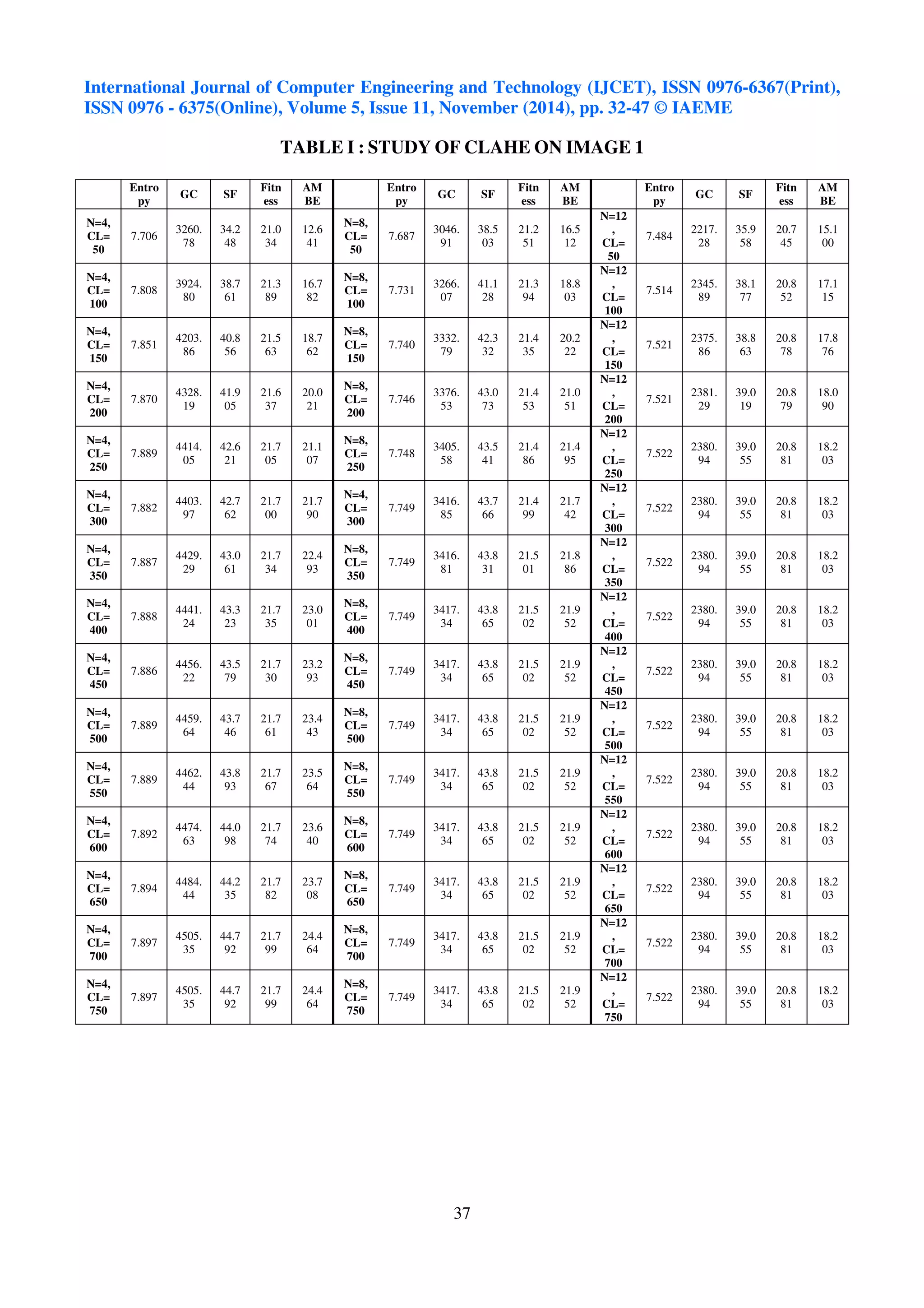
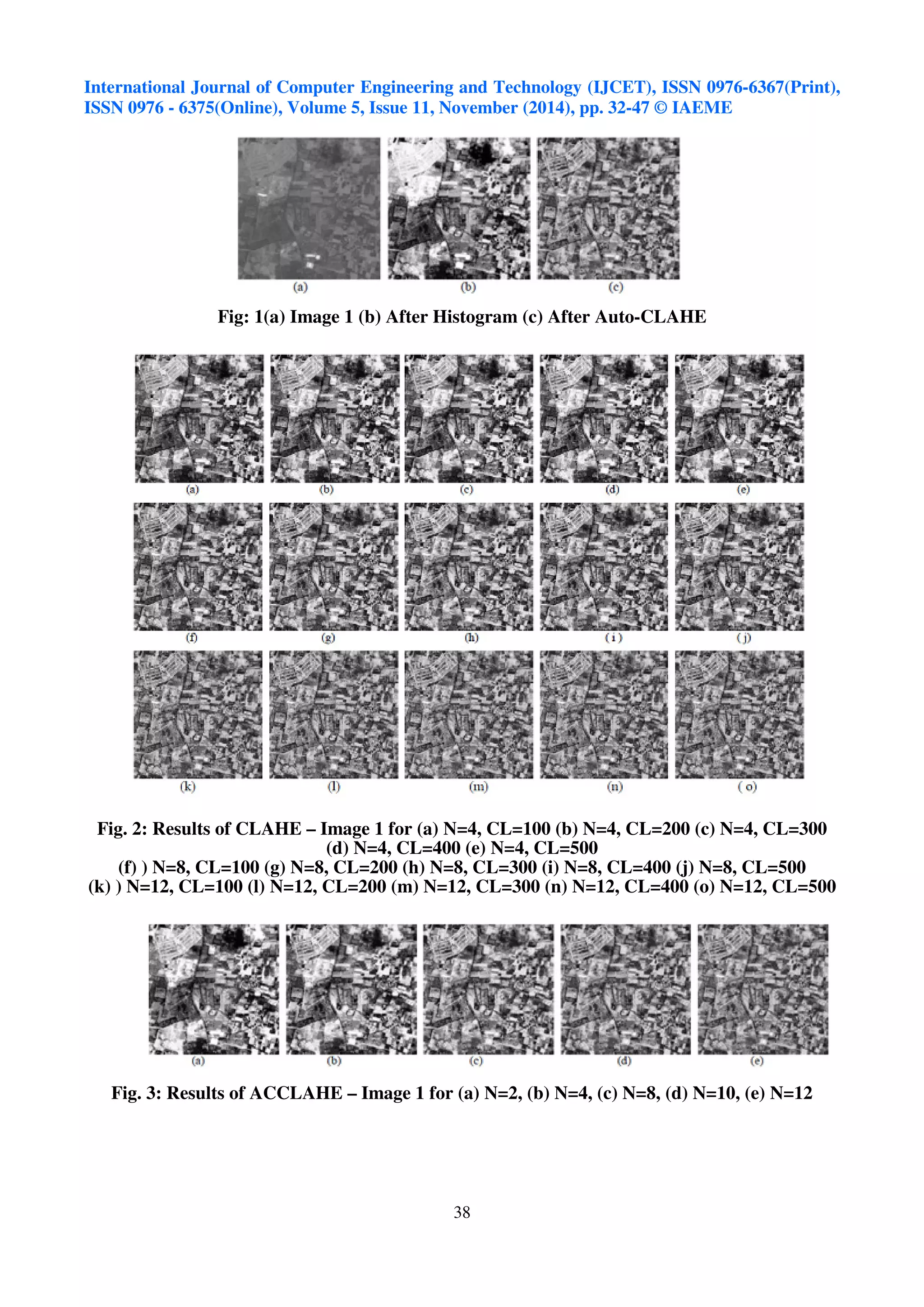
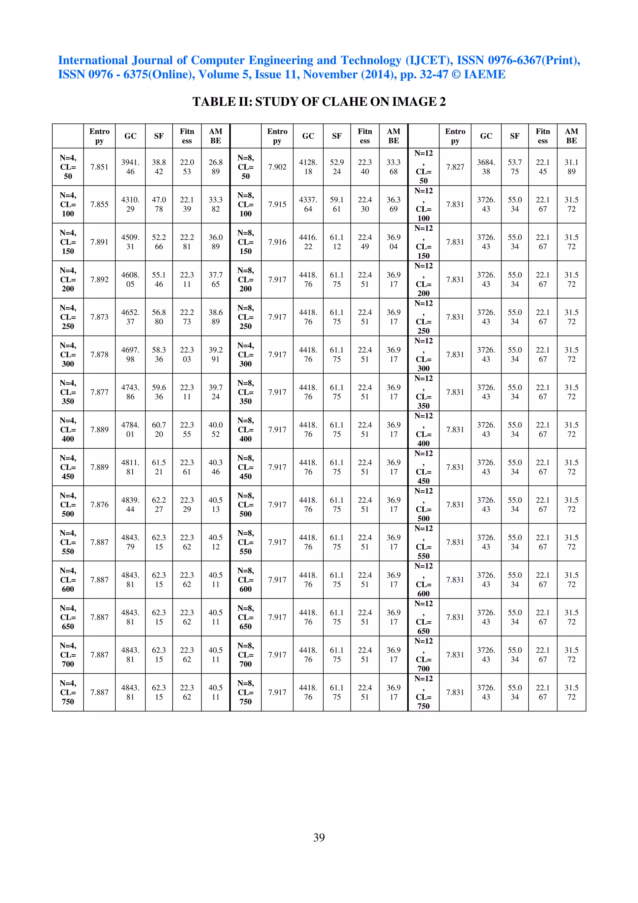
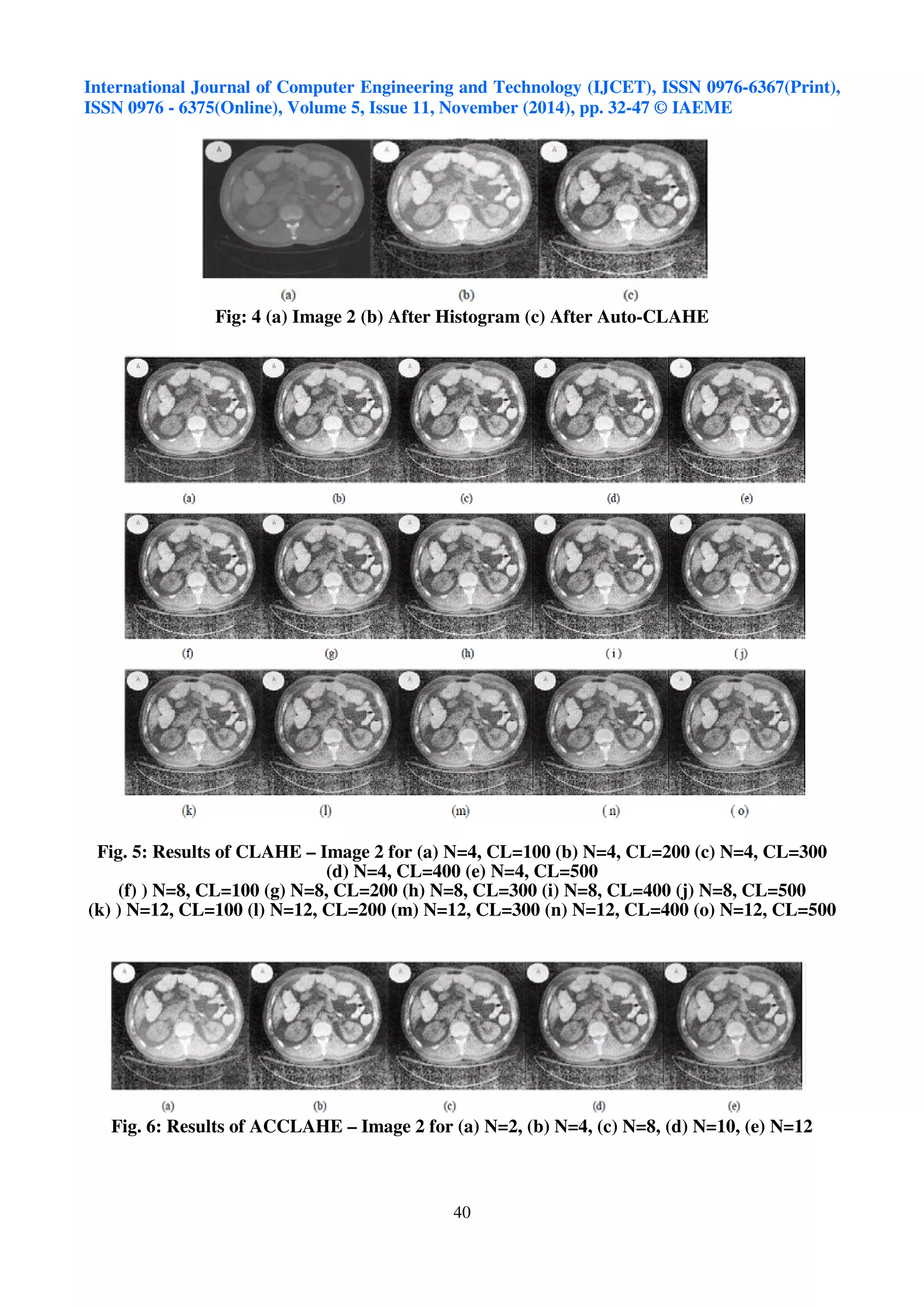
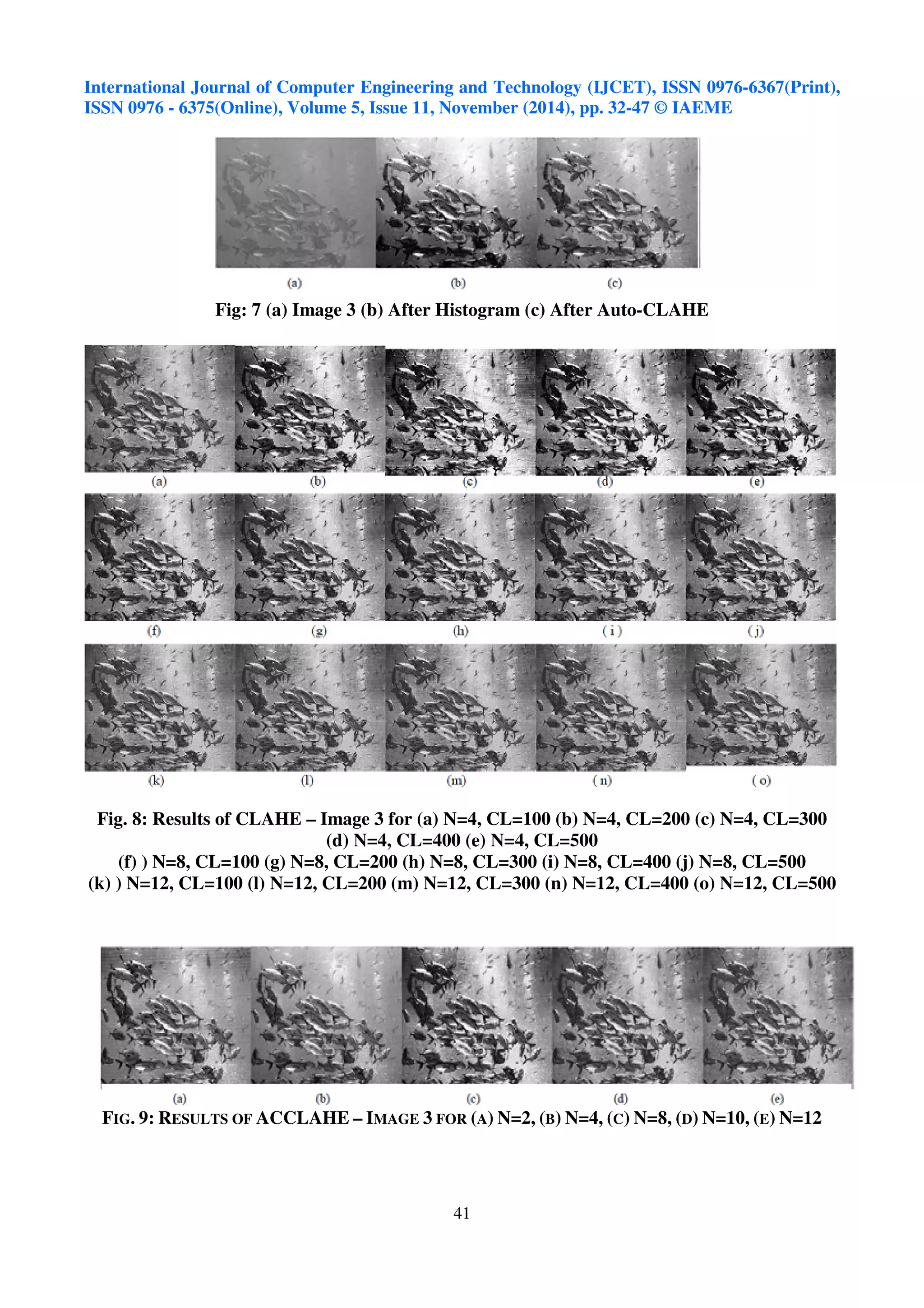
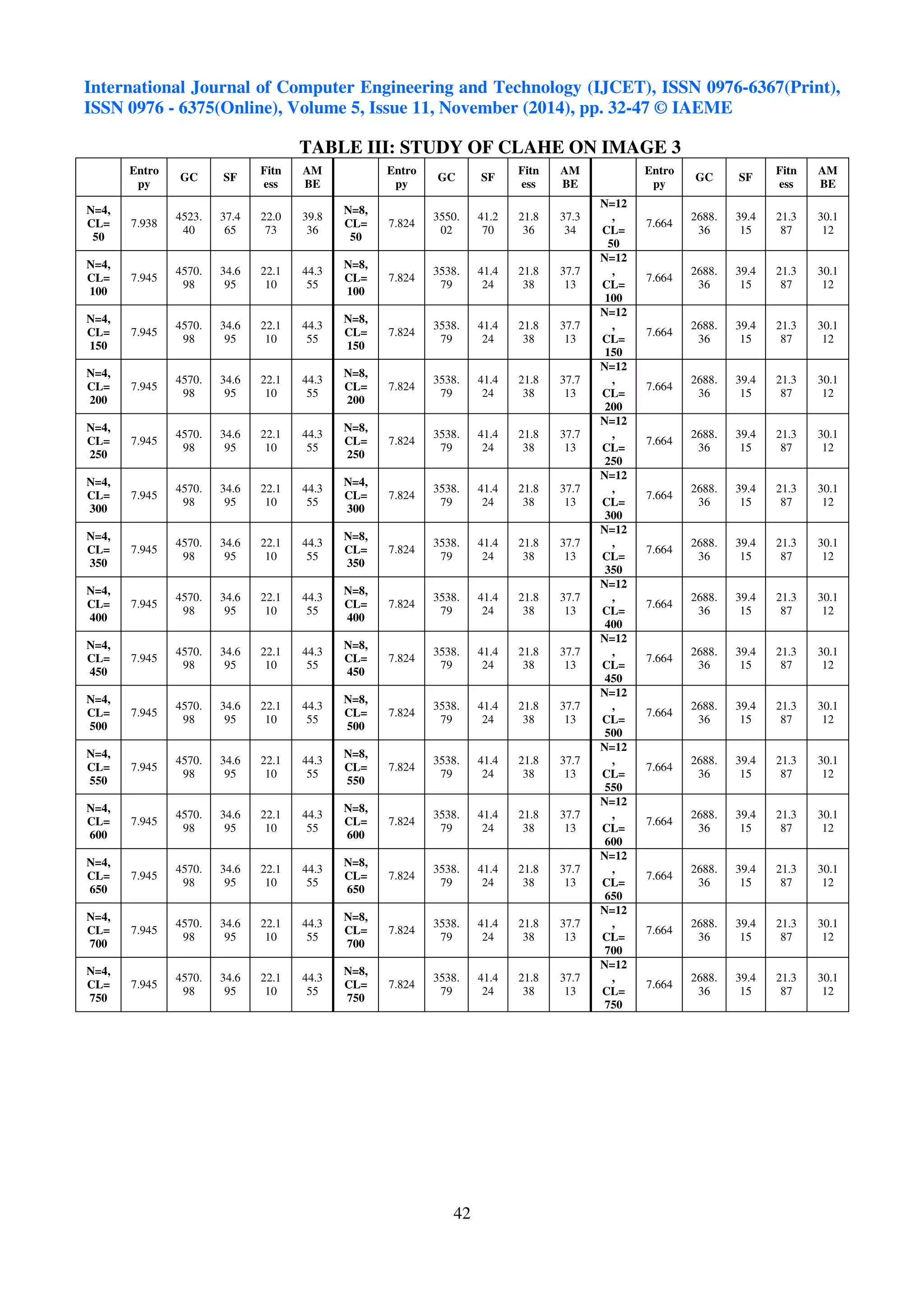
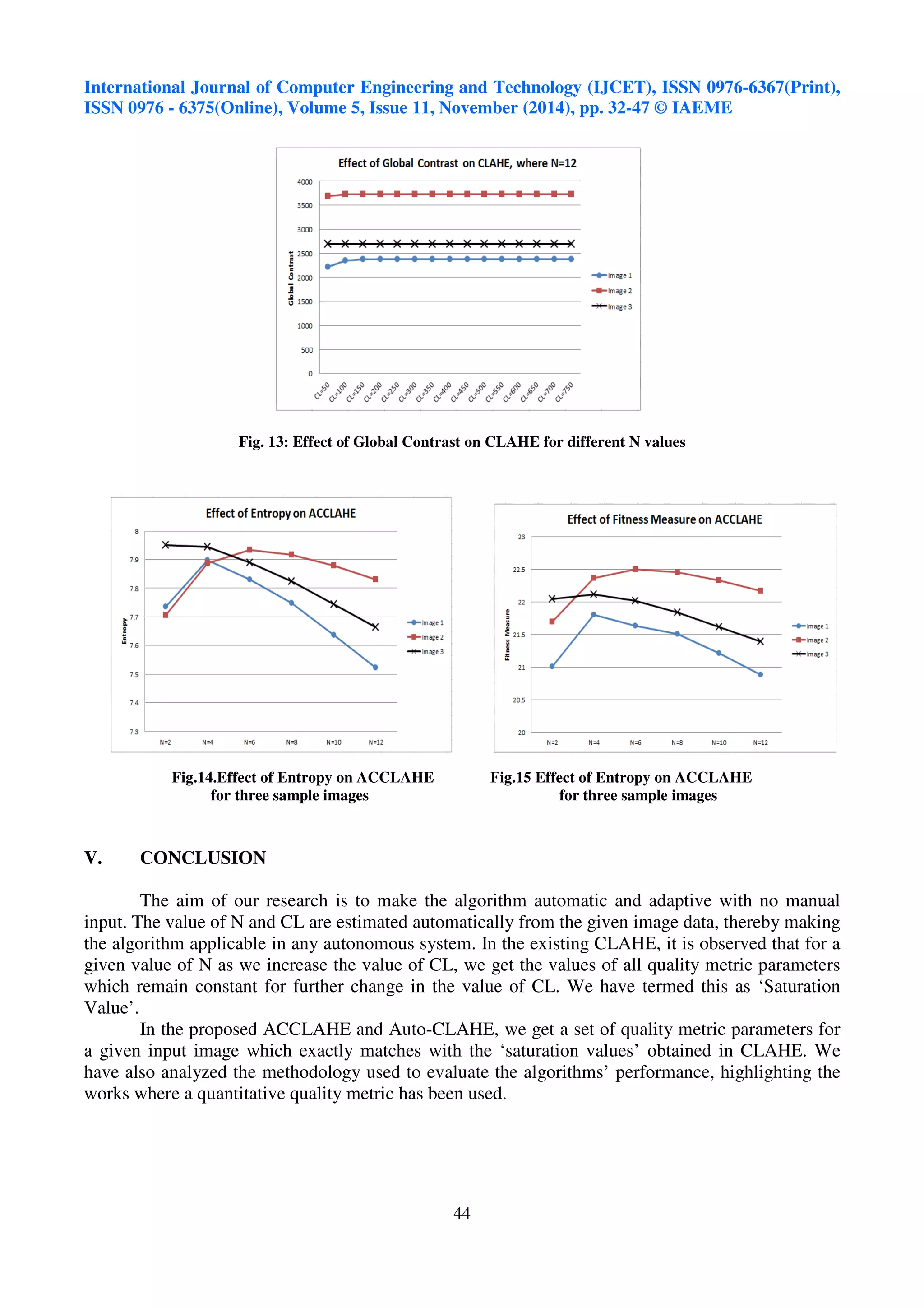
In Contrast Limited Adaptive Histogram Equalization (CLAHE), we have two input
parameters N and CL. The value of N is initially kept constant at N=4 and the value of CL is varied
from 50 to 750 in steps of 50. The experiment is repeated for the value of N=4, 8 and 12. Analysis of
the results show that for a given value of N as we increase the value of CL, after a certain value of
CL, all quality metric parameters reaches to saturation and remains constant throughout the scale as
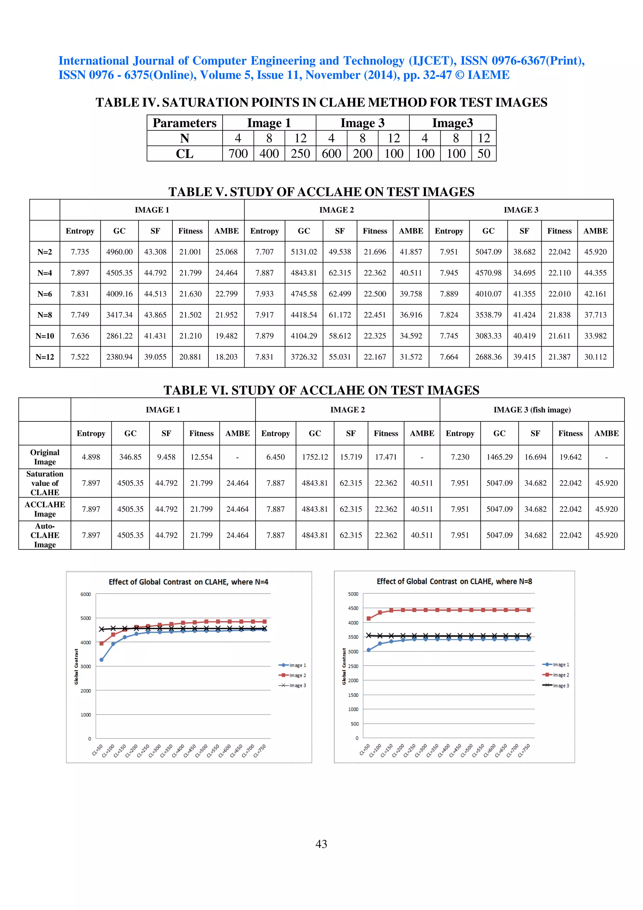
shown in Table I,II,III and sample graphs shown for Global Contrast in Fig 13. The saturation value
of clip limit for a given image is not the same for all the values of N. It is seen that as we increase the
value of N, the optimum value of clip limit that gives the best enhancement result decreases as
evident from the Table IV. The reason may be attributed as follows: As we increase the value of N,
the size of the sub-image decreases. This implies a decrease in the number of pixels in the sub-image
and thus a lowering of the maximum bin height in the local histogram.
In the proposed “Adaptively Clipped Contrast Limited Adaptive Histogram Equalization”
(ACCLAHE) method, N is given as manual input and CL is estimated automatically. The value of N
is varied from 2 to 12 in steps of 2. It is seen from the Table V that the value of all quality
parameters increases initially and subsequently decreases after a certain value of N as shown for
Entropy and Fitness measure in Figs 14-15. The point where the quality parameters reaches
maximum value matches exactly with the saturation value obtained in CLAHE. This fact is observed
for all images used in our experiment.
In the proposed “Fully Automatic Contrast Limited Adaptive Histogram Equalization”
(Auto-CLAHE) method, the values of N and CL are estimated automatically. The effects of quality
metric parameters on the output image after enhancement are studied. It is seen that the saturation
value of CLAHE and ACCLAHE exactly matches with the results obtained using Auto-CLAHE as
shown in Table VI.
36

TABLE I : STUDY OF CLAHE ON IMAGE 1
37
Entro
py
GC SF
Fitn
ess
AM
BE
Entro
py
GC SF
Fitn
ess
AM
BE
Entro
py
GC SF
Fitn
ess
AM
BE
N=4,
CL=
50
7.706
3260.
78
34.2
48
21.0
34
12.6
41
N=8,
CL=
50
7.687
3046.
91
38.5
03
21.2
51
16.5
12
N=12
,
CL=
50
7.484
2217.
28
35.9
58
20.7
45
15.1
00
N=4,
CL=
100
7.808
3924.
80
38.7
61
21.3
89
16.7
82
N=8,
CL=
100
7.731
3266.
07
41.1
28
21.3
94
18.8
03
N=12
,
CL=
100
7.514
2345.
89
38.1
77
20.8
52
17.1
15
N=4,
CL=
150
7.851
4203.
86
40.8
56
21.5
63
18.7
62
N=8,
CL=
150
7.740
3332.
79
42.3
32
21.4
35
20.2
22
N=12
,
CL=
150
7.521
2375.
86
38.8
63
20.8
78
17.8
76
N=4,
CL=
200
7.870
4328.
19
41.9
05
21.6
37
20.0
21
N=8,
CL=
200
7.746
3376.
53
43.0
73
21.4
53
21.0
51
N=12
,
CL=
200
7.521
2381.
29
39.0
19
20.8
79
18.0
90
N=4,
CL=
250
7.889
4414.
05
42.6
21
21.7
05
21.1
07
N=8,
CL=
250
7.748
3405.
58
43.5
41
21.4
86
21.4
95
N=12
,
CL=
250
7.522
2380.
94
39.0
55
20.8
81
18.2
03
N=4,
CL=
300
7.882
4403.
97
42.7
62
21.7
00
21.7
90
N=4,
CL=
300
7.749
3416.
85
43.7
66
21.4
99
21.7
42
N=12
,
CL=
300
7.522
2380.
94
39.0
55
20.8
81
18.2
03
N=4,
CL=
350
7.887
4429.
29
43.0
61
21.7
34
22.4
93
N=8,
CL=
350
7.749
3416.
81
43.8
31
21.5
01
21.8
86
N=12
,
CL=
350
7.522
2380.
94
39.0
55
20.8
81
18.2
03
N=4,
CL=
400
7.888
4441.
24
43.3
23
21.7
35
23.0
01
N=8,
CL=
400
7.749
3417.
34
43.8
65
21.5
02
21.9
52
N=12
,
CL=
400
7.522
2380.
94
39.0
55
20.8
81
18.2
03
N=4,
CL=
450
7.886
4456.
22
43.5
79
21.7
30
23.2
93
N=8,
CL=
450
7.749
3417.
34
43.8
65
21.5
02
21.9
52
N=12
,
CL=
450
7.522
2380.
94
39.0
55
20.8
81
18.2
03
N=4,
CL=
500
7.889
4459.
64
43.7
46
21.7
61
23.4
43
N=8,
CL=
500
7.749
3417.
34
43.8
65
21.5
02
21.9
52
N=12
,
CL=
500
7.522
2380.
94
39.0
55
20.8
81
18.2
03
N=4,
CL=
550
7.889
4462.
44
43.8
93
21.7
67
23.5
64
N=8,
CL=
550
7.749
3417.
34
43.8
65
21.5
02
21.9
52
N=12
,
CL=
550
7.522
2380.
94
39.0
55
20.8
81
18.2
03
N=4,
CL=
600
7.892
4474.
63
44.0
98
21.7
74
23.6
40
N=8,
CL=
600
7.749
3417.
34
43.8
65
21.5
02
21.9
52
N=12
,
CL=
600
7.522
2380.
94
39.0
55
20.8
81
18.2
03
N=4,
CL=
650
7.894
4484.
44
44.2
35
21.7
82
23.7
08
N=8,
CL=
650
7.749
3417.
34
43.8
65
21.5
02
21.9
52
N=12
,
CL=
650
7.522
2380.
94
39.0
55
20.8
81
18.2
03
N=4,
CL=
700
7.897
4505.
35
44.7
92
21.7
99
24.4
64
N=8,
CL=
700
7.749
3417.
34
43.8
65
21.5
02
21.9
52
N=12
,
CL=
700
7.522
2380.
94
39.0
55
20.8
81
18.2
03
N=4,
CL=
750
7.897
4505.
35
44.7
92
21.7
99
24.4
64
N=8,
CL=
750
7.749
3417.
34
43.8
65
21.5
02
21.9
52
N=12
,
CL=
750
7.522
2380.
94
39.0
55
20.8
81
18.2
03

Fig: 1(a) Image 1 (b) After Histogram (c) After Auto-CLAHE
Fig. 2: Results of CLAHE – Image 1 for (a) N=4, CL=100 (b) N=4, CL=200 (c) N=4, CL=300
(d) N=4, CL=400 (e) N=4, CL=500
(f) ) N=8, CL=100 (g) N=8, CL=200 (h) N=8, CL=300 (i) N=8, CL=400 (j) N=8, CL=500
(k) ) N=12, CL=100 (l) N=12, CL=200 (m) N=12, CL=300 (n) N=12, CL=400 (o) N=12, CL=500
Fig. 3: Results of ACCLAHE – Image 1 for (a) N=2, (b) N=4, (c) N=8, (d) N=10, (e) N=12
38

TABLE II: STUDY OF CLAHE ON IMAGE 2
39
Entro
py
GC SF
Fitn
ess
AM
BE
Entro
py
GC SF
Fitn
ess
AM
BE
Entro
py
GC SF
Fitn
ess
AM
BE
N=4,
CL=
50
7.851
3941.
46
38.8
42
22.0
53
26.8
89
N=8,
CL=
50
7.902
4128.
18
52.9
24
22.3
40
33.3
68
N=12
,
CL=
50
7.827
3684.
38
53.7
75
22.1
45
31.1
89
N=4,
CL=
100
7.855
4310.
29
47.0
78
22.1
39
33.3
82
N=8,
CL=
100
7.915
4337.
64
59.1
61
22.4
30
36.3
69
N=12
,
CL=
100
7.831
3726.
43
55.0
34
22.1
67
31.5
72
N=4,
CL=
150
7.891
4509.
31
52.2
66
22.2
81
36.0
89
N=8,
CL=
150
7.916
4416.
22
61.1
12
22.4
49
36.9
04
N=12
,
CL=
150
7.831
3726.
43
55.0
34
22.1
67
31.5
72
N=4,
CL=
200
7.892
4608.
05
55.1
46
22.3
11
37.7
65
N=8,
CL=
200
7.917
4418.
76
61.1
75
22.4
51
36.9
17
N=12
,
CL=
200
7.831
3726.
43
55.0
34
22.1
67
31.5
72
N=4,
CL=
250
7.873
4652.
37
56.8
80
22.2
73
38.6
89
N=8,
CL=
250
7.917
4418.
76
61.1
75
22.4
51
36.9
17
N=12
,
CL=
250
7.831
3726.
43
55.0
34
22.1
67
31.5
72
N=4,
CL=
300
7.878
4697.
98
58.3
36
22.3
03
39.2
91
N=4,
CL=
300
7.917
4418.
76
61.1
75
22.4
51
36.9
17
N=12
,
CL=
300
7.831
3726.
43
55.0
34
22.1
67
31.5
72
N=4,
CL=
350
7.877
4743.
86
59.6
36
22.3
11
39.7
24
N=8,
CL=
350
7.917
4418.
76
61.1
75
22.4
51
36.9
17
N=12
,
CL=
350
7.831
3726.
43
55.0
34
22.1
67
31.5
72
N=4,
CL=
400
7.889
4784.
01
60.7
20
22.3
55
40.0
52
N=8,
CL=
400
7.917
4418.
76
61.1
75
22.4
51
36.9
17
N=12
,
CL=
400
7.831
3726.
43
55.0
34
22.1
67
31.5
72
N=4,
CL=
450
7.889
4811.
81
61.5
21
22.3
61
40.3
46
N=8,
CL=
450
7.917
4418.
76
61.1
75
22.4
51
36.9
17
N=12
,
CL=
450
7.831
3726.
43
55.0
34
22.1
67
31.5
72
N=4,
CL=
500
7.876
4839.
44
62.2
27
22.3
29
40.5
13
N=8,
CL=
500
7.917
4418.
76
61.1
75
22.4
51
36.9
17
N=12
,
CL=
500
7.831
3726.
43
55.0
34
22.1
67
31.5
72
N=4,
CL=
550
7.887
4843.
79
62.3
15
22.3
62
40.5
12
N=8,
CL=
550
7.917
4418.
76
61.1
75
22.4
51
36.9
17
N=12
,
CL=
550
7.831
3726.
43
55.0
34
22.1
67
31.5
72
N=4,
CL=
600
7.887
4843.
81
62.3
15
22.3
62
40.5
11
N=8,
CL=
600
7.917
4418.
76
61.1
75
22.4
51
36.9
17
N=12
,
CL=
600
7.831
3726.
43
55.0
34
22.1
67
31.5
72
N=4,
CL=
650
7.887
4843.
81
62.3
15
22.3
62
40.5
11
N=8,
CL=
650
7.917
4418.
76
61.1
75
22.4
51
36.9
17
N=12
,
CL=
650
7.831
3726.
43
55.0
34
22.1
67
31.5
72
N=4,
CL=
700
7.887
4843.
81
62.3
15
22.3
62
40.5
11
N=8,
CL=
700
7.917
4418.
76
61.1
75
22.4
51
36.9
17
N=12
,
CL=
700
7.831
3726.
43
55.0
34
22.1
67
31.5
72
N=4,
CL=
750
7.887
4843.
81
62.3
15
22.3
62
40.5
11
N=8,
CL=
750
7.917
4418.
76
61.1
75
22.4
51
36.9
17
N=12
,
CL=
750
7.831
3726.
43
55.0
34
22.1
67
31.5
72

Fig: 4 (a) Image 2 (b) After Histogram (c) After Auto-CLAHE
40

(d) N=4, CL=400 (e) N=4, CL=500
Fig. 6: Results of ACCLAHE – Image 2 for (a) N=2, (b) N=4, (c) N=8, (d) N=10, (e) N=12

Fig: 7 (a) Image 3 (b) After Histogram (c) After Auto-CLAHE
(d) N=4, CL=400 (e) N=4, CL=500
FIG. 9: RESULTS OF ACCLAHE – IMAGE 3 FOR (A) N=2, (B) N=4, (C) N=8, (D) N=10, (E) N=12
41

TABLE III: STUDY OF CLAHE ON IMAGE 3
42
Entro
py
GC SF
Fitn
ess
AM
BE
Entro
py
GC SF
Fitn
ess
AM
BE
Entro
py
GC SF
Fitn
ess
AM
BE
N=4,
CL=
50
7.938
4523.
40
37.4
65
22.0
73
39.8
36
N=8,
CL=
50
7.824
3550.
02
41.2
70
21.8
36
37.3
34
N=12
,
CL=
50
7.664
2688.
36
39.4
15
21.3
87
30.1
12
N=4,
CL=
100
7.945
4570.
98
34.6
95
22.1
10
44.3
55
N=8,
CL=
100
7.824
3538.
79
41.4
24
21.8
38
37.7
13
N=12
,
CL=
100
7.664
2688.
36
39.4
15
21.3
87
30.1
12
N=4,
CL=
150
7.945
4570.
98
34.6
95
22.1
10
44.3
55
N=8,
CL=
150
7.824
3538.
79
41.4
24
21.8
38
37.7
13
N=12
,
CL=
150
7.664
2688.
36
39.4
15
21.3
87
30.1
12
N=4,
CL=
200
7.945
4570.
98
34.6
95
22.1
10
44.3
55
N=8,
CL=
200
7.824
3538.
79
41.4
24
21.8
38
37.7
13
N=12
,
CL=
200
7.664
2688.
36
39.4
15
21.3
87
30.1
12
N=4,
CL=
250
7.945
4570.
98
34.6
95
22.1
10
44.3
55
N=8,
CL=
250
7.824
3538.
79
41.4
24
21.8
38
37.7
13
N=12
,
CL=
250
7.664
2688.
36
39.4
15
21.3
87
30.1
12
N=4,
CL=
300
7.945
4570.
98
34.6
95
22.1
10
44.3
55
N=4,
CL=
300
7.824
3538.
79
41.4
24
21.8
38
37.7
13
N=12
,
CL=
300
7.664
2688.
36
39.4
15
21.3
87
30.1
12
N=4,
CL=
350
7.945
4570.
98
34.6
95
22.1
10
44.3
55
N=8,
CL=
350
7.824
3538.
79
41.4
24
21.8
38
37.7
13
N=12
,
CL=
350
7.664
2688.
36
39.4
15
21.3
87
30.1
12
N=4,
CL=
400
7.945
4570.
98
34.6
95
22.1
10
44.3
55
N=8,
CL=
400
7.824
3538.
79
41.4
24
21.8
38
37.7
13
N=12
,
CL=
400
7.664
2688.
36
39.4
15
21.3
87
30.1
12
N=4,
CL=
450
7.945
4570.
98
34.6
95
22.1
10
44.3
55
N=8,
CL=
450
7.824
3538.
79
41.4
24
21.8
38
37.7
13
N=12
,
CL=
450
7.664
2688.
36
39.4
15
21.3
87
30.1
12
N=4,
CL=
500
7.945
4570.
98
34.6
95
22.1
10
44.3
55
N=8,
CL=
500
7.824
3538.
79
41.4
24
21.8
38
37.7
13
N=12
,
CL=
500
7.664
2688.
36
39.4
15
21.3
87
30.1
12
N=4,
CL=
550
7.945
4570.
98
34.6
95
22.1
10
44.3
55
N=8,
CL=
550
7.824
3538.
79
41.4
24
21.8
38
37.7
13
N=12
,
CL=
550
7.664
2688.
36
39.4
15
21.3
87
30.1
12
N=4,
CL=
600
7.945
4570.
98
34.6
95
22.1
10
44.3
55
N=8,
CL=
600
7.824
3538.
79
41.4
24
21.8
38
37.7
13
N=12
,
CL=
600
7.664
2688.
36
39.4
15
21.3
87
30.1
12
N=4,
CL=
650
7.945
4570.
98
34.6
95
22.1
10
44.3
55
N=8,
CL=
650
7.824
3538.
79
41.4
24
21.8
38
37.7
13
N=12
,
CL=
650
7.664
2688.
36
39.4
15
21.3
87
30.1
12
N=4,
CL=
700
7.945
4570.
98
34.6
95
22.1
10
44.3
55
N=8,
CL=
700
7.824
3538.
79
41.4
24
21.8
38
37.7
13
N=12
,
CL=
700
7.664
2688.
36
39.4
15
21.3
87
30.1
12
N=4,
CL=
750
7.945
4570.
98
34.6
95
22.1
10
44.3
55
N=8,
CL=
750
7.824
3538.
79
41.4
24
21.8
38
37.7
13
N=12
,
CL=
750
7.664
2688.
36
39.4
15
21.3
87
30.1
12

TABLE IV. SATURATION POINTS IN CLAHE METHOD FOR TEST IMAGES
Parameters Image 1 Image 3 Image3
N 4 8 12 4 8 12 4 8 12
CL 700 400 250 600 200 100 100 100 50
TABLE V. STUDY OF ACCLAHE ON TEST IMAGES
IMAGE 1 IMAGE 2 IMAGE 3
Entropy GC SF Fitness AMBE Entropy GC SF Fitness AMBE Entropy GC SF Fitness AMBE
N=2 7.735 4960.00 43.308 21.001 25.068 7.707 5131.02 49.538 21.696 41.857 7.951 5047.09 38.682 22.042 45.920
N=4 7.897 4505.35 44.792 21.799 24.464 7.887 4843.81 62.315 22.362 40.511 7.945 4570.98 34.695 22.110 44.355
N=6 7.831 4009.16 44.513 21.630 22.799 7.933 4745.58 62.499 22.500 39.758 7.889 4010.07 41.355 22.010 42.161
N=8 7.749 3417.34 43.865 21.502 21.952 7.917 4418.54 61.172 22.451 36.916 7.824 3538.79 41.424 21.838 37.713
N=10 7.636 2861.22 41.431 21.210 19.482 7.879 4104.29 58.612 22.325 34.592 7.745 3083.33 40.419 21.611 33.982
N=12 7.522 2380.94 39.055 20.881 18.203 7.831 3726.32 55.031 22.167 31.572 7.664 2688.36 39.415 21.387 30.112
TABLE VI. STUDY OF ACCLAHE ON TEST IMAGES
IMAGE 1 IMAGE 2 IMAGE 3 (fish image)
Entropy GC SF Fitness AMBE Entropy GC SF Fitness AMBE Entropy GC SF Fitness AMBE
43
Original
Image
4.898 346.85 9.458 12.554 - 6.450 1752.12 15.719 17.471 - 7.230 1465.29 16.694 19.642 -
Saturation
value of
CLAHE
7.897 4505.35 44.792 21.799 24.464 7.887 4843.81 62.315 22.362 40.511 7.951 5047.09 34.682 22.042 45.920
ACCLAHE
Image
7.897 4505.35 44.792 21.799 24.464 7.887 4843.81 62.315 22.362 40.511 7.951 5047.09 34.682 22.042 45.920
Auto-
CLAHE
Image
7.897 4505.35 44.792 21.799 24.464 7.887 4843.81 62.315 22.362 40.511 7.951 5047.09 34.682 22.042 45.920

Fig. 13: Effect of Global Contrast on CLAHE for different N values
Fig.14.Effect of Entropy on ACCLAHE Fig.15 Effect of Entropy on ACCLAHE
for three sample images for three sample images
44
V. CONCLUSION
The aim of our research is to make the algorithm automatic and adaptive with no manual
input. The value of N and CL are estimated automatically from the given image data, thereby making
the algorithm applicable in any autonomous system. In the existing CLAHE, it is observed that for a
given value of N as we increase the value of CL, we get the values of all quality metric parameters
which remain constant for further change in the value of CL. We have termed this as ‘Saturation
Value’.
In the proposed ACCLAHE and Auto-CLAHE, we get a set of quality metric parameters for
a given input image which exactly matches with the ‘saturation values’ obtained in CLAHE. We
have also analyzed the methodology used to evaluate the algorithms’ performance, highlighting the
works where a quantitative quality metric has been used.

45
VI. ACKNOWLEDGMENTS
The authors express their sincere gratitude to Prof. N R Shetty, Director, Nitte Meenakshi
Institute of Technology and Dr. H C Nagaraj, Principal, Nitte Meenakshi Institute of Technology for
providing encouragement, support and the infrastructure to carry out the research.
VII. REFERENCES
[1] Stephen M. Pizer, E. Philip Amburn, John D. Austin, Robert Cromartie, “Adaptive Histogram
Equalization and Its Variations,” Computer Vision, Graphics, And Image Processing 39, 355-
368 (1987)
[2] K. Zuiderveld, “Contrast Limited Adaptive Histogram Equalization”, Academic Press Inc.,
(1994).
[3] Kashif Iqbal, Rosalina Abdul Salam, azam Osman and Abdullah Zawawi Talib, “Underwater
Image Enhancement Using an Integrated Colour Model,” IAENG International Journal of
Computer Science, 34:2, IJCS_34_2_12, 2007
[4] Balvant Singh, Ravi Shankar Mistra, Puran Gour, “Analysis of Contrast Enhancement
Techniques For Underwater Image,” IJCTEE Volume 1, Issue 2, 2009
[5] Rajesh Garg, Bhawna Mittal, sheetal garg, “Histogram Equalization Techniques For Image
Enhancement,” International Journal of Electronics Communication Technology, Volume 2,
Issue 1, March 2011
[6] Ramyashree N, Pathra P, Shruthi T V, Dr. JharnaMajumdar, “Enhacement of Aerial and
Medical Image using Multi resolution pyramid,” Special Issue of IJCCT Vol. 1 Issue 2,3,4;
International Conferecnce - ACCTA-2010
[7] Zhengmao Ye, Objective Assessment of Nonlinear Segmentation Approaches to Gray Level
Underwater Images, ICGST-GVIP Journal, ISSN 1687-398X, Volume (9), Issue (II), April
2009
[8] Jia-Guu Leu, “Image Contrast Enhancement Based on the Intensities of Edge Pixels,”
CVGIP: Graphical Models And Image Processing Vol. 54, No. 6, November, pp. 497-506,
1992.
[9] Sonja Grgi c Mislav Grgic Marta Mrak, “Reliability of Objective Picture Quality Measures,”
Journal of ELECTRICAL ENGINEERING, VOL. 55, NO. 1-2, 2004, 3-10.
[10] Munteanu C and Rosa A, “Gray-Scale Image Enhancement as an Automatic Process Driven
by Evolution,” IEEE Transactions on Systems, Man, and Cybernetics—Part B: Cybernetics,
Vol. 34, No. 2, April 2004.
[11] Iyad Jafar Hao Ying, “A New Method for Image Contrast Enhancement Based on Automatic
Specification of Local Histograms”, IJCSNS International Journal of Computer Science and
Network Security, VOL.7 No.7, July 2007.
[12] Raimondo Schettini and Silvia Corchs, “Review Article - Underwater Image Processing :
State of the Art of restoration and Image Enhancement Methods,” EURASIP Journal on
Advances in Signal Processing, Volume 2010.
[13] Rajesh Kumar Rai, Puran Gour, Balvant Singh, “Underwater Image Segmentation using
CLAHE Enhancement and Thresholding,” International Journal of Emerging Technology and
Advanced Engineering, ISSN 2250-2459, Volume 2, Issue 1, January 2012
[14] Wan Nural Jawahir Hj Wan Yussof, Muhammad Suzuri Hitam, Ezmahamrul Afreen
Awalludin, and Zainuddin Bachok, “Performing Contrast Limited Adaptive Histogram
Equalization Technique on Combined Color Models for Underwater Image Enhancement,”
International Journal of Interactive Digital Media, Vol. 1(1), ISSN 2289-4098, e-ISSN 2289-
4101- 2013

[15] D. P. Sharma “Intensity Transformation using Contrast Limited Adaptive Histogram
Equalization” International Journal of Engineering Research (ISSN: 2319-6890) Volume
No.2, Issue No. 4, pp : 282-285 01 Aug. 2013
[16] Neethu M. Sasi, V. K. Jayasree, “ Contrast Limited Adaptive Histogram Equalization for
Qualitative Enhancement of Myocardial Perfusion Images,” Scientific Research, October
2013
[17] Prathap P and Manjula S, “To Improve Energy-Efficient and Secure Multipath
Communication In Underwater Sensor Network” International journal of Computer
Engineering Technology (IJCET), Volume 5, Issue 2, 2014, pp. 145 - 152, ISSN Print:
0976 – 6367, ISSN Online: 0976 – 6375.
VIII. APPENDIX : QUALITY METRIC PARAMETERS FOR IMAGE ENHANCEMENT
R (4)
C (5)
46
A. ENTROPY:
The entropy [7] also called discrete entropy is a measure of information content in an image
and is given by,
=
Entropy p k p k
=−
255
0 2 ( )log( ( ))
k
(1)
Where p(k) is the probability distribution function. Larger the entropy, larger is the information
contained in the image and hence more details are visible in the image.
B. GLOBAL CONTRAST (GC):
The global contrast [8] value of an image is defined as the second central moment of its
histogram divided by N, the total number of pixels in the image.
( i ) 2 μ* histi
( )
N
GC
L
i
=
−
= 0
(2)
Where, μ is the average intensity of the image, hist(i) is the number of pixels in the image with the
intensity value i and L is the highest intensity value.
C. SPATIAL FREQUENCY(SF):
The Spatial Frequency [9] indicates the overall activity level in an image. SF is defined as
follows:
2 2 SF= R +C (3)
2
M
N
1
− = −
1 2
, , 1( )
j
k
= =
j k j k x x
MN
2
M
− = −
1 2
, 1, ( )
1
= =
k
N
j
j k j k x x
M

Where R is row frequency, C is column frequency and xj,k denotes the pixel intensity values of
image; M and N are numbers of pixels in horizontal and vertical directions.
47
D. FITNESS MEASURE:
The Fitness measure [10] depends on the entropy H(I), no. of edges n(I) and the intensity of
edges E(I).
n I
ln(ln ( ) ) H I
( )
( )
( * )
widthheight
FitnessMseuare= E I +e
(6)
Compared to the original image, the enhanced version should have a higher intensity of the edges.
E. ABSOLUTE MEAN BRIGHTNESS ERROR (AMBE):
AMBE [11] simply measures the deviation of the processed image mean ‘μp’ from the input
image mean ‘μi’
p i AMBE = μ − μ (7)
The AMBE value provides a sense of how the image global appearance has changed, with
preference to lower values.

Modified clahe an adaptive algorithm for contrast enhancement of aerial medical and underwater images

More Related Content

What's hot

Viewers also liked

Similar to Modified clahe an adaptive algorithm for contrast enhancement of aerial medical and underwater images

More from IAEME Publication

Recently uploaded

Modified clahe an adaptive algorithm for contrast enhancement of aerial medical and underwater images