Downloaded 51 times
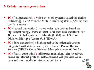
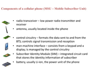
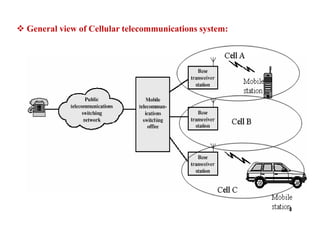
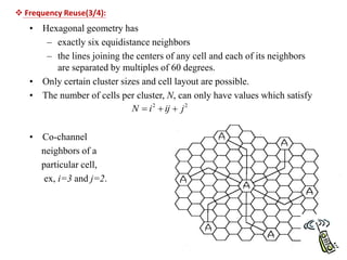
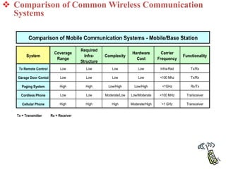
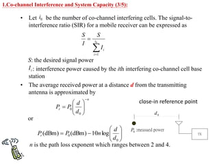
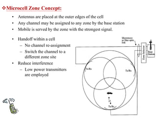
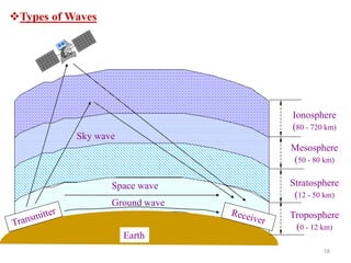
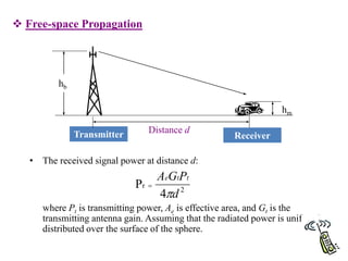
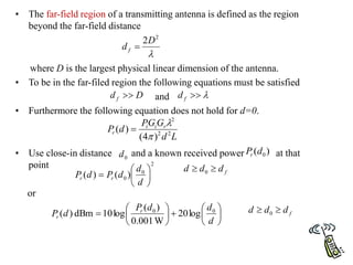
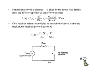
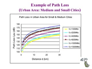
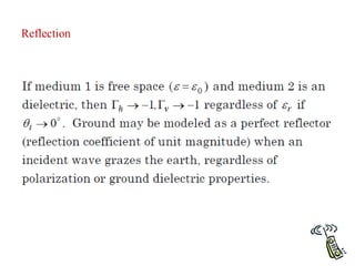
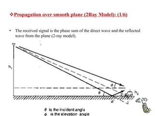
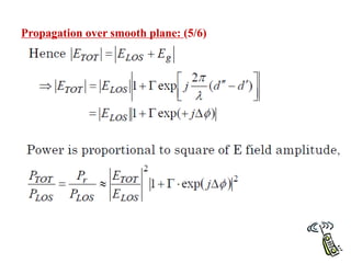
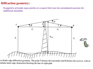
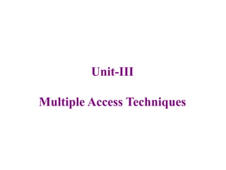
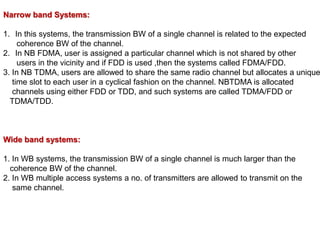
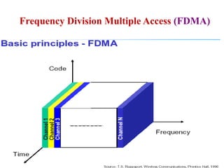
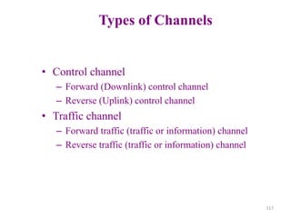
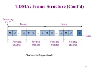
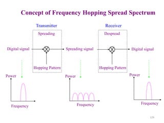
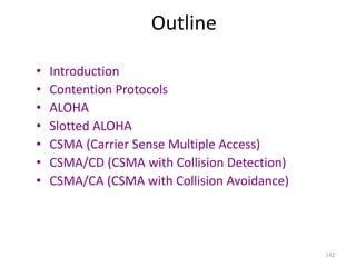
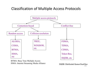
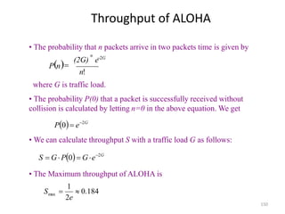
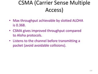
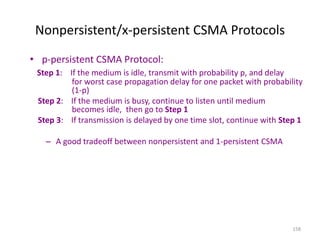
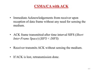
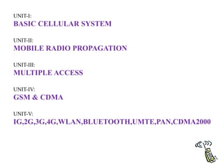
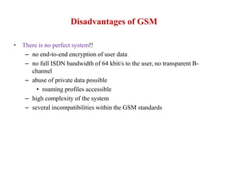
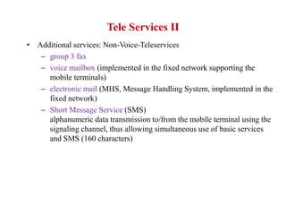
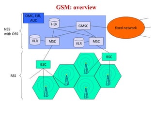
![ Mobile phone subscribers worldwide:
year
Subscribers
[million]
0
200
400
600
800
1000
1200
1400
1600
1996 1997 1998 1999 2000 2001 2002 2003 2004
approx. 1.7 bn
GSM total
TDMA total
CDMA total
PDC total
Analogue total
W-CDMA
Total wireless
Prediction (1998)
2009:
>4 bn!](https://image.slidesharecdn.com/mobilecellularcommunication-230123165246-e8599357/85/Mobile-cellular-Communication-ppt-4-320.jpg)
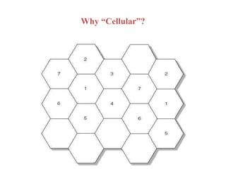
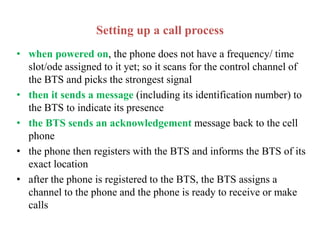
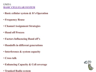
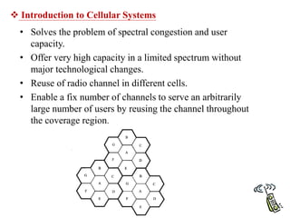
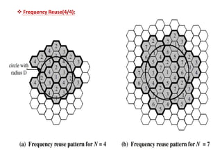
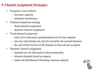
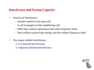
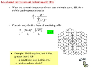
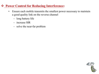
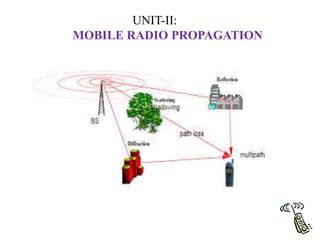
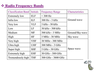
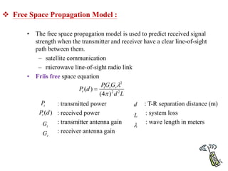
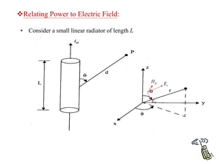
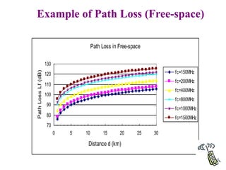
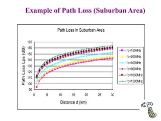
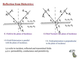
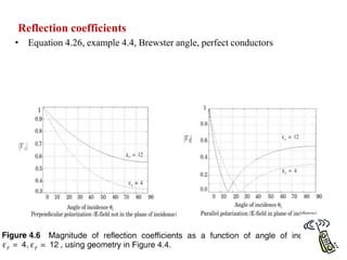
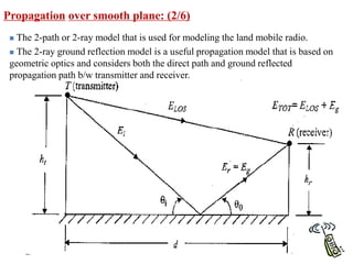
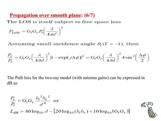
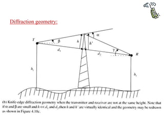
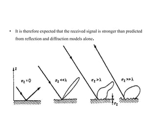
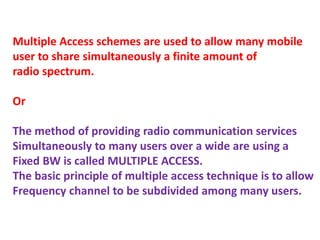
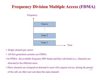
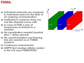
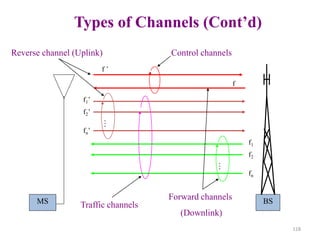
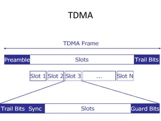
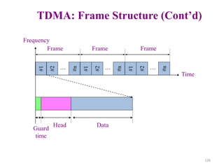
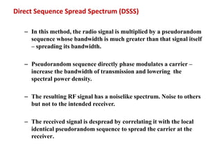
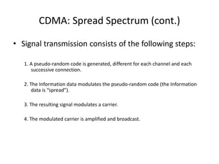
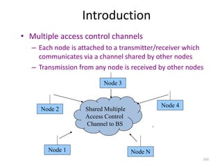
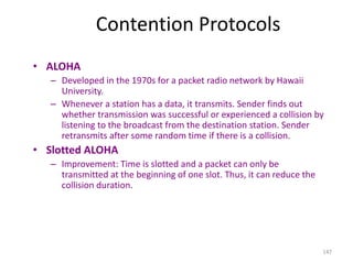
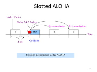
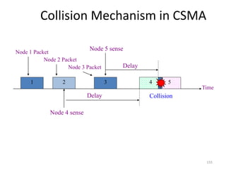
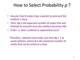
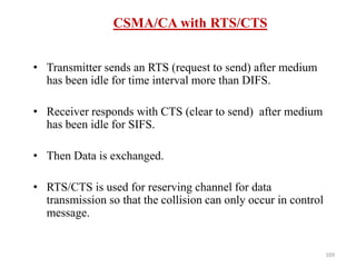
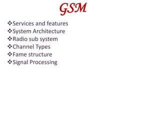
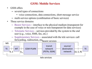
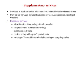
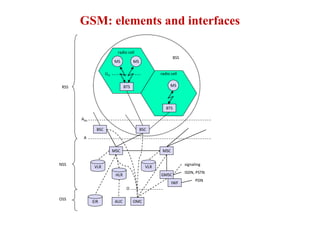
![ Common Air Interface (CAI)
Forward Channel
Reverse Channel
Standard that defines Communication
between a Base Station and Mobile
Specifies Four Channels [Voice
Channels and Control / Setup
Channels]
FVC: Forward Voice Channel
RVC: Reverse Voice Channel
FCC: Forward Control Channel
RCC: Reverse Control Channel](https://image.slidesharecdn.com/mobilecellularcommunication-230123165246-e8599357/85/Mobile-cellular-Communication-ppt-26-320.jpg)
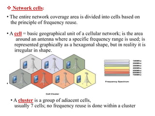
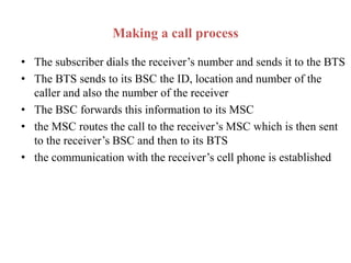
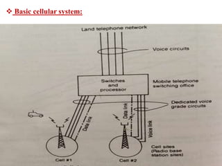
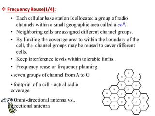
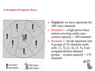
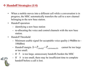
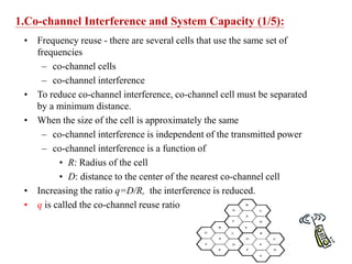
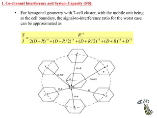
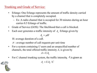
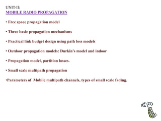
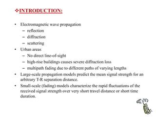
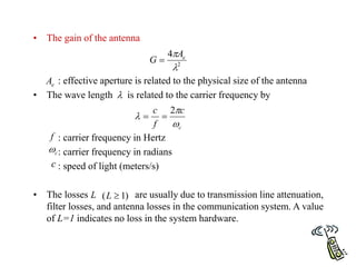
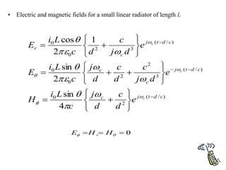
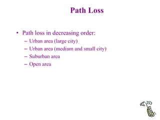
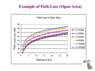
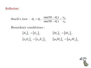
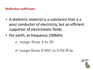
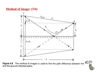
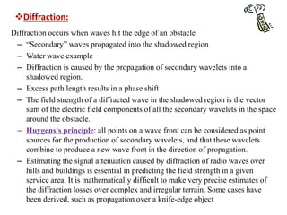
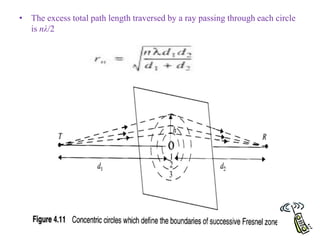
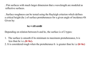
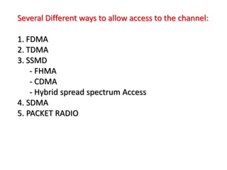
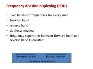
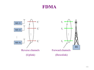
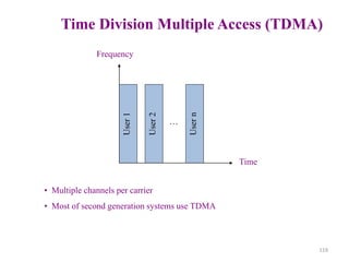
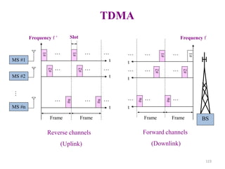
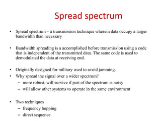
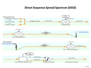
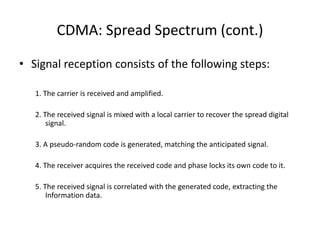
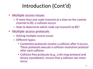
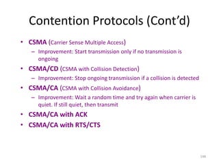
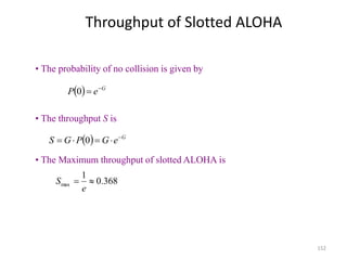
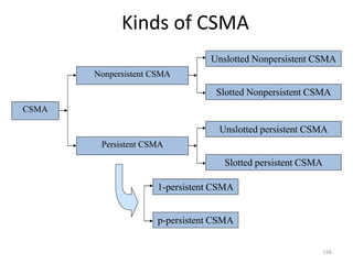
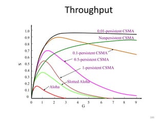
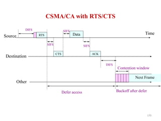
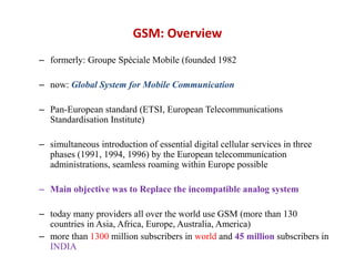
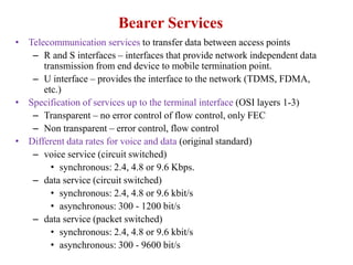
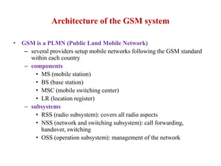
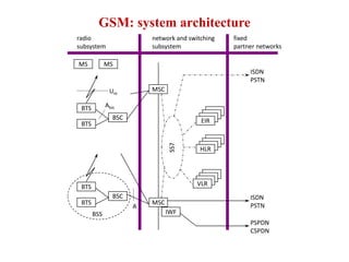
![Several Types of Mobile Radio Systems:
Garage Door Controller [<100 MHz]
Remote Controllers [TV/VCR/DISH][Infra-Red: 1-100 THz]
Cordless Telephone [<100 MHz]
Hand-Held Radio [Walki-Talki] [VHF-UHF:40-480 MHz]
Pagers/Beepers [< 1 GHz]
Cellular Mobile Telephone[<2 GHz]
Classification:
Simplex System: Communication is possible in only one direction :
Garage Door Controller, Remote Controllers [TV/VCR/DISH]
Pagers/Beepers
Semi-Duplex System: Communication is possible in two directions
but one talks and other listens at any time[Push to Talk System]:
Walki-Talki
Duplex System: Communication is possible in both directions at
any time: Cellular Telephone [FDD or TDD]](https://image.slidesharecdn.com/mobilecellularcommunication-230123165246-e8599357/85/Mobile-cellular-Communication-ppt-27-320.jpg)
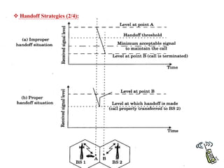
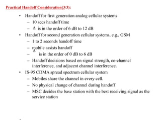
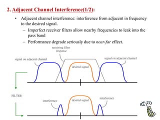
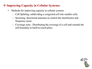
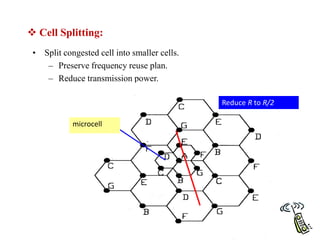
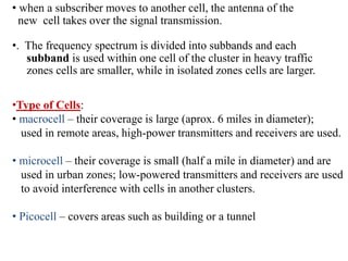
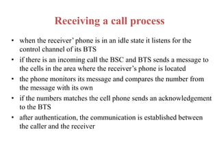
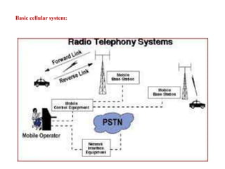
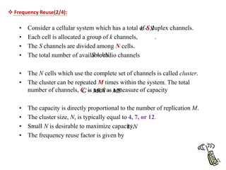
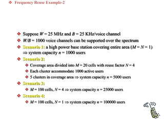
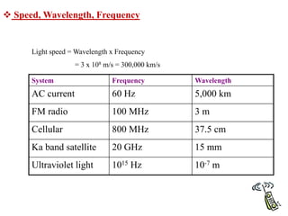
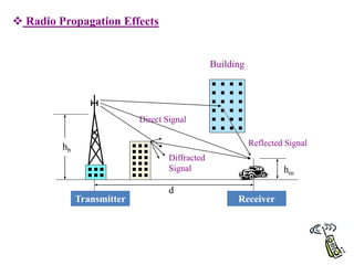
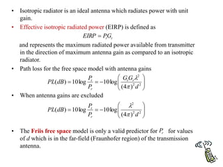
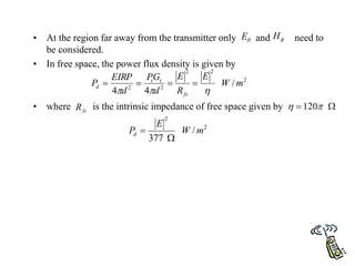
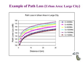
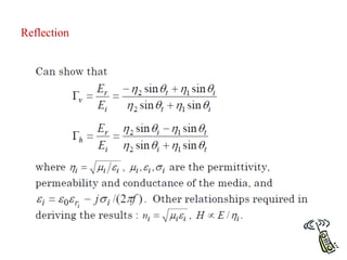
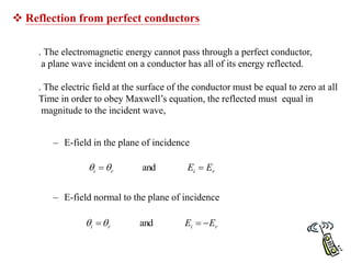
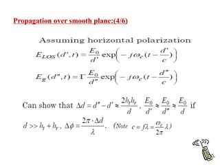
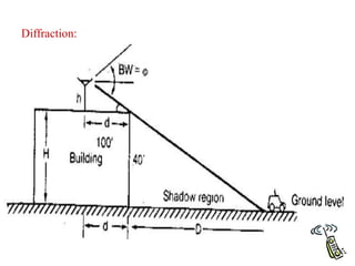
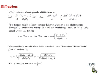
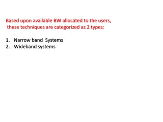
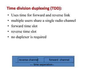
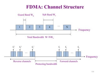
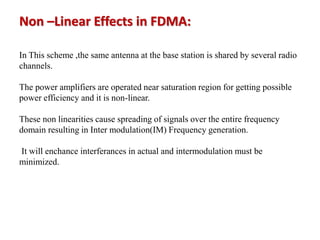
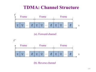
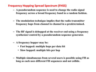
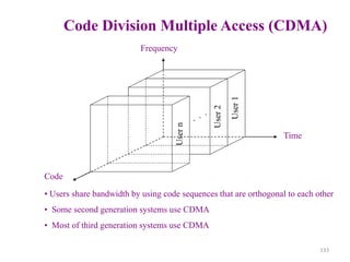
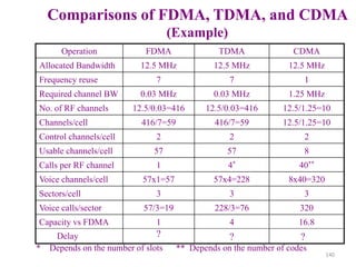
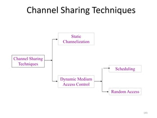
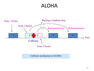
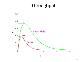
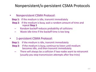
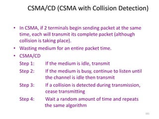
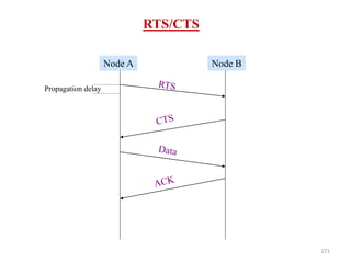
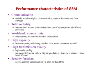
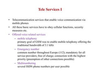
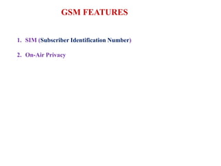
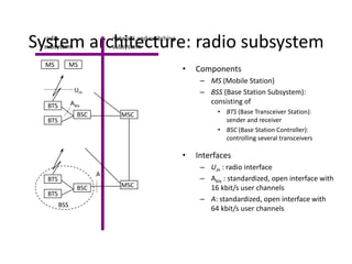
![• Transmission power reduction from to
• Examining the receiving power at the new and old cell boundary
• If we take n = 4 and set the received power equal to each other
• The transmit power must be reduced by 12 dB in order to fill in the
original coverage area.
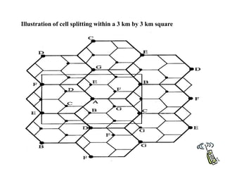
• Problem: if only part of the cells are splited
– Different cell sizes will exist simultaneously
• Handoff issues - high speed and low speed traffic can be
simultaneously accommodated
1
t
P 2
t
P
n
t
r R
P
P
1
]
boundary
cell
old
at
[
n
t
r R
P
P
)
2
/
(
]
boundary
cell
new
at
[ 2
16
1
2
t
t
P
P ](https://image.slidesharecdn.com/mobilecellularcommunication-230123165246-e8599357/85/Mobile-cellular-Communication-ppt-50-320.jpg)

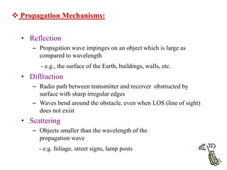
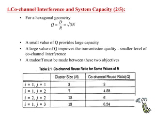
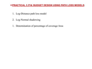
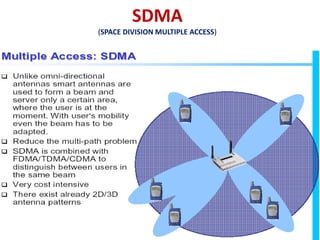
![RADAR CROSS SECTION MODEL:
• In Radio Channels where large, distant objects include scattering; knowledge of
the physical location of those objects can be used in order to accurately predict
scattered signal strength.
• RCS(Radar cross section): The RADAR cross section of a scattering object is
defined as the ratio of the power density of the signal scattered in the direction
of the receiver to the power density of the radio wave incident upon the
scattering object. It has units of square meters.
• For an URBAN mobile radio system, Models based on the bistatic radar equation are
Used to compute the received power due to SCATTERING in the far field.
Pr(dBm)=Pt(dBm)+Gt(dBi)+20 log (ʎ)+RCS[dBm2 ]-30log(4p)-20log dt-20log dr](https://image.slidesharecdn.com/mobilecellularcommunication-230123165246-e8599357/85/Mobile-cellular-Communication-ppt-101-320.jpg)


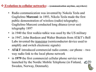
The document provides a comprehensive overview of the history and evolution of radio communication, highlighting key advancements from Nikola Tesla's and Guglielmo Marconi's early demonstrations to the development of mobile cellular networks. It explains the generational advancements in cellular technology (1G to 4G), the concept of frequency reuse, and the essential components and processes involved in mobile communications, such as call setup, handoffs, and channel assignment strategies. Additionally, it discusses various types of cells and interference management within cellular systems.


